Bayesian calibration of the mixing length parameter α_ML and of the helium-to-metal enrichment ratio ΔY/ΔZ with open clusters: the Hyades test-bed Free

ABSTRACT

1 INTRODUCTION

Theoretical stellar models are essential tools to infer the properties and characteristics of single or multiple stars in clusters/associations. Being theoretical computations, the accuracy of the models depends on the treatment of physical processes active in stars, which in turn strongly depends on the adopted input physics (e.g. equation of state, opacities, nuclear reaction rates, and outer boundary conditions, Tognelli, Prada Moroni & Degl’Innocenti 2011; Valle et al. 2013; Stancliffe et al. 2015). A crucial point in stellar modelling is the efficiency of convection in external superadiabatic regions. Despite the attempts to find a consistent description of the motion of matter in convective regions in stars using detailed hydrodynamical simulations, at the present it is not possible to follow the entire evolution of a star. Due to their complexity and long computational time, such simulations can be applied only to limited portions of a star, generally to boxes that cover a region of about 10⁶ m in the atmosphere (about 1–10 percent of the atmosphere, depending on effective temperature and surface gravity), then considered as representative of the whole atmospheric region. Moreover, such simulations have been obtained only for few selected evolutionary models (i.e. at selected stellar ages/evolutionary stages). To overcome these problems, simplified treatments of convection are adopted in stellar computations. The most used is the mixing length theory (Böhm-Vitense 1958), where the heat transport occurs in a region with a scale length ℓ proportional to the local pressure scale H_P, namely ℓ = α_MLH_P. The free parameter α_ML is the mixing length parameter, which has to be calibrated to reproduce real data. A method to estimate α_ML consists in reproducing the radius/colour index/effective temperatures of stars with a superadiabatic convective envelope. To do this, it is convenient to select stars in the mass range [0.6, 1.0] M_⊙, which corresponds to models strongly affected by a variation of α_ML.

Besides the input physics, stellar models are severely affected by the adopted chemical composition, especially the content of helium Y and the total metallicity Z (see e.g. Castellani, degl’Innocenti & Marconi 1999; Valcarce, Catelan & Sweigart 2012). Unfortunately, helium cannot be observed in the spectra of cold low-mass stars, but only in stars hotter than about 20 000 K, while the metallicity can be obtained – at least in principle – measuring the equivalent width of several metals absorption lines in stellar spectra.

The value of ΔY/ΔZ has been largely investigated in the past years. One of the possible method of constraining its value consists in comparing isochrones and stellar models in the HR diagram. Pioneering works involving the comparison between models and data of low-mass stars in the HR diagram was conducted by Faulkner (1967) and Perrin et al. (1977), who found respectively ΔY/ΔZ = 3.5 and 5. Pagel & Portinari (1998) used low-mass stars in the Hipparcos catalogue to obtain ΔY/ΔZ = 3 ± 2. Jimenez et al. (2003) re-analysed a sample of K dwarfs in the Hipparcos catalogue and they derive ΔY/ΔZ = 2.1 ± 0.4. A similar result was found by Casagrande et al. (2007) who obtained ΔY/ΔZ = 2.1 ± 0.9. Gennaro et al. (2010) performed a similar investigation on Hipparcos stars finding a much larger value ΔY/ΔZ = 5.3 ± 1.4. Moreover, they showed that the adopted age for the sample of stars deeply affects the results, leading to a systematic uncertainty on ΔY/ΔZ of about 2.

Another method to derive ΔY/ΔZ involves the construction of a standard solar model, where the present luminosity, radius, and surface (Z/X)_⊙ of the Sun has to be reproduced. This method gives a calibration of the α_ML parameter, and of the initial Y_ini,⊙ and Z_ini,⊙, from which ΔY/ΔZ for the Sun can be obtained. Such a value strongly depends on the input physics adopted to compute the solar model, and also on the observed (Z/X)_⊙. In particular, this last quantity has been largely revised in the last decades, changing more than 40 percent (see e.g. Grevesse & Noels 1993; Grevesse & Sauval 1998; Asplund, Grevesse & Sauval 2005; Asplund et al. 2009; Caffau et al. 2011). The consequence of such uncertainty on both (Z/X)_⊙ and the adopted input physics in solar models leads to values of ΔY/ΔZ that can vary between about 0.4 and 1.3 (see e.g Gennaro et al. 2010; Serenelli 2010; Tognelli et al. 2011; Valcarce et al. 2012).

There are other methods of determining ΔY/ΔZ, such as considering more evolved stars (horizontal branch and red giant stars, see Renzini 1994; Valcarce et al. 2016): in this case, values of ΔY/ΔZ between 2 and 3 are obtained. Another possibility is to constrain ΔY/ΔZ using galactic and extragalactic H ii regions (Peimbert & Torres-Peimbert 1974, 1976; Pagel et al. 1992; Peimbert, Peimbert & Ruiz 2000; Fukugita & Kawasaki 2006; Peimbert 2008; Méndez-Delgado et al. 2020) or planetary nebula (D’Odorico, Peimbert & Sabbadin 1976; Peimbert & Serrano 1980; Maciel 2001). These methods yield values of ΔY/ΔZ between 1 and 6 (see e.g. section 9 in Gennaro et al. 2010, for a detailed discussion).

The Hyades cluster is an ideal cluster to tightly constrain ΔY/ΔZ, because it is very close and it is not affected by extinction/reddening effects. Perryman et al. (1998) obtained a clean Hyades sequence using the early release of the Hipparcos parallaxes and used a sample of 40 main-sequence (MS) stars to constrain the cluster helium content. They found a helium abundance Y = 0.26 ± 0.02, where the central values was slightly smaller than their solar reference value. However, the large uncertainty they estimated (mainly due to the large photometric and distance uncertainty) did not rule out the possibility of having a larger helium content, as expected for such a metal-rich cluster. Lebreton, Fernandes & Lejeune (2001) analysed a double-lined eclipsing binary system in the Hyades (vB22, Peterson & Solensky 1988), which consist of a primary component with M₁ = 1.0591 ± 0.0062 M_⊙, and a secondary of about M₂ = 0.7605 ± 0.0062 M_⊙ (Torres & Ribas 2002): they found that only stellar models with subsolar helium content, namely Y = 0.255 ± 0.009 (Y_ini,⊙ = 0.2674), were compatible with the data. The authors concluded that this is the helium abundance in the Hyades cluster; however, the isochrone with subsolar helium content obtained from their fit starts to deviate from the observed Hyades MS at |$M_V \gtrsim 4$|–4.5 mag, as the clearly stated. A similar analysis was conducted by Pinsonneault et al. (2003): they derived a helium content for the vB22 binary system similar to their solar value. In the same years, Castellani et al. (2002) using the improved parallaxes provided by Madsen, Dravins & Lindegren (2002) obtained a very good fit of the Hyades sequence down to M_V ∼ 5.5 mag, where the models, and in particular the synthetic photometry used to convert the luminosity into magnitudes, suffer some problems. They found that models with a supersolar helium content (Y = 0.278), obtained using ΔY/ΔZ = 2 (Castellani et al. 1999), well matched the observed sequence. Casagrande et al. (2007) re-derived the helium content in the vB22 binary system confirming a slightly subsolar value. More recently, Gennaro et al. (2010) used faint stars in the Hyades cluster (M_V ≥ 5.2 mag) to infer the helium content of the cluster: from the analysis they obtained ΔY/ΔZ = 4.75 ± 0.35, which leads to supersolar helium content.

The aim of this paper is to apply a statistical method to analyse theoretically if it is possible to precisely calibrate stellar models on a portion of MS stars extracted from a cluster to derive the best value of ΔY/ΔZ and α_ML. To do this, we generated a set of synthetic stars to test the capability of the method to simultaneously recover the parameters used to generate the mock data set (i.e. [Fe/H], ΔY/ΔZ, and α_ML), and to identify possible systematic uncertainty sources. Then, we applied our method to the real data of MS stars in the Hyades cluster. This cluster is a good candidate for the present analysis because it is very close (about 47 pc), thus with a negligible reddening (E(B − V)|${\lesssim}0.001$| mag) and a very good precision on parallax and photometry. Moreover, it is old enough (500–700 Myr) that the location in the colour–magnitude diagram (CMD) of MS stars is insensitive to the age. All these characteristics helps in reducing the possible systematic uncertainties coming from unknown reddening, errors in distance, and age estimation.

The paper is structured as it follows. In Section 2, we describe the mock and real data sets and in Section 3, we describe the Bayesian code used for the analysis. The grid of models employed for the recovery is described in Section 4. In Section 5, we discuss the effects on the models of varying [Fe/H], ΔY/ΔZ, and α_ML. In Section 6, we present the results of the recovery procedure applied to the mock data sets. In Section 7, the same procedure is applied to the real Hyades data set. The conclusions and the results are then presented in Section 8.

2 THE SYNTHETIC AND HYADES DATA SAMPLE

With the aim to apply our method to Hyades cluster, we first tested it on a mock data set of synthetic MS stars, to evidence the possible biases and the minimal uncertainties of the procedure. To generate the synthetic stellar sample as close as possible to the real Hyades stars, we took as reference stars the Gaia DR2 Hyades data (Gaia Collaboration et al. 2016, 2018b), corrected for the distance modulus obtained from the parallaxes given by Gaia Collaboration et al. (2018a). We selected for our analysis the (G − Rp, B_P) plane, due to the very small uncertainties in these photometric bands (mean errors in magnitudes of about 0.002 mag, in the selected magnitude range, Gaia Collaboration et al. 2018b). We mention that Gaia DR2 data still suffers some systematics in both photometry and parallax zero-point definition (depending on the magnitude), estimated to be in the worst cases of about 0.01 mag in photometry (Evans et al. 2018) and of about 0.03–0.05 mas in parallax (Lindegren et al. 2018; Zinn et al. 2019; Schönrich, McMillan & Eyer 2019). We investigated the possible effect of such errors in the synthetic data sets, as discussed below.

The first step was to select the MS portion to be used in the procedure, according to the following requirements: (1) independence of the age, (2) good agreement between theoretical models and data, and (3) dependence on helium-to-metal enrichment ratio, ΔY/ΔZ. An additional requirement is that the selected region is unaffected by not well-constrained parameters used in stellar models, such as the core overshooting parameter (see e.g. Saslaw & Schwarzschild 1965; Shaviv & Salpeter 1973).

Fig. 1 shows a qualitative comparison between the Gaia Hyades sequence and our partial isochrones in the selected mass range [0.4, 1.5] M_⊙ that satisfies the three conditions discussed above. Notice in particular that the location of the MS in this mass interval is almost independent of the age,¹ within the current uncertainty, as proven by the superposition of the three isochrones with ages 300, 500, and 700 Myr. Thus, to avoid age dependence we have adopted a cut-off magnitude of B_P = 3.5 mag (about 1.4 M_⊙).

Figure 1.

Hyades sequence in the Gaia CMD, data from Gaia Collaboration et al. (2018a), compared to our partial isochrones with [Fe/H] = +0.16 (ΔY/ΔZ = 2 and α_ML = 2) and three different ages, namely 300 (dashed line), 500 (solid line), and 700 Myr (dashed–dotted line): the isochrones at different ages overlap almost perfectly along the whole sequence. The part of the sequence selected for the analysis is shown as blue-filled triangles.

Open in new tabDownload slide

From the same figure, it is also evident that the agreement between data and models is very good for B_P magnitudes below 6–7 mag, while for fainter stars the observed sequence significantly deviates from the theoretical one (reaching a maximum difference in colours of about 0.06 mag). To address the problem of the origin of this discrepancy, which has been observed by different authors using several theoretical models and which is already discussed in the literature (see e.g. Gagné, Faherty & Mamajek 2018) is out of the purposes of this paper. It is common opinion that part of the disagreement is caused by the atmosphere models used to obtain the synthetic spectra, which still have problems in correctly predicting the flux in the optical/blue part of the spectra (e.g. Kučinskas et al. 2005; Casagrande & VandenBerg 2014). Indeed, such a wrong behaviour, that is the bend of theoretical models towards bluer colours, does not occur when infrared colours – such as 2MASS magnitudes – are used, down to 0.1–0.2 M_⊙ (Kopytova et al. 2016). However, the observations in infrared colours do not achieve the high photometric precision required for our analysis. To use the Gaia DR2 data we were forced to limit the analysis to a smaller portion of the observed MS. In particular, we restricted to B_P ≤ 6.5 mag (about 0.8 M_⊙). In this magnitude range, we also removed from the real cluster 3 stars that are obviously out of the MS sequence (suspected unresolved binaries). Thus, we have a sample of observed 49 stars and we can built the synthetic data set with the same number of stars.

Having selected the portion of MS to be used, we tested the capability of the statistical method to constrain the parameters we are interested in ([Fe/H], ΔY/ΔZ, and α_ML) from the (G − Rp, B_P) plane taking into account the uncertainties on the observable quantities, using different mock data sets of artificial stars with characteristics similar to those of the Hyades. In particular, we explored the effects on the result of different choices on (1) the photometry/distance errors, (2) number of stars, and (3) portion of MS used in the recovery. We define the sets of synthetic data as described in the following:

• TYPE_0: the set used only to test the recovery algorithm and to evaluate possible systematic biases. It consists of a set of 50 synthetic stars with an unrealistic small error in magnitudes, that is, 0.00005 mag, in the selected B_P range [3.5, 6.5] mag, which corresponds to populate the isochrone in the mass range [0.83, 1.35] M_⊙. The synthetic data set is calculated for [Fe/H] = +0.16, ΔY/ΔZ = 2, α_ML = 2, and an age of 500 Myr. This set is designed to evidence biases due to the recovery procedure, since the simulated observational errors are extremely small.²

• TYPE_1: we adopted an uncertainty of 0.002 mag on the colour index (G − R_P) and 0.011 mag on the B_P absolute magnitude. The uncertainty on the colour index is designed to mimic the mean value of the errors of the Gaia colours for the Hyades in the adopted B_P magnitude range. The error on the absolute magnitude B_P corresponds to the uncertainty on the magnitude quoted by the Gaia Collaboration (0.001 mag) plus an uncertainty of about 0.01 mag on the distance modulus. This last quantity was evaluated using the estimated parallax uncertainty, π = 21.15 ± 0.04 mas (Gaia Collaboration et al. 2018a) and a systematic parallax error of 0.1 mas (Gaia Collaboration et al. 2018b). We populated a theoretical isochrone in the mass range [0.83, 1.35] M_⊙, which corresponds to an absolute magnitude range B_P ∈ [3.5, 6.5] mag. We simulated N_s = 50 stars, a number similar to that found for the real Hyades cluster in the selected magnitude range. This case is designed to be as close as possible to the real Hyades data.

• TYPE_2: we used the same errors on photometry as in TYPE_1, but we reduced the systematic error on the parallaxes to 0.01 mas. Thus, the adopted uncertainty on B_P mag is 0.005 mag.

• TYPE_3: as in TYPE_1, but for a larger sample of stars that extends down to B_P = 10 mag. We adopted the following parameters, N_s = 100 in the magnitude range B_P ∈[3.5, 10] mag, which corresponds to a mass range [0.5, 1.35] M_⊙.

3 RECOVERY PROCEDURE

4 THE GRID OF MODELS

We constructed a grid of stellar models using the pisa stellar evolutionary code (Degl’Innocenti et al. 2008; Dell’Omodarme et al. 2012) in the same configuration described in previous papers (Tognelli, Prada Moroni & Degl’Innocenti 2015, 2018). We briefly mention the main input parameters/physics that are relevant for the present analysis, which are the convection efficiency in superadiabatic regions, the outer boundary conditions (atmospheric models) and the solar mixture (metal relative abundance in the Sun). For the last quantity, we adopted the Asplund et al. (2009) metal distribution. Concerning the superadiabatic convection efficiency, we used the mixing length theory (Böhm-Vitense 1958) which is characterized by the dependence on a free parameter (the mixing length scale), α_ML. Such a quantity is a free parameter that has to be calibrated. A common way of calibrating α_ML consists in constructing a standard solar model, which is a 1 M_⊙ model that at the age of the Sun has to reproduce simultaneously the solar radius, luminosity, and (Z/X)_⊙ within a given tolerance. These three quantities depends on the initial values of helium Y_ini,⊙, metallicity Z_ini,⊙ and α_ML: from the solar calibration, we obtained α_ML⊙ = 2.0016, Y_ini,⊙ = 0.2624, and Z_ini,⊙ = 0.01524. Another key ingredient for the computation of models with a convective envelope (in our case for MS stars with |$M\lesssim 1$| M_⊙) is the adopted outer boundary conditions (i.e. atmospheric structure) needed to specify the pressure and temperature at the bottom of the atmosphere to close the system of differential equations that describes the stellar structure. We adopted the Allard, Homeier & Freytag (2011) pre-computed models, obtained using input physics very similar to that we used for the computation of the interior structure of the star. The consistency between atmospheric and interior structure, in particular the treatment of convection, is a crucial point to avoid the inclusion of uncontrollable systematic effects. We emphasize that the value of α_ML we obtained with the solar calibration is basically the same used for the computation of the atmospheric structure (i.e. α_ML,atm = 2.0), which results in a very similar convection treatment in the interior and in the atmosphere, thus giving to the models a high level of internal consistency.

The required mass range for the model grid to be compared with the Hyades sequence is |$0.8\lesssim M/$|M_⊙|${\lesssim}1.4$|⁠. However for some of the test cases we needed a wider mass range. So, we computed 18 stellar models in the mass range M ∈[0.4, 1.5] M_⊙ with a variable spacing (0.05 M_⊙ for M ≤ 1.0 M_⊙ and 0.1 M_⊙ for larger masses), each for 11 [Fe/H] values in the range [+0.08, +0.28] dex with a spacing of 0.02 dex, to covers the range of recent spectroscopic determinations with the related errors. For each value of [Fe/H] we adopted 11 values of ΔY/ΔZ in the range [1, 3] with a spacing of 0.2. Moreover, each model set specified by a given value of mass, [Fe/H], and ΔY/ΔZ has been calculated for five different values of α_ML in the range [1.8, 2.2] with a spacing of 0.1. The selected α_ML values are chosen to cover a symmetric interval about our solar calibrated mixing length parameter (namely α_ML = 2). In total, we computed 605 sets of stellar models.

The parameters estimation algorithm relies on the set of pre-computed isochrones (to reduce the computational time of the recovery procedure), and no interpolation is performed on the fly. Therefore, a dense grid is needed to achieve a high accuracy in the results and to avoid noisy behaviours (see also Bazot et al. 2016). To do this, the displacement of a model at a fixed mass in the CMD due to the variation of each parameter in the grid (i.e. [Fe/H], ΔY/ΔZ, and α_ML) must be smaller than the observational uncertainty. To this regard, the average smallest error is about 0.002 mag, and it comes from the G − Rp, colour index. We verified that to achieve a good likelihood in the recovery (smooth and without spurious peaks) we need a variation of about one-half/one-third of such an uncertainty. The grid spacing (in each parameter) has been consequently tuned to satisfy this requirement, by interpolating the models on a finer grid before running the recovery procedure: we adopted a spacing of 0.005 dex in [Fe/H], 0.05 in ΔY/ΔZ, and 0.02 in α_ML, for a total of |$35\, 301$| sets of stellar models. We checked (extracting some cases from the grid) that the interpolation produces models in a very good agreement with those obtained by a direct computation by means the stellar evolutionary code (negligible differences).

Having constructed the grid of models, we generated the isochrones in range of age [300, 700] Myr and we converted them to Gaia magnitudes using the bolometric corrections obtained from the MARCS2008 synthetic spectra (hereinafter M08, Gustafsson et al. 2008), and the magnitude zero points given in Evans et al. (2018).

5 EFFECT OF CHANGING α_ML, [FE/H], AND ΔY/ΔZ

Before starting the analysis, it is useful to remind the effect of [Fe/H], α_ML, and ΔY/ΔZ on theoretical isochrones. Fig. 2 shows the effect of varying separately α_ML, [Fe/H], and ΔY/ΔZ within the selected range on a 500 Myr isochrone both in the HR and the CMD.

Figure 2.

Change of the position of a 500 Myr isochrone in the HR (left-hand column) and Gaia CMD (right-hand column) caused by a variation of the mixing length parameter (top panels), [Fe/H] value (middle panels), and ΔY/ΔZ (bottom panels).

Open in new tabDownload slide

Concerning the mixing length (top panels), it is well known that the effect strongly depends on the stellar mass. The T_eff and R of stars with |$M \lesssim 0.4$|–0.5 M_⊙ (i.e. |$B_P \gtrsim 10$|⁠) in MS are independent of the the value of α_ML because the structure is dense enough to have an almost adiabatic temperature gradient even in external regions of the star. On the other hand, increasing the stellar mass, the star gets progressively more and more superadiabatic in the external convective layers, showing a progressively stronger dependence on α_ML. However, the convective envelope gets thinner and thinner as the mass increases, consequently the sensitivity on α_ML first increases and then decreases and eventually vanishes for |$M\gtrsim$|1.2–1.4 M_⊙ (⁠|$B_P \lesssim 3.5$| mag). This means that the impact of α_ML on the CMD location of an isochrone is not rigid but depends on the stellar mass (or equivalently on the magnitude): at fixed B_P magnitude a variation of α_ML of ±0.25 results in a colour change of about 0.01 mag for B_P ∈ [3.7,  5] mag which progressively (almost linearly) decreases to about 0.005 mag at B_P ≈ 6–6.5 mag.

Middle panels of Fig. 2 show the effect of varying the initial value of [Fe/H]. The a variation of [Fe/H] results in a change of both Y and Z, although the net variation of Z is much larger than the variation of Y. As an example, moving from [Fe/H] = +0.16 to +0.22 results in a change of about 14 percent in Z and about 2 percent in Y. The effect on the models of a variation of [Fe/H] in the range [+0.10, +0.22] is smaller than that due to the change of α_ML, and it is almost the same for all the models along the isochrone. Only low-mass stars tail (log L/L_⊙|${\lesssim}-1.2$| or |$Bp \gtrsim 9~$|mag which corresponds to |$M\lesssim 0.6$| M_⊙) show a slightly different dependence on [Fe/H]. An increase of [Fe/H] of +0.06 dex produces a rigid shift to the right-hand part of the diagram (cooler models), at fixed B_P magnitude, of about 0.005–0.006 mag in the colour index (in the selected magnitude interval B_P ∈ [3,  7] mag). Low-mass star tail (⁠|$M \lesssim 0.6$| M_⊙) of the isochrone exhibits a slightly larger dependence on [Fe/H] than the region populated by more massive stars.

Bottom panels of Fig. 2 show the effect of a variation of ΔY/ΔZ. A variation of ΔY/ΔZ at fixed [Fe/H] affects mainly the helium content. Similarly to [Fe/H], the variation of the initial helium content produces an almost rigid shift of the isochrone in the HR/CMD. In particular, an increase of ΔY/ΔZ of 1 moves the models towards the left-hand part of the plane (hotter models) of about 0.005–0.007 mag in the colour index at a fixed B_P magnitude.

An increase of ΔY/ΔZ has an effect opposite to that caused by an increase of [Fe/H]. Thus, depending on the adopted ΔY/ΔZ and [Fe/H] it is possible that the two effects balance each other. An example is shown in Fig. 3, where we plotted a 500 Myr isochrone with the reference chemical composition ([Fe/H] = +0.16 and ΔY/ΔZ = 2) together with two other 500 Myr isochrones, one with [Fe/H] = +0.10 and ΔY/ΔZ = 1 and the other with [Fe/H] = +0.22 and ΔY/ΔZ = 3. The three models are very close both in the HR and Gaia CMD. There is only a slight difference in HR diagram in the middle part of the isochrone, while for the CMD only at the faint tail of the isochrone (out of the region selected in the present analysis) very small differences are visible. This figure clearly shows that, as well known in the literature, it exists a certain level of degeneracy between [Fe/H] and ΔY/ΔZ in a large part of the MS; in particular a variation of ±0.06 dex in [Fe/H] can be almost entirely balanced by a variation (in the same direction) of ±1 in ΔY/ΔZ (see e.g. Castellani et al. 2002) both in the CMD and the HR diagram. However, this is not completely true for the low-mass tail of the isochrone (⁠|$B_P \gtrsim 9$|–10 mag, thus for |$M\lesssim 0.6$| M_⊙): the presence of such a low-mass tail could mitigate the ΔY/ΔZ–[Fe/H] degeneracy.

Figure 3.

Effect on the position of a 500 Myr isochrone in the HR and Gaia CMD of the simultaneous variation of ΔY/ΔZ and [Fe/H] with respect to the reference chemical composition. The reference isochrone (ΔY/ΔZ = 2 and [Fe/H] = +0.16, grey line) is compared to isochrones with ΔY/ΔZ = 1 and [Fe/H] = +0.10 (blue dashed line) and ΔY/ΔZ = 3 and [Fe/H] = +0.22 (red dashed line).

Open in new tabDownload slide

This qualitative analysis suggests that, in this work, due to the restrictions on the MS portion suitable for the analysis, it might be difficult to reach an high precision in the simultaneous derivation of ΔY/ΔZ and [Fe/H] using MS stars. This problem could be overcame if a reliable spectroscopic estimate of [Fe/H] is available.³ In this case, the adoption of a proper prior on [Fe/H], could be used to constrains the interval of reasonable [Fe/H] values and consequently to better constrain the ΔY/ΔZ value.

6 TESTING THE PERFORMANCE OF THE RECOVERY PROCEDURE ON SYNTHETIC DATA SETS

Before performing an analysis on real Hyades data, it is mandatory to test the capability of the method on a synthetic data set to highlight the bias and the uncertainties related to the recovery of the selected parameters. Thus, the first step is to prove the capability of the algorithm to recover the true parameters, that is, those used to generate the synthetic data set of artificial stars sampled from the same grid of theoretical models used in the recovery itself. More in detail, the mock data have been obtained by taking one of the isochrone available in the grid (with a given set of [Fe/H], ΔY/ΔZ, and α_ML), populating it with a given initial mass function (not important for the present analysis), and then by applying a Gaussian perturbation (error) on the magnitudes of each synthetic star to simulate the observational uncertainty.

It is worth noticing that such a preliminary test corresponds to the best configuration, because the physics adopted in the models of the recovery grid is the same used to construct the data set. In the real world one expects some differences between the physics of observations and of the models which can lead to additional biases and uncertainties.

6.1 TYPE_0 data set: ideal data set

The first test was performed on a mock data set with negligible observational errors (TYPE_0, 0.00005 mag on the magnitude), which means that the simulated MS stars are not scattered with respect to their original position on the MS. This step is necessary to evaluate the presence of a possible systematic hidden inside the procedure. We generated 50 stars in the B_P range [3.5, 6.5] mag at 500 Myr adopting as reference values [Fe/H] = +0.16, ΔY/ΔZ = 2, and α_ML = 2.

We applied the recovery procedure to the artificial stars, for two different choices about the adopted prior for the [Fe/H] value: (1) no prior, all the [Fe/H] values are equally probable, and (2) a Gaussian distributed [Fe/H] centred on the value adopted for the synthetic data set. Independently of the adopted prior on [Fe/H], in all the cases, the most probable values of [Fe/H], ΔY/ΔZ, and α_ML obtained from the recovery procedure are exactly the same used to generate the data sample. The CI (credible interval of each recovered parameter) is much smaller than the step on the grid of models. Thus, we can conclude that, on a set of synthetic data with a negligible observational errors, the method does not show any systematic or bias.⁴

6.2 TYPE_1 data set: Hyades-like data set

After the validation of the method, we applied the analysis to the TYPE_1 data set, which was generated to obtain a data set as close as possible to the Hyades. We adopted the same chemical composition and α_ML of the TYPE_0 data set. We selected the interval of magnitude/colours, errors, and number of stars, as described in Section 2: we simulated 50 stars in the B_P range [3.5, 6.5] mag, with a Gaussian distributed error on the G − R_P colour of 0.002 and 0.012 mag on the B_P magnitude. As said before, the relatively large error on B_P – if compared to that on the colour – comes from the systematic parallax uncertainty of 0.1 mas (i.e. an error in the distance modulus of about 0.01 mag).

We ran the recovery procedure to simultaneously derive the most probable values of ΔY/ΔZ, α_ML, and [Fe/H]. The top panels of Fig. 4 show the marginalized likelihood for [Fe/H], ΔY/ΔZ, and α_ML for a flat prior on [Fe/H]. [Fe/H] is badly recovered from the analysis. The most probable value (peak of the distribution) is at about [Fe/H] = +0.09, whereas the true one is +0.16, and the derived CI on [Fe/H] is very broad, from about [Fe/H] = +0.08 to about +0.18. The shape of the likelihood shown in figure deserves a discussion. The peak at [Fe/H] = +0.09 dex, very close to the edge of the grid, shows that in this first test the value of [Fe/H] is badly recovered by the procedure. The mixing of [Fe/H], ML, and ΔY/ΔZ on the grid is so strong that the method fails in identifying the true value of [Fe/H] used to simulate the data in this mock data set.

Figure 4.

Posterior marginalized distributions for TYPE_1 data set, for [Fe/H] (left-hand panels), ΔY/ΔZ (middle panels), and α_ML (right-hand panels), for two choices of the prior on the metallicity, namely flat (top panels) and Gaussian with [Fe/H]_pr = +0.16 dex and σ_FeH = 0.02 dex (bottom panel).

Open in new tabDownload slide

Similarly to [Fe/H] also ΔY/ΔZ is badly recovered and, as shown in figure, the peak is at ΔY/ΔZ≈1.5, thus underestimating the value of about 0.5, with a large CI, ΔY/ΔZ = [1.2, 2.3]. The large CI in ΔY/ΔZ, comes essentially from the large CI in [Fe/H].

The distribution of the α_ML values looks better. Indeed, as showed in the previous sections, a change in α_ML affects the models along the isochrone in a differential way, thus producing a different slope of the isochrone in the plane used for the analysis. Moreover, for B_P ∈ [4,  6] mag, the isochrones are very sensitive to the adopted α_ML and even a small change in α_ML produces a relatively large effect on the models. This allows a better identification of the most probable value (i.e. the peak and the width of the marginalized likelihood). The recovered value is only 1.5 percent lower than the true one, and the corresponding CI is not very large, α_ML∈ [1.92,  2.06].

From the analysis we can conclude that, as expected, the unavailability of independent [Fe/H] determinations drastically complicates the problem of deriving ΔY/ΔZ and/or [Fe/H] values with this method even when synthetic data are used. More importantly, the derived values of [Fe/H] and ΔY/ΔZ are affected by a large bias. This result is expected and it is the consequence of the degeneracy between [Fe/H] and ΔY/ΔZ values, and of the weak dependence of the models on [Fe/H] and ΔY/ΔZ.

We tested whether the availability of an independent estimate of [Fe/H] might be used to improve the goodness of the recovery. To do this, we assumed a Gaussian prior on [Fe/H]. This prior was centred at [Fe/H]_pr = +0.16 dex (the value used to simulate the data), with a dispersion of σ_FeH = 0.02 dex. The results are shown in the bottom panel of Fig. 4. The posterior distribution of [Fe/H] – obtained from the analysis – is close to a Gaussian, and the most probable value of [Fe/H] (i.e. +0.158) and the dispersion (CI) [+0.017, −0.021] are very similar to those used in the prior. This result points out an important fact, which is that in presence of a prior distribution well peaked at a certain value of [Fe/H], the posterior distribution is strongly influenced by the prior. This is clear if one looks at the posterior distribution of [Fe/H] (also of ΔY/ΔZ) when no prior is adopted (top left panel of Fig. 4). The distribution is very broad and the inclusion of a Gaussian prior overcomes any information available from the original distribution. The recovered [Fe/H] value is basically defined by the prior.

Also the ΔY/ΔZ distribution looks better when the Gaussian prior on [Fe/H] is adopted. The distribution of ΔY/ΔZ shows a clear peak (at variance with the result for the flat-prior case). The most probable value of ΔY/ΔZ is 1.99 (basically equal to the true one), with a narrow CI (i.e. between 1.69 and 2.17). Concerning the mixing length parameter, the distribution of α_ML is almost independent of the prior on [Fe/H], and the most probable value of α_ML is equal to the simulated one with a very small CI, namely [1.97, 2.05]. Such a good accuracy on ΔY/ΔZ is a consequence of the prior effect on [Fe/H] distribution: indeed, given the degeneracy [Fe/H]–ΔY/ΔZ in isochrones, once [Fe/H] is derived with a good accuracy, also ΔY/ΔZ can be obtained with a relative high accuracy.

As a final comment, this first data set clearly shows that only the mixing length parameter can be recovered (independently) without any additional information (i.e. prior) from this set of data. The other quantities, [Fe/H] and ΔY/ΔZ are badly recovered if no prior on [Fe/H] is specified. On the other hand, the inclusion of a Gaussian prior allows to derive values for the [Fe/H] prior, ΔY/ΔZ close to that used to generate the data set. However, the values of the parameters and their CI might be affected by the adopted prior on [Fe/H], that is, [Fe/H]_pr and σ_FeH. The dependence of the results on the adopted [Fe/H] value in the prior must be taken into account when the method is applied to the real data, as we will discuss it in the next sections.

6.3 TYPE_2 data set: Hyades-like data set with artificially reduced systematic parallax errors

As a next step, we checked whether the results are affected or not by a realistic future reduction of the observational uncertainties, in particular we want to analyse the effect of a possible reduction of the uncertainty in the parallax. We recall that the assumed uncertainty on the B_P mag in the TYPE_1 set was dominated by the uncertainty in the distance, a systematic uncertainty of 0.1 mas. Such an uncertainty is expected to be reduced at the end of the Gaia mission, so it is worth to evaluate the impact of it on the derived parameters. To do this, we generated another sample of synthetic data, with the same characteristics of the TYPE_1 data set, but with a uncertainty on the B_P mag reduced by a factor of 2, that is, error(B_P) = 0.005 mag (TYPE_2). We applied the method to this data set and we found that the reduction of the distance uncertainty does not produce any appreciable effect on the recovered parameters or on the derived CI.

6.4 TYPE_3 data set: extended Hyades-like main-sequence data set

We performed another test in which we increased the extension of the observed sequence used to compare models and data, TYPE_3. In this case, we included faint stars in our sample, down to M ∼ 0.5 M_⊙, which corresponds to stars with B_P ∈ [3.5, 10] mag. Having increased the magnitude interval, we also increased the number of simulated stars to 100 (as in the real Hyades cluster for the same magnitude interval). The errors are the same used in TYPE_1 case (namely err(B_P) = 0.012 mag and err(G − R_P) = 0.002 mag).

The use of a more extended sequence leads to the best results, both with and without a Gaussian prior on the metallicity. The reason for such an improvement is double. On one hand, the inclusion of fainter stars (i.e. |$B_P\gtrsim 9.5$|–10 mag) partially removes the degeneracy [Fe/H]−ΔY/ΔZ, as we discussed in Section 5. Such stars are affected by the helium and [Fe/H] variation in a different way with respect to brighter ones. The same couple of [Fe/H] and ΔY/ΔZ that produces (almost) overlapping MS for brighter stars does not lead to the same overlap for fainter stars. This gives the possibility to obtain more precise results. On the other hand, having extended the sequence (i.e. the magnitude interval) we have more stars, which in our case is twice those in TYPE_1, thus reducing the statistical fluctuations.

Fig. 5 shows the result of the recovery for TYPE_3 data set for the two choices on the prior on the metallicity, namely flat (top panels) and Gaussian centred in [Fe/H]_pr = +0.16 dex with σ_FeH = 0.02 dex (bottom panels). The most interesting difference with respect to TYPE_1 data set is achieved when a flat prior on [Fe/H] is adopted. Even in this case, the most probable values of [Fe/H], ΔY/ΔZ, and α_ML are extremely close to the true ones, that is, those used to generate the synthetic data sample, and the corresponding CI obtained in the TYPE_3 flat prior case are very small if compared to those obtained in TYPE_1 flat prior test. It is also interesting to notice that the quality of the results is not improved if the Gaussian prior on the metallicity is adopted (bottom panels). This is due to the fact that the selected sequence is extended enough to clearly disentangle the effect of a variation of [Fe/H], ΔY/ΔZ, and α_ML. So, this data set would correspond to an ideal configuration to derive the parameters, in the sense that we would expect the results to be more precise than those obtained in the other cases. Unfortunately, as already discussed, the whole MS |$B_P \in [3.5,\, 10]$| mag, cannot be used for comparison with real data, due to the large current disagreement between predictions and observations for |$B_P \lesssim 6.5$|–7 mag.

Figure 5.

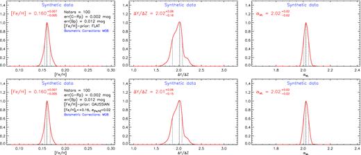
Posterior marginalized distributions as in Fig. 4, but for TYPE_3 data set.

Open in new tabDownload slide

6.5 Effect of a systematic error in [Fe/H]

In the previous section, we showed that the estimate of stellar parameters is affected by the functional form, flat or Gaussian, of the assumed prior on [Fe/H] even if the prior distribution if centred on the true value. It is thus natural to expect a stronger impact on the recovered parameters of the adopted prior on [Fe/H] whenever a systematic bias in its determination is present. When dealing with real stellar cluster rather than synthetic ones, it is common to have quite different spectroscopic estimates. This section is then devoted to analyse the effect of systematic bias in the adopted value of [Fe/H]_pr and σ_FeH on the estimate of stellar parameters. For what concerns real data, the value of [Fe/H] measured by several authors for the same cluster might vary more than the quoted uncertainties (because of the use of a sample of different stars, or a different analysis technique, or the adoption of different calibration for the [Fe/H] scale). If this is the case, it is not so straightforward to choose the best value of [Fe/H] to be used in the prior and its dispersion. Thus, one should be aware that [Fe/H]_pr and σ_FeH can alter the estimate of the parameters at some level that we want to quantify.

To do this, we run the recovery using a grid of [Fe/H]_pr, from +0.12 to +0.20 in step of +0.01, to cover a plausible range of [Fe/H]_pr. Since the prior also depends on the width of the distribution σ_FeH, we used for each value of [Fe/H]_pr three values, σ_FeH = 0.02, 0.03, and 0.05≡ {σ_FeH,j}. We used these values to construct a grid of Gaussian priors each with a couple ([Fe/H]_pr,j, σ_FeH,j). Then, we run the recovery over the TYPE_1 data set, and we obtain for each choice of the Gaussian prior ([Fe/H]_pr,j, σ_FeH,j) the most probable value of [Fe/H], ΔY/ΔZ, and α_ML with the corresponding CI. Fig. 6 shows the results of the recoveries, for a Gaussian prior with a width σ_FeH = 0.02 (first row), 0.03 (second row), and 0.05 (third row). Fig. 6 also shows the results obtained using different indicators for the most probable value and for the CI. In particular we used: (1) the mode (our reference) to define the most probable value and the 16th and 84th percentile for the CI, (2) the median for the most probable value and the 16th and 84th percentile for CI, and (3) the mean and the rmsd.

Figure 6.

Most probable value and corresponding CI for [Fe/H] (first column), ΔY/ΔZ (second column), and α_ML (third column) for TYPE_1 data set, as a function of [Fe/H]_pr and for three values of σ_FeH = 0.02, 0.03, and 0.05 dex (first, second, and third rows, respectively). The best value and the relative CI obtained using the median and the mean (see the text) are also shown.

Open in new tabDownload slide

For what concerns [Fe/H], the recovered values of [Fe/H] resembles the value used in the prior depending on the value of σ_FeH,j. If the range of [Fe/H] values allowed by the prior distribution is well peaked, that is, σ_FeH = 0.02, then the recovery is forced to use [Fe/H] values close to [Fe/H]_pr, and the derived [Fe/H] is very close to [Fe/H]_pr. If the width of the prior is larger (i.e. 0.03 or 0.05), the best value of [Fe/H] can be different from the prior value. From Fig. 6 (top panel), it is evident that by increasing σ_FeH the derived CI on [Fe/H] increases too: in general, the uncertainty on the derived [Fe/H] (i.e. the CI) is similar to σ_FeH. In any case, the derived [Fe/H] value is biased by the adoption of the prior.

The most probable value of ΔY/ΔZ is affected by ([Fe/H]_pr,j, σ_FeH,j). As a general comment, ΔY/ΔZ varies at maximum between 1.5 and 2.3, depending on [Fe/H]_pr(about 15–25 percent), so it includes the true value (ΔY/ΔZ = 2). As expected the CI of the recovered ΔY/ΔZ is affected by σ_FeH, but not as much as for [Fe/H]: the largest is σ_FeH and the broader is ΔY/ΔZ CI, namely about 0.3 (about 15 percent) at σ_FeH = 0.02 dex and 0.4–0.5 (about 20–25 percent) at σ_FeH = 0.05 dex. This results show that also ΔY/ΔZ is affected by a bias if a prior on [Fe/H] is adopted, a bias that can reach 0.3–0.5.

Concerning α_ML, as already noted, its value is less affected by the adopted prior on [Fe/H] and in all the cases, the recovered value is very close to the true one, and fully compatible with it within its CI. To be noted that α_ML varies at maximum of about 2–3 percent considering all the possible values of ([Fe/H]_pr,j, σ_FeH,j). So, this parameter is recovered with a very high precision and accuracy if compared to ΔY/ΔZ and [Fe/H].

In any case, we can firmly state that in this particular data set, the adoption of a prior on [Fe/H] necessarily introduces a not negligible bias in all the recovered parameters but α_ML.

Fig. 6 also shows that the three different indicators used to specify the most probable value and/or the CI generally agree, or, in any case, the difference among the results is smaller than the quoted CI. Noticeably, the CI obtained using the percentiles or the rmsd are essentially the same in all the cases.

The same analysis was repeated using the TYPE_3 data set, that is, the set with the MS extended down to B_P = 10 mag. The results are shown in Fig. 7. This case is very close to the ideal one. Almost independently of the adopted [Fe/H]_pr or σ_FeH, the recovered parameters are affected by a negligible bias, they are in all the cases extremely close to the true ones, that is, those used to generate the synthetic data. Moreover the precision of the recovered parameters is good: namely within about 6–10 percent on [Fe/H], within about 10 percent on ΔY/ΔZ, and 1–2 percent on α_ML. This is the best precision that one can obtain for the selected parameters.

Figure 7.

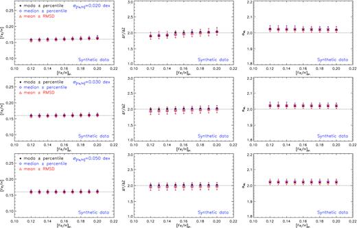
As in Fig. 6, but for TYPE_3 data set.

Open in new tabDownload slide

7 REAL DATA: HYADES CLUSTER

The method, tested in the previous sections, has been applied to the Hyades MS portion with B_P ∈ [3.5,  6.5] mag with the isochrone age fixed to 500 Myr. The uncertainties on the photometry used for the recovery are similar to that discussed for TYPE_1 data set: (1) the absolute B_p magnitude errors take into account the magnitude error given in the original tables plus a systematic uncertainty of 0.01 mag (dominant contribution) due to a possible 0.1 mas zero-point error in the estimated parallax, and (2) for the G − Rp colour index we used the errors in the original tables that range between 0.001 and 0.003 mag (with a mean value of about 0.002 mag). As previously shown, the adopted age is not crucial since the location in the CMD of the selected portion of MS is independent of the adopted age, at least within the range 300–700 Myr. However, to be sure that the results are not affected at all by the adopted age, the recovery was performed also for two other different ages: 300 and 700 Myr. As expected the age variation does not affect the derived values of ΔY/ΔZ, α_ML, and [Fe/H].

Fig. 8 shows the marginalized posterior distributions used to derive the most probable value of [Fe/H], ΔY/ΔZ, and α_ML, for the cases where a Gaussian prior on [Fe/H] is adopted. For the Hyades cluster, spectroscopic measurements of [Fe/H] are available, thus it is recommended to adopt a prior on [Fe/H]. The [Fe/H] value from the literature ranges between +0.10 and +0.20 (see e.g. Cayrel, Cayrel de Strobel & Campbell 1985; Boesgaard & Friel 1990; Paulson, Sneden & Cochran 2003; Schuler et al. 2006; Carrera & Pancino 2011). In particular recent measurements by Dutra-Ferreira et al. (2016) give a best value of [Fe/H] = +0.14 ± 0.03 or +0.18 ± 0.03 dex, depending on the setup used to derive [Fe/H] from the spectra. We adopted these two latter values, which are representative within the uncertainty of ±0.03 dex of both low (+0.13 ÷  + 0.14) and high (up to +0.20) [Fe/H] values measurements present in the literature.

Figure 8.

Posterior marginalized distributions for Hyades data set, for [Fe/H] (left-hand panels), ΔY/ΔZ (mid panels), and α_ML (right-hand panels), for two choices about the Gaussian metallicity prior, namely [Fe/H]_pr = +0.14 dex and σ_FeH = 0.03 dex (top panel), and [Fe/H]_pr = +0.18 dex and σ_FeH = 0.03 dex (bottom panel).

Open in new tabDownload slide

The top panels of Fig. 8 refers to the case where we adopted a prior centred in [Fe/H]_pr = +0.14 with σ_FeH = 0.03. The distributions of [Fe/H], ΔY/ΔZ, and α_ML show a clear peak that can be used to define the most probable value of these parameters. We obtain [Fe/H] = +0.153 with a CI of [+0.125, +0.183], ΔY/ΔZ = 1.91 with the corresponding CI of [1.40, 2.23], and α_ML = 1.99 with CI of [1.94, 2.05].

The results are affected by the adopted prior for [Fe/H]. If one chooses a Gaussian prior with [Fe/H]_pr = +0.18 with σ_FeH = 0.03 one finds different values of the most probable [Fe/H], ΔY/ΔZ, and α_ML, which however are consistent within their CI with the values obtained above. We obtain: [Fe/H] = +0.194 with CI of [0.163, +0.223], ΔY/ΔZ = 2.31 with a CI of [1.89, 2.52], and α_ML = 2.03 with a CI of [1.97, 2.08].

In both the cases, in agreement with the results from the synthetic data set, the parameter derived with the best precision is α_ML: from the analysis, we obtained an α_ML value fully compatible with our solar calibrated mixing length, namely α_ML⊙ = 2.0.

On the other hand, ΔY/ΔZ is recovered with a relatively large CI, and more important, the most probable value depends on the adopted prior on [Fe/H]. For such parameter, the best value changes from ΔY/ΔZ ≈ 2 at [Fe/H]_pr = +0.14 to ΔY/ΔZ ≈ 2.3 at [Fe/H]_pr = +0.18. Given such a dependence of ΔY/ΔZ value on the adopted prior for [Fe/H], we performed an analysis of the effect on the recovered quantities on [Fe/H]_pr, as done in the previous section for the synthetic data sets.

Fig. 9 shows the values of [Fe/H], ΔY/ΔZ, and α_ML obtained using the same grid of [Fe/H]_pr and σ_FeH defined in the previous section. As already noted in the analysis of the mock data set, the most probable value of ΔY/ΔZ varies depending on [Fe/H]_pr and σ_FeH (and on the adopted estimator) in the interval [1.6, 2.6], being subjected to a bias that comes from the adopted prior on [Fe/H]. On the other hand, the mixing length parameter is, as expected, less affected by such bias. As in the synthetic data sets, the most probable value of α_ML varies at maximum of about 2–3 percent for σ_FeH = 0.02 or 0.03 dex, while the maximum variation is a bit larger (about 4–5 percent) for σ_FeH = 0.05 dex.

Figure 9.

Most probable value and corresponding CI for [Fe/H] (first column), ΔY/ΔZ (second column), and α_ML (third column) for Hyades data set, as a function of [Fe/H]_pr and for three values of σ_FeH = 0.02, 0.03, and 0.05 dex (first, second, and third rows, respectively). In figure, we also overplotted the best value and the relative CI obtained using the median and the mean (see the text).

Open in new tabDownload slide

We want to emphasize that not all the [Fe/H]_pr values in figure are equally probable. To be very conservative we adopted a large interval of [Fe/H]_pr, but as already noted, the recent determinations of [Fe/H] for the Hyades cluster suggest – as prior – values in the range [+0.14, +0.18], with an uncertainty of 0.03 dex. If the analysis is restricted to this range of [Fe/H]_pr and to σ_FeH ≤ 0.03 dex, the most probable value of ΔY/ΔZ is in the range [1.7, 2.2] for σ_FeH = 0.02 dex or [1.8, 2.3] for σ_FeH = 0.03 dex. If one takes into account also the (large) CI of the ΔY/ΔZ estimates for these two cases, than the possible ΔY/ΔZ values vary in the interval [1.4, 2.4] for σ_FeH = 0.02 dex and [1.5, 2.5] for σ_FeH = 0.03 dex.

We can define an average value of ΔY/ΔZ, α_ML and also [Fe/H] by considering the values obtained using (1) different estimators, (2) different values of [Fe/H]_pr in [ + 0.14,   + 0.18], and (3) σ_FeH equal to 0.02 and 0.03 dex. If we consider this sample, we obtain <ΔY/ΔZ>=2.03 ± 0.33 and <α_ML>=2.01 ± 0.05 and <[Fe/H]>=+0.169 ± 0.025, which are our best estimate for these parameters using the current set of models. Fig. 10 shows as an example the comparison between the Hyades data and the isochrone computed with a set of parameters, among those available in the grid, as close as possible to the average values of <[Fe/H]>, <ΔY/ΔZ>, and <α_ML>.

Figure 10.

Comparison between Hyades data and the ‘best’ isochrone obtained using a set of parameters among those available in the grid as close as possible to the average values <ΔY/ΔZ>, <α_ML>, and <[Fe/H]> obtained from the analysis.

Open in new tabDownload slide

From the estimated ΔY/ΔZ, we obtained an initial helium content for the Hyades stars Y = 0.2867 (for [Fe/H] = +0.17, Z = 0.01863), which is larger than the solar one. As discussed in the Introduction, in the literature one can find estimates of the Hyades helium content based on different techniques: (1) a binary system (vB22) or (2) MS stars. These two different methods resulted in different helium abundances (Perryman et al. 1998; Lebreton et al. 2001; Castellani et al. 2002; Pinsonneault et al. 2003; Gennaro et al. 2010). In particular, it seems to emerge that when the Hyades MS stars are used, then the derived helium content is compatible with a supersolar value, while the analysis of the vB22 binary systems suggests a lower helium content. The detailed comparison between these results goes beyond the aim of this paper. We limit to say that the results present in the literature were obtained using different methods and different stellar models with different input physics and parameters, which introduce differences and systematics in the derived helium content not easily quantifiable, as discussed in Lebreton et al. (2001) and Pinsonneault et al. (2003). Nevertheless, it would be interesting, for future work, to analyse the difference in the derived helium contend when binary systems or MS Hyades stars are used, but relying on the same set/grid of stellar models.

As a final comment, we notice that the values of <[Fe/H]>, <ΔY/ΔZ>, and <α_ML> clearly depend on the adopted set of models, that is, on the input physics used to generate the tracks/isochrones. Thus the errors on the average values for the parameters derived here are probably an underestimation, because the systematic uncertainty deriving from the adoption of different input physics is not evaluated. Such an analysis, which would require a very huge computational effort, is beyond the scope of this paper, whose aim is to set up the method, test, and analyse its applicability to synthetic data and then apply it to the real data using our reference set of models.

8 CONCLUSIONS

The aim of the paper is to analyse the possibility to precisely calibrate the mixing length parameter α_ML and the helium-to-metal enrichment ratio ΔY/ΔZ adopted in stellar models with the MS of open clusters. The essential precondition for a good performance is the availability of precise photometry, distance, and reddening estimates. Relying on the recent Gaia DR2 data set, we selected the Hyades cluster, which being close, without reddening and having a very good photometry, satisfies all the needed requirements. We restricted our analysis to the Hyades MS in the B_P magnitude range [3.5, 6.5] mag because this region is insensitive to the (‘a priori’ unknown) cluster age and not affected by known problems in matching theoretical colours and observations in low MS.

A Bayesian method is applied to simultaneously derive the set of parameters (namely ΔY/ΔZ, α_ML, and [Fe/H]) that better reproduces the observed MS. We applied the method to a mock data set as close as possible to the Gaia DR2 Hyades data.

We proved that the Bayesian analysis is capable of recovering the most probable value of α_ML with a very good precision, while [Fe/H] and ΔY/ΔZ are correctly determined only when a suitable prior on [Fe/H] is specified. This happens because of the well-known degeneracy [Fe/H]–ΔY/ΔZ which leads to a significant overlapping of the models with different combinations of [Fe/H] and ΔY/ΔZ, thus preventing a good determination of both these parameter when no prior information about [Fe/H] is available, especially when only part of the cluster MS is selected (i.e. in the range B_P ∈ [3.5,  6.5] mag). In this range, we found a relatively large bias in the recovered [Fe/H] and ΔY/ΔZ. Since the sensitivity to a variation of the helium abundance and metallicity on the CMD location of low- and high-mass MS stars is different, a significant improvement of both the accuracy and precision of the results can be achieved if the analysis is extended to a fainter portion of the MS, that is, down to to B_P ∼ 10 mag (M ∼ 0.5 M_⊙). In this case, we proved that beside α_ML, also the recovered ΔY/ΔZand [Fe/H] values are very close to the true ones used to generate the mock data set.

We tested whether the availability of an accurate spectroscopic [Fe/H] value could be used as a prior to restrict the interval of both [Fe/H] and ΔY/ΔZ values. We showed that adopting a Gaussian prior on [Fe/H] we can derive values for [Fe/H], ΔY/ΔZ, and α_ML fully compatible with the true ones used to generate the data set. The best precision is achieved in the recovered value of α_ML (with an uncertainty of 2–3 percent) without any significant bias. Using a reduced portion of the MS, the recovered ΔY/ΔZ value shows a small and negligible bias (ΔY/ΔZ is less than 1 percent smaller than the true one) with an uncertainty of about 10–15 percent. Also [Fe/H] show a negligible bias with an uncertainty that is very close to the dispersion adopted in the Gaussian prior. As in the case of no prior on [Fe/H], the accuracy and precision of the results are improved if the extended MS is adopted: in this case, the bias in ΔY/ΔZ and [Fe/H] reduces to completely negligible values.

We also investigated the dependence of the recovered parameters on the [Fe/H] prior adopted (i.e. [Fe/H]_pr and σ_FeH), only when a portion of the MS is used. The derived [Fe/H] is strictly correlated to [Fe/H]_pr and σ_FeH: the smaller is σ_FeH and greater is the correlation between [Fe/H] and [Fe/H]_pr. Also ΔY/ΔZ is correlated to [Fe/H]_pr, and the inferred ΔY/ΔZ values can differ by about 20–25 percent among each other depending on [Fe/H]_pr: the lower is [Fe/H]_pr and the lower is ΔY/ΔZ. This clearly show that the adoption of a not suitable prior on [Fe/H] leads to the introduction of a bias on the derived quantity. Both for [Fe/H] and ΔY/ΔZ the CI increases if σ_FeH increases: for ΔY/ΔZ we found an uncertainty of about 0.3 (about 15 percent) for σ_FeH = 0.02 dex, which increases to about 0.4–0.5 (about 20–25 percent) for σ_FeH = 0.05 dex. For [Fe/H], the uncertainty is in almost all the cases equal to σ_FeH. On the other hand, α_ML is only marginally affected by the adopted prior on [Fe/H] and the values obtained using different [Fe/H]_pr differs by about 2–3 percent, at maximum.

Finally, we applied the method to the Hyades stars, using a Gaussian prior on [Fe/H] based on recent observational determinations of this quantity. As already noticed, the parameter that is recovered with a very good precision is the mixing length, while ΔY/ΔZ and [Fe/H] are less precise and they are also affected by the adopted [Fe/H]_pr. To obtain a robust estimate of the most probable value of [Fe/H], ΔY/ΔZ, and α_ML, we evaluated these parameters adopting as prior a grid of values of [Fe/H]_pr. Then, we took the average value for each estimated parameter, restricting the average to values of [Fe/H]_pr∈ [ + 0.14,   + 0.18], with σ_FeH = 0.02 and 0.03 dex, which are representative of the most recent determinations of [Fe/H] with the related uncertainty. The obtained results was: <[Fe/H]>=+0.169 ± 0.025, <ΔY/ΔZ>=2.03 ± 0.33 and <α_ML>=2.01 ± 0.05. These tightly calibrated values of the helium-to-metal enrichment ratio ΔY/ΔZ and mixing length parameter α_MLcan be safely adopted to compute the grids of evolutionary tracks required to infer more precisely the stellar parameters of other clusters and field stars.

ACKNOWLEDGEMENTS

The authors thank the anonymous referee for the useful comments that helped to improve the manuscript. ET acknowledges University of Pisa, Dipartimento di Fisica E. Fermi and INAF-OAAb for the fellowship ‘Analisi dell’influenza dell’evoluzione protostellare sull’abbondanza superficiale di elementi leggeri in stelle di piccola massa in fase di pre-sequenza principale’. PGPM and SD acknowledge INFN (iniziativa specifica TAsP).

DATA AVAILABILITY

This work has made use of data from the European Space Agency (ESA) mission Gaia (https://www.cosmos.esa.int/gaia), processed by the Gaia Data Processing and Analysis Consortium (DPAC, https://www.cosmos.esa.int/web/gaia/dpac/consortium). Funding for the DPAC has been provided by national institutions, in particular the institutions participating in the Gaia Multilateral Agreement.

The Hyades data underlying this article were derived from the Gaia DR2 catalogue available at the url: https://gea.esac.esa.int/archive/.

Footnotes

REFERENCES