


ABSTRACT
Binary supermassive black holes (BSBHs) are expected to be a generic byproduct from hierarchical galaxy formation. The final coalescence of BSBHs is thought to be the loudest gravitational wave (GW) siren, yet no confirmed BSBH is known in the GW-dominated regime. While periodic quasars have been proposed as BSBH candidates, the physical origin of the periodicity has been largely uncertain. Here, we report discovery of a periodicity (p = 1607 ± 7 d) at 99.95 per cent significance (with a global p value of ∼10−3 accounting for the look elsewhere effect) in the optical light curves of a redshift 1.53 quasar, SDSS J025214.67−002813.7. Combining archival Sloan Digital Sky Survey data with new, sensitive imaging from the Dark Energy Survey, the total ∼20-yr time baseline spans ∼4.6 cycles of the observed 4.4-yr (rest frame 1.7-yr) periodicity. The light curves are best fit by a bursty model predicted by hydrodynamic simulations of circumbinary accretion discs. The periodicity is likely caused by accretion rate modulation by a milli-parsec BSBH emitting GWs, dynamically coupled to the circumbinary accretion disc. A bursty hydrodynamic variability model is statistically preferred over a smooth, sinusoidal model expected from relativistic Doppler boost, a kinematic effect proposed for PG1302−102. Furthermore, the frequency dependence of the variability amplitudes disfavours Doppler boost, lending independent support to the circumbinary accretion variability hypothesis. Given our detection rate of one BSBH candidate from circumbinary accretion variability out of 625 quasars, it suggests that future large, sensitive synoptic surveys such as the Vera C. Rubin Observatory Legacy Survey of Space and Time may be able to detect hundreds to thousands of candidate BSBHs from circumbinary accretion with direct implications for Laser Interferometer Space Antenna.
1 INTRODUCTION
LIGO has detected gravitational waves (GWs) from stellar-mass binary black hole mergers (Abbott et al. 2016), yet many GW sources are expected outside the LIGO frequency (Sesana 2017; Schutz 2018). A binary supermassive black hole (BSBH) consists of two black holes, each with a mass of ∼106–109 M⊙. BSBHs are expected to frequently form in galaxy mergers (Begelman, Blandford & Rees 1980; Haehnelt & Kauffmann 2002; Volonteri, Haardt & Madau 2003), given that most massive galaxies harbour SMBHs (Kormendy & Richstone 1995; Ferrarese & Ford 2005). Their final coalescences should produce the loudest GW sirens in the universe (Thorne & Braginskii 1976; Haehnelt 1994; Vecchio 1997; Jaffe & Backer 2003), which will be the primary source of low-frequency GW experiments (Amaro-Seoane et al. 2017; Arzoumanian et al. 2018b; Sesana et al. 2018). BSBHs are important for testing general relativity in the strong field regime and for the studies of galaxy evolution and cosmology (Centrella et al. 2010; Merritt 2013; Colpi 2014; Berti et al. 2015).
However, no confirmed case is known at sub-milliparsec scales, i.e. separations close enough to be in the GW-dominated regime. While ∼150 periodic quasars have been suggested as close BSBH candidates (e.g. Valtonen et al. 2008; Graham et al. 2015; Charisi et al. 2016; Liu et al. 2019; Zhu & Thrane 2020), even the most promising candidates are subject to false positives due to quasar’s stochastic, red noise variability, given the limited time baseline and relatively low sensitivity of existing surveys (e.g. see Vaughan et al. 2016 for evidence against any significant periodicity in PG 1302−102 and Goyal et al. 2018 in the case of OJ 287). The study of periodic quasars is important to the searches for close BSBHs in order to test theories of BSBH evolution to shed light on the expected rate of BSBH mergers as GW sources. The study is also important for understanding the physical origin of quasar periodicity, which is largely unknown.
Circumbinary accretion discs are generally expected around close BSBHs at the inferred binary separations of the candidate periodic quasars. Theory suggests that hydrodynamic variability in the circumbinary accretion discs may cause periodic light curves due to accretion rate modulation from the binary torque (e.g. Farris et al. 2014; Gold et al. 2014b; Shi & Krolik 2015; Duffell et al. 2019). This should be useful for finding BSBHs that are close enough to be emitting GWs. However, no evidence has been found for the generic ‘sawtooth’ pattern (i.e. with a sharp rise and a gradual decay, in contrast to a more smooth, sinusoidal modulation expected from Doppler beaming (e.g. D’Orazio et al. 2015a; Duffell et al. 2019), largely limited by the relatively low sensitivity of previous surveys.
In this paper, we present a significant periodicity discovered in the optical light curves of a redshift z = 1.53 quasar, SDSS J025214.67−002813.7 (hereafter J0252 for short). Our systematic search combines new, highly sensitive light curves from the Dark Energy Survey (Dark Energy Survey Collaboration 2016) Supernova (DES-SN) fields (2012–2019; Bernstein et al. 2012; Goldstein et al. 2015; Kessler et al. 2015; Tie et al. 2017) with archival data from the SDSS Stripe 82 (S82) survey (1998–2007; Ivezić et al. 2007). Unlike previous studies, which were based on few-cycle (e.g. ∼1.5) searches, given the limited time baselines, the periodicity of J0252 was discovered based on ∼5 cycles enabled by a ∼20-yr long baseline. The long baseline and high sensitivity are instrumental in rejecting false positives and recovering false negatives caused by stochastic quasar variability (e.g. Vaughan et al. 2016; Barth & Stern 2018). Furthermore, we show that the distinct ‘sawtooth’ pattern (expected from hydrodynamic circumbinary accretion disc variability models) is favoured over a smoother, sinusoidal expected from Doppler beaming (e.g. D’Orazio et al. 2015a; Duffell et al. 2019). In addition, the frequency dependence of the variability amplitudes disfavours Doppler beaming, lending further support to the circumbinary accretion model.
The paper is organized as follows. Section 2 describes the data and methods. Section 3 presents our results on the detection of a significant periodicity in J0252 and its relevant physical properties. We discuss the implications of our results in Section 4 and conclude in Section 5. A concordance ΛCDM cosmology with Ωm = 0.3, ΩΛ = 0.7, and H0 = 70 km s−1 Mpc−1 is assumed throughout. We use the AB magnitude system (Oke 1974) unless otherwise noted.
2 DATA AND METHODS
2.1 Sample selection
We start with 763 spectroscopically confirmed quasars in the 4.6 deg2 overlapping region between the SDSS Stripe 82 survey and the DES-SN fields (S1 and S2). They include 758 objects in the SDSS DR7/DR14 quasar catalogues (Schneider et al. 2007; Pâris et al. 2018) and/or the OzDES quasar catalogue (Childress et al. 2017; Tie et al. 2017), as well as five objects supplemented from the Million Quasars Catalog (Flesch 2015) (v5.5, 2018 November 14). We focus on spectroscopically confirmed quasars to ensure a clean sample in this pilot study. Only point sources are included in the analysis to avoid systematics from host galaxy contamination. We request that the DES flag SPREAD_MODEL <0.005, i.e. the difference between the source point spread function (PSF) and the local PSF model is smaller than 0.5 per cent, or the source PSF is smaller than the local model PSF. We further require that a quasar has at least 30 > 3σ SDSS epochs and 50 DES epochs in at least two bands. The final parent sample consists of 625 quasars. They have a median spectroscopic redshift of ∼1.8 and a median average i-band PSF magnitude of 21.0 mag (AB). The median epoch of observations is 80 from the SDSS and 135 from the DES.
2.2 Light curve data
We combine archival light curves from the SDSS Stripe 82 survey with new observations from the DES-SN fields (described in detail below). The time baseline of the combined light curves extends ∼20 yr (1998–2007 from SDSS Stripe 82 and 2012–2019 from DES-SN). For a typical quasar at z ∼1, the time baseline spans ∼10 yr in the quasar rest frame to encompass ≳5 cycles for a period of ≲2 yr, which is the recommended number of cycles to minimize false periodicity (Vaughan et al. 2016). We have rejected >5σ outliers from the running median in each band. We have binned the data within the same Julian date for a better S/N. We quote AB magnitudes throughout unless otherwise noted.
The DES is a wide-area 5000 deg2 survey of the Southern hemisphere in the grizY bands (Flaugher 2005; The Dark Energy Survey Collaboration 2005; Dark Energy Survey Collaboration 2016). It uses the Dark Energy Camera (Flaugher et al. 2015; Bernstein et al. 2017) with a 2.2-degree diameter field of view mounted at the prime focus of the Victor M. Blanco 4-m telescope on Cerro Tololo in Chile. The typical single-epoch 5σ point source depths (Abbott et al. 2018) are g = 24.3, r = 24.1, i = 23.5, z = 22.9, and Y = 21.4, much deeper than other surveys of larger area (e.g. SDSS and PanSTARRS1). The data quality varies due to seeing and weather variations. The DES absolute photometric calibration has been tied to the spectrophotometric Hubble CALSPEC standard star C26202 and has been placed on the AB system (Oke & Gunn 1983), with an estimated single-epoch photometric statistical precision of 7.3, 6.1, 5.9, 7.3, 7.8 mmag in grizY bands (Abbott et al. 2018). The DES contains a 30 deg2 multiepoch survey (DES-SN) to search for SNe Ia that has a mean cadence of ∼7 d in the griz bands. Two of the 10 DES-SN fields (S1 and S2) are overlapped with the SDSS Stripe 82 (with an overlapping area of 4.6 deg2). We adopt light curves generated from the Y6A1 Gold data (Morganson et al. 2018). We have also included the Science Verification data to maximize the time baseline.
The SDSS equatorial Stripe 82 region was observed from 1998 September to 2007 December with ∼70–90 total epochs of images in the ugriz bands obtained in yearly ‘seasons’ about 2–3 months long (Adelman-McCarthy et al. 2007; Ivezić et al. 2007; Frieman et al. 2008). The typical single epoch 5σ point source depths are 22.2, 22.2, 21.3, and 20.5 in the griz bands (Adelman-McCarthy et al. 2007). The photometric calibration over the survey area is accurate to roughly 0.02 mag in the gri bands, and 0.03 mag in the uz bands (Ivezić et al. 2004). All SDSS magnitudes have been calibrated to be nearly on the AB system (Abazajian et al. 2009).
J0252 is a spectroscopically confirmed quasar contained in the SDSS DR14 quasar catalogue (Pâris et al. 2018). Fig. 1 shows its griz multicolour optical light curves. The ∼20-yr observations combine archival SDSS data with new, higher signal-to-noise imaging from DES. The SDSS (DES) observations included 83, 83, 84, and 85 epochs (131, 140, 141, and 143 epochs) in the griz bands with a median separation of 4 d (7 d) between epochs and yearly seasonal gaps. The variability of J0252 is more coherent with a larger amplitude than typically observed for stochastic quasar variability (Morganson et al. 2014) generally believed to result from thermal fluctuations in the accretion discs driven by an underlying stochastic process such as a turbulent magnetic field.
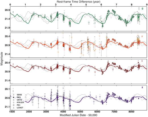
SDSS and DES optical light curves of J0252. All observations have been corrected to be on the DES system. Also shown are archival light curves from the PTF, CRTS, ZTF, PS1, and new observations from the LCOGT. Error bars represent 1σ (statistical). The solid curves show the best-fitting models from hydrodynamic circumbinary accretion disc simulations assuming a mass ratio q = 0.11 (Farris et al. 2014), of which the thick solid denotes our baseline model assuming a background of random, red noise variability whereas the thin solid assumes white (flat spectrum) noise for comparison purposes only. Note that because we assume red noise in our baseline model for the background signal (from stochastic variability), the residual is not supposed to be zero, unlike the case of a white noise background. Also shown for comparison are a q = 0.43 accretion model (dotted grey) and a sinusoidal model (dashed grey) expected from Doppler boost (D’Orazio, Haiman & Schiminovich 2015b) both assuming red noise.
Fig. 1 also shows archival photometry from the Palomar Transient Factory (PTF), Panoramic Survey Telescope and Rapid Response System (Pan-STARRS or PS1), and Zwicky Transient Facility (ZTF) survey, as well as our new observations from the Las Cumbres Observatory Global Telescope (LCOGT; DDT Program 2018B-004 and NOAO Program 2019A-0279; PI Liu). This is for the purposes of independent double checks only. We do not include them in our baseline analysis to: (1) ensure homogeneity for the analysis of the parent sample and (2) minimize possible uncertainties and/or caveats in the available data as we describe below. However, we have also verified that our results do not change qualitatively even when including them in the analysis. Further details of the archival photometry can be found in Appendix A, with photometry data provided in the supplementary online data.
2.3 Periodicity detection
For any periodicity detection, we implement the following three selection criteria:
At least two bands have a 3σ detection of the same periodicity in the periodogram analysis.
The detected periodicity is the dominant component compared to the background noise.
The same periodicity is also identified in the auto-correlation function (ACF).
First, we adopt the generalized Lomb-Scargle (GLS) periodogram (Zechmeister & Kürster 2009), which is appropriate for detecting periodicity in unevenly sampled data using the astroML package (Vanderplas et al. 2012). Comparing the observed power to that from the simulated light curves (see details below), we identify a significant periodicity candidate if at least two bands show a 3σ detection (i.e. the detected periodicity cannot be reproduced by |$\gt 99.7 {{\ \rm per\ cent}}$| synthetic light curves) in the same periodicity grid window. To quantify the statistical significance of any periodogram peak, we adopt an approach similar to that of Charisi et al. (2016). Since the noise spectrum is frequency-dependent (due to the stochastic red noise quasar variability), it is more appropriate to quantify the statistical significance at a given frequency, i.e. as compared to the local background. Adopting a false-alarm probability that is flat over different frequencies instead would overestimate the true statistical significance of periodogram peaks (Liu et al. 2015). In addition, we reject any detection where fewer than three cycles are spanned by the observations or where the periodicity is shorter than 500 d. The former criterion is imposed to minimize false periodicity due to the stochastic red noise quasar variability (Vaughan et al. 2016), whereas the latter is to mitigate artefacts caused by seasonal gaps and low-cadence sampling on short time-scales (i.e. an aliasing effect, e.g. MacLeod et al. 2010).
Secondly, we fit a sine curve to the selected candidates and reject any of them if the residue noise dominates over the periodicity signal, i.e. if |$\sigma _{\rm residue}^2 / A_{\rm sin}^2 \gt 1$|, where Asin is the periodicity amplitude and |$\sigma _{\rm residue}^2$| is the variance of the residue light curve after subtracting the periodic signal. Finally, as a complementary test, we search for periodicity by fitting the ACF with the ZDCF package (Alexander 1997). For a periodicity on top of a stochastic background, ACF has a damped periodic oscillation with ACF(t) = cos (ωt)exp (− λt), where t is the lagging time, |$\omega = \frac{2 \pi }{P}$|, and λ is the decay rate of the stochastic background (Graham et al. 2015). We require that the GLS periodicity be consistent with that from the ACF test. Besides the above criteria, we have tested alternatives using the multiband GLS by VanderPlas & Ivezić (2015) and the modified GLS adopted by Zheng et al. (2016) and found that they provide no further constraint in our candidate selection, i.e. the candidates selected by the three criteria also have 3σ detections in these alternative methods.
2.4 Simulated light curves
To quantify the statistical significance of any periodicity, first we generate 50 000 evenly sampled mocked light curves assuming a damped random walk (DRW) model with variability parameters tailored to the observed properties of each quasar. A DRW model uses a self-correcting term added to a random walk model that acts to push any deviations back towards the mean. It captures the stochastic properties of quasar variability on a time-scale ≳10 d (Kelly, Bechtold & Siemiginowska 2009; MacLeod et al. 2010; Mushotzky et al. 2011; Kozłowski 2016; Smith et al. 2018). The DRW model is known as a red noise model, which has a higher spectrum power in lower frequencies. Models that failed to account for this red noise feature would likely identify false positives due to the generic power spectrum feature. The DRW model is governed by two parameters: σ2 and τ, which describe the flux variance and correlation time-scale of the variability.
To measure the DRW parameters and uncertainties for each quasar, we fit the light curve directly in the time domain by treating each data point as a state space with a Gaussian uncertainty due to both the stochastic process and measurement error, following equations (6)–(12) of Kelly et al. (2009). For unevenly sampled data, fitting the light curve directly in the time domain is preferred over fitting the power spectrum density for better recovering the true DRW parameters. The structure function due to the observational cadence may induce an anomalous power in the power spectrum that could potentially bias the fitting result. We apply a Bayesian model using the Markov Chain Monte Carlo (MCMC) method with the emcee package adopting a non-informative prior (Foreman-Mackey et al. 2013). The fitting starts with 200 walkers and samples for 1500 steps. The first 750 steps are removed as a burn-in process. To test for the convergence, we repeat the above processes but with only half of the steps (750 steps), and the resulting parameter distribution is consistent. Fig. 2 shows the parameter estimation. For J0252, we have also tested a different prior with a lognormal distribution centred at 0.08 mag and 200 d for σ and τ, respectively, with a standard deviation of 1.15 (Kelly et al. 2009; MacLeod et al. 2010). The analysis is consistent across different choices of prior.
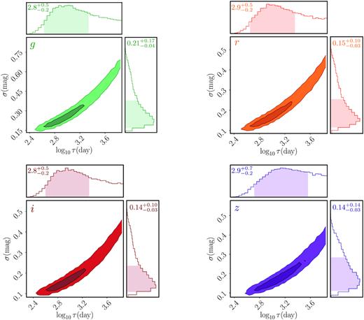
DRW model parameter estimates for J0252. The 2D contours show the 68 per cent and 95 per cent confidence levels estimated from the MCMC analysis. The histograms show the projected 1D probability density distributions for σ and τ (observed frame). Labelled on each panel are their best-fitting value and the 1-σ (estimated from the 68 per cent confidence levels denoted by the shaded histograms) uncertainties. The total light-curve baseline (∼7300 d) is more than 10 times larger than the correlation time-scale (∼630 d in observed frame), so that the correlation time-scale recovers the true value (Kozłowski 2017).
Fig. 2 shows the best-fitting DRW parameters for J0252. We have verified that the light-curve baseline (∼7300 d) is more than 10 times larger than the correlation time-scale (∼630 d in the observed frame), so that the correlation time-scale recovers the true value (Kozłowski 2017). We then generate 50 000 mock light curves with parameters pairs (σ2 and τ) randomly drawn from the posterior distribution in the DRW parameter fitting. We down sample the mock light curves to match the cadence of the observations and add measurement errors.
We also consider a bending power-law (BPL) model as an alternative to the DRW model assumption for the simulated light curves. This is motivated by results based on high-cadence Kepler observations that suggest deviations from the DRW model at the high-frequency end |$f \gtrsim \frac{1}{10}$| d−1 (Mushotzky et al. 2011; Edelson et al. 2013, 2014; Smith et al. 2018). For the BPL model, we assume a −3 power spectrum index at the high frequency |$f \gt \frac{1}{10}$| d−1 and keep the DRW model at the low frequency |$f \lt \frac{1}{10}$| d−1. We have tested different power-law indices and different high-frequency breaks. Our result is insensitive to these choices. The low-frequency breaks are drawn from the time-scales τ in the DRW parameter fitting. We first generate 50 000 evenly sampled mocked light curves assuming the BPL model with the pyLCSIM1 package. We then down sample the light curve and measure the power spectrum density using the GLS periodogram. Our result is consistent with that assuming a pure DRW model.
In addition to the DRW model, we have also considered the CAR(2,1) model (Kelly et al. 2014), i.e. a damped harmonic oscillator. CAR(2,1) is often used to describe a periodic signal (Graham et al. 2015; Moreno et al. 2019). The quality factor Q, defined as the ratio of the detected frequency to the corresponding frequency width, is used as a measure of the significance level. For J0252, we have Q ≪ 1 for the CAR(2,1) model, which could suggest a low-significance level for the detected period or a higher order noise. We have tested that the significance of the periodic signal decreases when we assume the CAR(2, 1) model for the ‘stochastic’ component instead of a DRW, although a |$\gt 99.74{{\ \rm per\ cent}}$| detection holds in the g band. Table 1 shows that using carma-pack,2 CAR(1,0) has the lowest BIC value and is thus a proper noise model.
BIC values for CAR(p,q) model using g-band data with p ≤ 3 and q < p. CAR(1,0) has the smallest BIC value, suggesting that DRW is the proper noise model for J0252.
| CAR(p, q) | (1,0) | (2,0) | (2,1) | (3,0) | (3,1) | (3,2) |
|---|---|---|---|---|---|---|
| BIC | −967 | −927 | −922 | −917 | −920 | −906 |
| CAR(p, q) | (1,0) | (2,0) | (2,1) | (3,0) | (3,1) | (3,2) |
|---|---|---|---|---|---|---|
| BIC | −967 | −927 | −922 | −917 | −920 | −906 |
2.5 eBOSS spectrum and analysis
J0252 has an optical spectrum available from the SDSS DR14 data archive (Plate = 7820, Fiber ID = 470, MJD = 56984). It was taken by the BOSS spectrograph within the SDSS-IV/eBOSS survey (Dawson et al. 2016). The BOSS spectrum covers 3650–10400 Å with a spectral resolution of R =1850–2200. Fig. 3 shows its optical (rest-frame UV) spectrum, where multiple broad emission lines are detected including C iv λ1549, He ii λ1640, C iii] λ1909, and Mg ii λ2800.
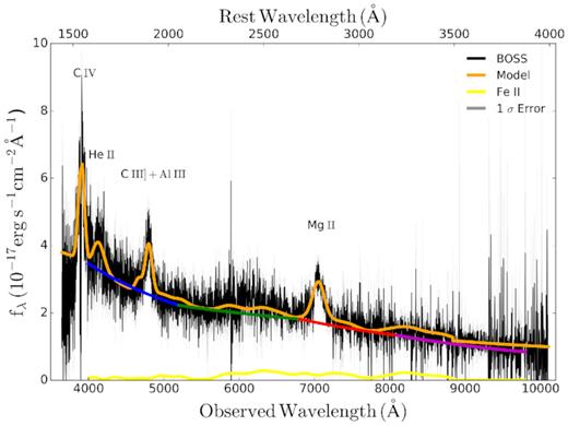
Optical spectrum and modelling of J0252. Shown are the data (black), the 1-σ error (grey), the best-fitting model (orange), the Fe II pseudo-continuum (yellow), and the broken power-law model for the emission-line- and Fe II-subtracted continuum (with the griz bands plotted in blue, green, red, and magenta, respectively).
To estimate the viral black hole mass from the broad emission lines, we follow the procedure described in Shen & Liu (2012) and Shen et al. (2019) by fitting the spectral models to the observed spectra. The spectral models contain a linear combination of power-law continuum, a pseudo-continuum generated from Fe II emission templates, and single or multiple Gaussian components for the emission lines. Since the errors in the continuum model might change the fitting of the weak emission lines, we perform a global fit to the mission-line free region first to construct the continuum model better. Then, we fit multiple Gaussian models to the emission lines around the Mg ii λ2800 region locally. The Mg ii λ2800 line is fitted by a combination of up to two Gaussians for the broad component and one Gaussian for the narrow component. For the full width at half-maximum of the narrow lines, we also impose an upper limit of 1200 km s−1. Fig. 3 shows our spectral models for J0252.
3 RESULTS
3.1 Discovery of a significant periodicity in J0252
Using the three criteria described in Section 2.3, we identify five significant periodic candidates out of the parent sample of 625 quasars in a 4.6 deg2 field. J0252 was the most significant detection with >4 cycles spanned whose light curves prefer a bursty circumbinary accretion model. We focus on J0252 in this paper, whereas the other four candidates are presented in Chen et al. (2020).
Fig. 4 shows the GLS periodogram (Zechmeister & Kürster 2009). An observed 4.4-yr (corresponding to rest frame 1.7 yr at the redshift of 1.53) periodicity is detected at 99.95 per cent, 99.43 per cent, 99.78 per cent, and 99.59 per cent single-peak significance in the griz bands. The empirically estimated global p values (Barth & Stern 2018) are 1.2 × 10⁻³, 5.8 × 10⁻³, 2.6 × 10⁻³, and 8.4 × 10⁻³, accounting for the look elsewhere effect (e.g. Gross & Vitells 2010) in the whole frequency range being searched (see Chen et al. 2020, for details). The confidence level in each band was determined from 50,000 Monte Carlo simulations (described in Section 2.4) tailored to the observed variability flux variance and characteristic time-scale assuming a DRW (Kelly et al. 2009) or a more general BPL model. There is a ∼0.1 per cent probability that the periodogram peak is produced by stochastic quasar variability (i.e. assuming a correlated red noise), but the fact that we have found five candidates at >99.74 per cent single-peak significance in a parent sample of 625 (in which ≲2 cases are expected from red noise; Chen et al. 2020) suggests that we are not just seeing stochastic quasar variability in our small sample. Similar to Figs 4 and 5 shows the significance level assuming a CAR(2,1) noise. The candidate periodicity is found at 99.8 per cent, 98.8 per cent, 99.5 per cent, and 98.0 per cent single-peak significance in the griz bands under the CAR(2,1) assumption for the stochastic noise. For context, the false alarm probability of seeing such a significant peak in the periodograms is ≪10−20 assuming a pure white (i.e. flat spectrum) noise instead (Zechmeister & Kürster 2009). Chen et al. (2020) have estimated the DRW parameter distributions for the parent quasar sample to address the false alarm probability for the candidates as a population.
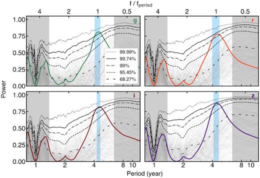
Generalized Lomb-Scargle periodogram showing the periodicity detection of J0252. A periodicity (see PGLS in Table 2) is detected at 99.95 per cent, 99.43 per cent, 99.78 per cent, and 99.59 per cent single-peak significance (with global p values of 1.2 × 10⁻³, 5.8 × 10⁻³, 2.6 × 10⁻³, and 8.4 × 10⁻³ accounting for the look elsewhere effect in the whole frequency range being searched; Chen et al. 2020) in the griz bands. The confidence levels are calculated from 50 000 tailored simulations assuming random, red noise variability. The grey curves show 200 examples drawn from the 50 000 for clarity. The cyan shaded region indicates the period uncertainty estimated using ranges above the >99.74 per cent significance for the gi bands and above the >99.00 per cent significance for the rz bands. The grey shaded regions mark the small time-scales (<500 d) on which a periodicity may be subject to artefacts due to seasonal gaps and low cadence, and the large time-scales (defined as total time baseline <3 cycles) where the data are more subject to false periodicity from stochastic quasar variability (Vaughan et al. 2016).

Archival observations from the PTF (in the gR bands) and from the Pan-STARRS (in the griz bands) provide independent verification of our baseline observations. They also partially filled the cadence gap between the SDSS and DES observations. New observations from the LCOGT and the ZTF provide independent support and verification to our baseline DES observations. Despite having significant gaps, the combined time baseline spans ∼4.6 cycles of the periodicity, approaching the number of observed cycles recommended for minimizing false positives from stochastic quasar variability (e.g. Vaughan et al. 2016).
3.2 Black hole mass estimation
The black hole mass is estimated using the single-epoch spectrum by assuming virialized motion in the broad-line region clouds (Shen 2013). The broad-line region gas clouds would see the candidate BSBH as a single source. From the spectral fit to the eBOSS spectrum, the Mg ii λ2800-based estimator gives a virial black hole mass of |$M = 10^{8.4\pm 0.1} \, \mathrm{M}_{\odot }$| (1σ statistical error), using the parameters in Vestergaard & Osmer (2009). Shen (2013) suggests that Mg ii λ2800-based masses are more reliable than C iv λ1549-based masses, given that C iv λ1549 is likely to suffer from non-virial motion like outflows and there is larger scatter between C iv λ1549 and Hβ masses for quasars at high redshift (Shen & Liu 2012).
3.3 Radio loudness upper limit
J0252 was undetected by FIRST (Becker, White & Helfand 1995) with a 3σ flux density upper limit of <0.5 mJy at 1.4 GHz. It was covered by the VLA Sky Survey (Villarreal Hernández & Andernach 2018) (VLASS) footprint at 3 GHz to a sensitivity of 0.12 mJy rms. It was also undetected by VLASS according to its quicklook image,3 suggesting a 3σ upper limit of |$f^{{\rm obs}}_{{3\, {\rm GHz}}} \lt 0.36$| mJy. Assuming that the radio flux follows a power law fν ∝ να, this translates into |$f^{{\rm rest}}_{{6\, {\rm cm}}} \lt {0.18}$| mJy (6 cm corresponding to 5 GHz) for a spectral index α = −0.5 (Jiang et al. 2007), or |$f^{{\rm rest}}_{{6\, {\rm cm}}}\lt {0.20}$| mJy assuming α = −0.8 (Gibson, Brandt & Schneider 2008). Combining the f2500 measurement from the optical spectrum, the inferred radio loudness parameter (Kellermann et al. 1989) is |$R\equiv f_{{6\, {\rm cm}}/f_{{\rm 2500}}} \lt {14}$| assuming α = −0.5, or R < 15 assuming α = −0.8. While the VLASS upper limit cannot exclude the possibility of J0252 being radio loud (i.e. R > 10 according to the traditional definition based on PG quasars), it does rule out its optical emission being dominated by emission from a radio jet [i.e. R > 100 (Chiaberge & Marconi 2011)].
3.4 Spectral energy distribution
Fig. 6 shows the spectral energy distribution (SED) of J0252. It is similar to a control sample of ordinary optically selected SDSS quasars that are matched in redshift and luminosity. The available SED observations include a radio flux density upper limit from the VLASS, MIR photometry from WISE (Wright et al. 2010), NIR photometry from UKIDSS (Lawrence et al. 2007), optical photometry from the SDSS (York et al. 2000) and an optical spectrum from eBOSS, UV photometry from GALEX (Martin et al. 2005) [including a detection in the near-ultraviolet (NUV) and an upper limit in the far-ultraviolet (FUV)], and an X-ray upper limit from ROSAT (Voges et al. 2000).
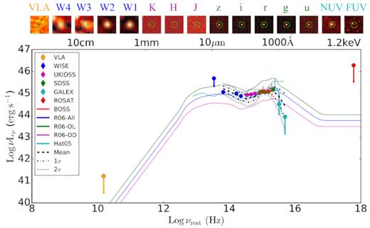
Spectral energy distribution (SED) of J0252. Also shown for comparison are the mean and 1σ and 2σ confidence levels of the SEDs of a control quasar sample matched in redshift and luminosity with J0252, the optically selected quasar SEDs from (Richards et al. 2006) (‘R06-All’ for all quasars, ‘R06-OL’ for optically luminous quasars, and ‘R06-OD’ for optically dim quasars), and the mean SED of (Hatziminaoglou et al. 2005) (Hat05). Error bars are 1σ whereas upper limits are 3σ. Plotted on top are the multiwavelength postage stamps of J0252 with a FOV of 30″ each. The green circles are 10″ in diameter indicating the position of J0252.
A generic prediction from circumbinary accretion disc simulations is a flux deficit in the optical/UV SED. The flux deficit may be a cutoff from a central cavity opened by the secondary black hole (Milosavljević & Phinney 2005) or a notch from minidiscs formed around both black holes (Roedig, Krolik & Miller 2014; Farris et al. 2015). There is tentative evidence for an NUV deficit compared to the control sample from the existing optical spectroscopy and GALEX UV photometry, but the existing data are too uncertain to draw a firm conclusion. Future HST UV spectroscopy could confirm the potential UV deficit as a complementary test of circumbinary accretion disc models.
4 DISCUSSION
4.1 Physical origins of the periodicity
In addition to a pure stochastic quasar variability (i.e. the null hypothesis), we consider two common, competing models for the optical light-curve periodicity. The first is a smooth, sinusoidal model, which is expected from Doppler boosting. It has been proposed to explain the periodic quasar candidate PG1302−102 (D’Orazio et al. 2015b). The highly relativistic motion of the secondary black hole drives an apparent periodicity in the light curve, assuming that the optical emission is dominated by contribution from a mini accretion disc fuelling the secondary black hole.
The second is a more bursty, quasi-periodic variability model predicted by hydrodynamic simulations of circumbinary accretion discs. We adopt the bursty hydrodynamic circumbinary accretion disc variability model of Farris et al. (2014). The model was generated from two-dimensional (2D) hydrodynamical simulations of circumbinary disc accretion using the finite-volume code DISCO (Duffell 2016). It solves the 2D viscous Navier–Stokes equations on a high-resolution moving mesh. The moving mesh shears with the fluid flow and thereby reduces the advection error in comparison to a fixed grid. Unlike previous simulations that have excised the innermost region surrounding the binary by imposing an inner boundary condition, and so potentially neglecting important dynamics occurring inside the excised region, the model was the first 2D study to include the inner cavity using shock-capturing Godunov-type methods. The simulations last longer than a viscous time such that the solutions represent a quasi-steady accretion state.
More specifically, we consider two models, mass ratio q = 0.11 and q = 0.43. These two values are chosen because they represent two characteristic regimes in the light-curve behaviours (fig. 9 of Farris et al. 2014). In the simulations, significant periodicity in the accretion rates emerges only for q ≳0.1, where the binary torques are large enough to excite eccentricity in the inner cavity and create an overdense lump. The passing BHs interact with the overdense lump, producing periodicity in the accretion rate. There is a strong peak in the periodograms corresponding to the orbital frequency of the lump, which is also the binary frequency for q = 0.11 but is ∼1/5 of the binary frequency for q = 0.43. The quality of the existing light curves does not justify model comparison over an even finer parameter grid in mass ratio.
One caveat is that the 2D models predict only the accretion rate and miss 3D effects and radiative transfer processes. While more realistic simulations are still needed to capture the complex physics in the binary system in order to make reliable predictions, the dominant characteristic time-scale, the orbital period, and harmonics that might arise should emerge in the light curve. The gas has to be accelerated by the binary potential, and the emission of the gas has to reflect, at some level, this behaviour. Whether or not we can get an accurate estimate of the mass ratio is indeed uncertain, but circumbinary accretion variability is still preferred over relativistic Doppler boosting both for the more bursty light curve characteristic and the frequency-dependent variability amplitudes as discussed further below.
4.2 Light-curve model fitting and model comparison
We have shown that a periodic model is preferred over a correlated red noise (i.e. modelled with a DRW model) based on the periodogram analysis using tailored simulations (Fig. 4). As an independent analysis, here we also fit the light curve with a covariance matrix that includes a correlated red noise between measurements. It allows us to test if the data favour an additional periodic signal on top of a background of pure random, red noise variability (i.e. from stochastic quasar variability), as well as to perform a comparison between a smooth, sinusoidal model and the more bursty accretion models.
First, we test if the q = 0.11 model could explain our detected periodicity by maximizing the likelihood function without any limitation on the parameters. We use the emcee package to determine the best-fitting parameters and their uncertainties. We initiate 100 individual chains to sample the maximum likelihood function for 500 steps. Then, we remove the first 250 steps as a burn-in process. The 1σ error is determined by the remaining 250 steps from 100 chains at the 84.14 and 15.86 percentiles. The best-fitting q = 0.11 bursty model period along with the 1σ error is listed in Table 2, consistent with the periodicity found in the periodogram analysis.
Measurements of J0252. Line (1): Period and 1σ error (estimated from bootstrap re-sampling) from the generalized Lomb-Scargle (GLS) periodogram. Line (2): Best-fitting period and 1σ error (statistical) from MCMC fitting the q = 0.11 accretion model independently in different bands assuming a correlated red noise. Lines (3)–(5): Bayesian information criterion (BIC) differences between a periodic model and the null hypothesis, i.e. stochastic quasar variability characterized by a damped random walk (DRW) model. The periodic models considered include two bursty, circumbinary accretion models assuming q = 0.11 and 0.43, and a sinusoidal model (expected for relativistic Doppler boost). A negative ΔBIC indicates that a periodic model is more preferred over a pure stochastic variability. ΔBIC < −10 suggests strong evidence. Line (6): Number of data points. Line (7): Power-law index of the continuum from spectral modelling. Errors represent 1σ uncertainties generated from 100 Monte Carlo simulations. Line (8): Variability amplitude from the best-fitting sinusoidal model. Errors represent 1σ statistical uncertainties. Line (9): Best-fitting correlation time in the DRW model. Line (10): Number of free parameters for each of the model.
| Parameter | g | r | i | z | griz |
|---|---|---|---|---|---|
| PGLS (d)........................(1) | 1607 ± 7 | 1615 ± 9 | 1632 ± 8 | 1607 ± 10 | – |
| |$P_{{\rm Acc,\, q = 0.11}}$| (d)........................(2) | 1511|$^{+34}_{-55}$| | 1466|$^{+64}_{-12}$| | 1506|$^{+128}_{-61}$| | 1562|$^{+248}_{-99}$| | 1476|$^{+128}_{-5}$| |
| BIC|$_{{\rm Acc,\, q = 0.11}}$| − BICDRW........................(3) | −19.7 | −23.7 | −13.3 | −13.7 | −96.7 |
| BIC|$_{{\rm Acc,\, q = 0.43}}$| − BICDRW........................(4) | −9.7 | −7.0 | −2.5 | −1.9 | −78.3 |
| BICsin − BICDRW........................(5) | −5.5 | −5.7 | +0.9 | −2.9 | −47.2 |
| N ........................(6) | 212 | 223 | 222 | 227 | 884 |
| α ≡ dln(Fν)/dln(ν)........................(7) | −0.32 ± 0.40 | −1.25 ± 0.34 | −0.20 ± 0.34 | 0.41 ± 1.01 | – |
| Aobs (mag)........................(8) | 0.229 ± 0.003 | 0.162 ± 0.002 | 0.162 ± 0.002 | 0.157 ± 0.004 | – |
| τDRW (d) ........................(9) | 653 | 716 | 629 | 849 | 701 |
| kDRW / kq = 0.11 / kq = 0.43 / ksin....(10) | 3/6/6/6 | 3/6/6/6 | 3/6/6/6 | 3/6/6/6 | 9/15/15/15 |
Then, we compare three models (sinusoidal + red noise, circumbinary accretion + red noise, and a pure stochastic red noise) using maximum likelihood estimation. All the calculations are done in flux units. In a single-band fit, the sinusoidal model has six free parameters: red noise amplitude, red noise correlation time, period, phase, amplitude, and average magnitude. The more bursty, circumbinary disc accretion variability model also has six free parameters: red noise amplitude, red noise correlation time, period, phase shift, amplitude of variation, and the magnitude zero-point. A DRW model has three free parameters: red noise amplitude, red noise correlation time, and mean magnitude.
We also do a combined fit making use of the light curves from all four bands. To help break parameter degeneracy, the periodicity, phase, and red noise correlation time-scale are fixed to be the same across different bands. In a combined fit with the periodic models, we have 15 free parameters, including the mean flux, model amplitude, and red noise amplitude in each band, as well as the periodicity, the phase, and the red noise correlation time-scale, which are the same across different bands. For the pure DRW model, there are nine model parameters, including the mean flux and the red noise amplitude in each band, and a red noise correlation time, which is the same across different bands.
Table 2 lists the BIC from our MCMC analysis for the model fitting and comparisons. Three periodic models are compared against the null hypothesis of a pure stochastic variability. A lower BIC value indicates the more preferred model, and a BIC difference of <−10 suggests strong evidence. In each band, the q = 0.11 accretion model always has a negative BIC difference (i.e. suggesting that it is more preferred than a pure stochastic variability), which is also the smallest among all the three periodic models considered. The observed light curves of J0252 statistically prefer the q = 0.11 accretion model over the other models in all four bands. Taking the fit that combines all bands, for example, the BIC difference between the q = 0.11 accretion model and the pure stochastic quasar variability model translates to a likelihood ratio of, at least, exp[(−96.7)/(−2)] ∼ 1021 (equation 4). We thus conclude the q = 0.11 accretion model to be the best model for the observed light curves.
We have tested that our qualitative conclusion (that the q = 0.11 accretion model is preferred over a sinusoidal model from having smaller BIC values) still holds assuming a background of pure white (flat spectrum) noise instead (i.e. with zero off-diagonal terms in the covariance matrix). We show the best-fitting q = 0.11 accretion models under white noise (thin solid curves) in Fig. 1 for illustration purposes only. We have also tested an eccentric Doppler boost model, but the q = 0.11 circumbinary accretion model still has the lowest BIC.
4.3 Relativistic Doppler boost modelling
The multiband light curves enable us to conduct an independent, quantitative test of the relativistic Doppler boost hypothesis. The relativistic Doppler boost predicts unique and robust frequency-dependent variability amplitudes in different bands that can be tested with multicolour data (D’Orazio et al. 2015b). We adopt the total mass of the hypothesized binary in J0252 as |$M = 10^{8.4\pm 0.1} \, \mathrm{M}_{\odot }$| (1σ statistical error) assuming the virial black hole mass estimated from Mg ii λ2800. We measure the spectral indices of the continuum by fitting broken power-law models over four wavelength windows corresponding to the griz bands. Table 2 lists the resulting broken power-law indices.
We calculate the frequency-dependent variability amplitude ratios expected from relativistic Doppler boost (i.e. relativistic beaming, or RB for short) to compare with the observations. Taking the gr bands, for example, the RB model predicts Ag, RB/Ar, RB = (3 − αg)/(3 − αr) = 0.78 ± 0.11 (1σ), where α ≡ dln(Fν)/dln(ν). The observed Ag, obs/Ar, obs is 1.41 ± 0.03. The RB hypothesis is therefore ruled out at ≳5σ.
Fig. 7 shows the observed variability amplitude ratio (Ai/Aj where i and j represent two bands) compared with the expected value inferred from RB for each band pair, which is (3 − αi)/(3 − αj). The RB model is being ruled out at ≳5σ considering the gr bands and at ∼2σ for the gi and ri bands.
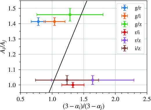
Observed frequency-dependent variability amplitude ratio for each band combination compared with the expected values from relativistic Doppler boost. The black line represents the 1-to-1 relation. Error bars denote 1σ uncertainties.
Fig. 8 shows the parameter space that allows for a flux variability greater than a fiducial value of 16 per cent to 23 per cent in order to explain the observed values (Table 2). The parameters considered are the total black hole mass M, mass ratio q, orbital inclination i, and the fraction of the total emission coming from the secondary black hole f2 (D’Orazio et al. 2015b). Our other fiducial model parameters are Porb = 1.7 yr, and α = −0.32, −1.25, −0.20, and 0.41 in the griz bands (Table 2). There is little to no parameter space for the RB hypothesis to work, because the required total black hole mass would be too large to reproduce the observed, large variability amplitudes in J0252, unless all the following three requirements are met: (1) the total black hole mass is significantly underestimated by the virial estimate, even when accounting for a 0.5-dex systematic uncertainty (Shen 2013), (2) >80 per cent of the optical light is contributed by emission from a mini accretion disc fuelling the secondary black hole, and (3) the system is viewed close to being edge-on.
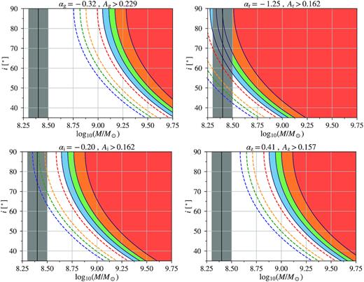
Parameter space estimates for the relativistic Doppler boost model. The four panels represent griz bands. In each panel, the dashed contours represent f2 = 1.0 whereas the shaded contours denote f2 = 0.8, where f2 is the fraction of the total emission coming from the secondary black hole. Different colours show different mass ratios with q = 0.0, 0.05, 0.1, and 0.2 for blue, green, orange, and red, respectively. The vertical solid line with grey shades indicates our virial mass estimate and its 1σ statistical error for the total black hole mass. The orbital inclination angle i = 90 degrees for an edge-on view, and 0 degree for a face-on view.
Our estimates on the periodic variability amplitudes (line 8 in Table 2) do not include contribution from a stochastic background of red noise; accounting for all the observed variability amplitudes instead would make the tension even stronger.
4.4 Gravitational-wave implications and prospects
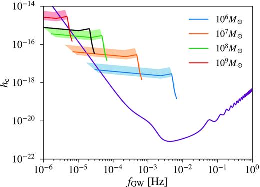
Prospect for LISA detection of a source similar to the candidate BSBH in J0252 but 5 yr before coalescence. The purple curve represents the expected LISA sensitivity limit assuming a 5-yr observation (Cornish & Robson 2018). The black curve denotes the gravitational-wave signal of a BSBH at z = 1.53 with mass 108.4M⊙ and mass ratio q = 0.1 beginning at 5 yr before coalescence, i.e. from the inspiral phase (low frequency) to the final merger and ringdown (high frequency). The blue, orange, green, and red shaded regions correspond to mergers with a primary mass of 106M⊙, 107M⊙, 108M⊙, and 109M⊙, respectively, at the same redshift with mass ratios ranging within 0.05 ≤ q ≤ 0.5. The blue, orange, green, and red lines correspond to q = 0.1.
4.5 Alternative interpretations
Unlike the two previously best known BSBH candidates OJ287 and PG1302, J0252 is not a blazar, nor is its optical emission dominated by contribution from a radio jet, and therefore jet precession cannot explain the periodicity. Precession of a warped accretion disc is unlikely because the amount of obscured continuum emission required would be too large to explain the observed variability amplitude in J0252 and that the effect is geometrical rather than bursty. The periodicity in J0252 (i.e. rest frame 1.7 yr) is close to the expected value (∼200 d) inferred from its black hole mass assuming a scaled-up quasar version (King et al. 2013) of low-frequency accretion disc quasi-periodic oscillations (QPOs; e.g. from strong resonances in the accretion flow) as seen in the X-ray light curves of X-ray binaries (Vaughan & Uttley 2005). However, the characteristic bursty light curves would be difficult to explain with Lense–Thirring precession (Bardeen & Petterson 1975) of a geometrically thick accretion flow near the primary black hole, with which low-frequency QPOs in X-ray binaries are associated (Stella & Vietri 1998; Ingram, Done & Fragile 2009). QPOs in X-ray binaries show drifts in period, phase, or amplitude (van der Klis 1989), and future continued monitoring observations can constrain the possibility of an optical QPO.
4.6 Implication for the merger hypothesis and comparison with theoretical event rates
Among a parent sample of 625 quasars, we have detected one strong candidate BSBH, whose estimated gravitational-wave inspiral time (0.17 Myr) is about ∼102–103 times shorter than estimates for quasar lifetimes (Martini & Weinberg 2001; Yu & Tremaine 2002). This implies that most quasars could be binary systems with a much larger binary separation that the circumbinary disc does not yet exist, which is unsurprising, given the merger hypothesis (Volonteri et al. 2003; Hopkins et al. 2008; Shen 2009; Haiman et al. 2009b). Previous work has predicted the event rates of BSBHs that are detectable as periodic quasars (Haiman, Kocsis & Menou 2009a). The most recent work by Kelley et al. (2019) combines cosmological hydrodynamic simulations, semi-analytic binary merger models, and analytic quasar spectra and variability prescriptions. Given DES sensitivity (assuming a typical single epoch 5σ point source depth of ∼23.5 AB mag), the expected number of detectable periodic quasars from circumbinary disc accretion variability at redshift z∼1.5 with observer-frame periods between 0.5 and 5.0 yr is ∼80 in an all-sky survey (∼30 000 deg2), or ∼1 per 380 deg2 (see right-hand panel in fig. 6 of Kelley et al. 2019). This is ∼70 times lower than our detection rate4 of approximately one strong BSBH candidate from circumbinary accretion variability per 5 deg2 at face value. As further discussed by Chen et al. (2020), this apparent discrepancy is likely explained by the fact that our sample is dominated by less massive quasars at high redshift, given our deep survey over a small area. As a result, we are effectively measuring the differential detection rate (which is a function of redshift and BH mass) rather than the cumulative detection rate as quoted by Kelley et al. (2019).
There are still significant uncertainties that prevent a fair comparison between our detection rate and theoretical predictions and PTA limits. First, theoretical event rates are still highly uncertain. The most significant uncertainty is on the inspiraling time-scales, which could lead to highly uncertain estimates on the number of detectable binaries in the circumbinary accretion disc phase.
Secondly, the PTA upper limits are still subject to model uncertainties regarding the evolutionary history of a binary from large to small separations where GW emission dominates. PTA upper limit is model independent only for a particular binary separation range that corresponds to the PTA frequency. To extrapolate this to other separations (i.e. going from PTA frequency to the frequency relevant for periodic quasars), one needs to invoke assumptions on the evolutionary time-scales. However, there is still no self-consistent model that can deal with the full evolution considering the effects of gas and stars, and so a high binary fraction at milli-parsec scales may not necessarily be in direct tension with the PTA upper limits. For example, if a binary stalls at large separations, or if it sweeps quickly through the PTA sensitivity range, there would be no PTA signal, even if the true binary fraction were high.
Finally, PTA is most sensitive to the most massive binaries at low redshift. However, our sample is most sensitive to the |$\sim 10^8\, \mathrm{M}_{\odot }$| systems at intermediate redshift. A small binary fraction for the most massive black holes at z = 0 from the PTA upper limits does not directly translate into the same binary fraction for the less massive black holes at z ∼ 1.5.
4.7 Comparison with previous work
As further shown in Chen et al. (2020), our detection rate of all candidate periodic quasars (not just BSBH candidates from circumbinary accretion variability), i.e. ∼0.8 per cent, is ∼4–80 times of those from previous searches using other surveys (Graham et al. 2015; Charisi et al. 2016; Liu et al. 2019), even though our selection criteria are more stringent. For example, we request more than three cycles in at least two bands, whereas only 1.5 cycles were adopted by Graham et al. (2015) and only one-band data were available. This is not a fair comparison, however, because our sample is probing less massive quasars at higher redshifts than those studies in previous shallower surveys over larger areas. As suggested in Chen et al. (2020), the significantly higher detection rate of periodic quasars found in our sample may be interpreted as the redshift evolution of the fraction of BSBHs, i.e. the binary fraction is larger at higher redshifts at a fixed BH mass.
In addition, previous data sets lacked the long time baseline and/or sensitivity to discover similar systems as J0252. Given shorter time baselines and lower sensitivities, false positives and/or false negatives would have been more likely to significantly bias the apparent detection rates because of stochastic background variability. In particular, Liu et al. (2019) have rejected most of the candidates found in their previous searches (Liu et al. 2015, 2016) by continued monitoring of the ‘best candidates’. While this demonstrates the importance of a long time baseline in rejecting false positives due to stochastic background variability, it does not address the question of possibly missing false negatives in those that have not been continuously monitored. A long time baseline for the full parent sample (i.e. not just the ‘best candidates’ selected based on short-baseline light curves) is needed to robustly quantify the true detection rate.
In summary, the quality of the data (i.e. long time baseline, high sensitivity) is more important than the quantity of the data (i.e. size of the parent quasar sample) because the systematic error (e.g. bias from false positives and/or false negatives caused by stochastic background variability) is likely to be larger than the statistical error. Even though we have a much smaller sample of quasars in the parent sample, our detection rate is still likely to be more reliable than those from previous work based on shorter and shallower surveys of larger areas.
5 CONCLUSION AND FUTURE WORK
Our results on J0252 may provide the first, strong evidence for circumbinary accretion variability as the physical origin for periodic quasar (optical) light curves. Sensitive, long-term, multicolour light curves are key in disfavouring the competing relativistic-Doppler-boost hypothesis for J0252. Relativistic Doppler boost has been previously shown to best explain the characteristic periodic optical light curves and UV observations of PG1302−102 (D’Orazio et al. 2015b). We speculate that various mechanisms may be at work in different systems, such that the case for PG1302−102 may not necessarily apply to J0252 or other periodic quasars.
Recently, using a combination of cosmological, hydrodynamic simulations, comprehensive semi-analytic binary merger models, and analytic active galactic nucleus spectra and variability prescriptions, Kelley et al. (2019) suggest that hydrodynamic variability should be ∼5–25 times more common than relativistic Doppler boost in producing periodic quasar light curves in synoptic surveys. Our result suggests that hydrodynamic circumbinary accretion variability may indeed be a viable option to explain periodic light curves, at least for some, if not most, quasars as BSBH candidates, although we cannot draw large inferences from just a single detection. Alternatively, precession of a radio jet is likely ruled out, because unlike OJ287 (Valtonen et al. 2008), J0252 is not a blazar (with a 3σ radio flux density upper limit of <0.5 mJy at 1.4 GHz and <0.4 mJy at 3 GHz), nor is its optical emission dominated by contribution from a radio jet.
While we have adopted the simulated light curves of Farris et al. (2014) as the baseline model, our conclusion is not sensitive to this particular choice because similar characteristic bursty light curves are seen in other independent simulations of circumbinary accretion discs around BSBHs (e.g. MacFadyen & Milosavljević 2008; Roedig et al. 2012; Shi et al. 2012; D’Orazio, Haiman & MacFadyen 2013; Gold et al. 2014a; Shi & Krolik 2015; Tang, Haiman & MacFadyen 2018). While the archival SDSS data have been necessary in extending the time baseline for a statistically significant periodicity detection, the light curve was only well sampled by the new DES observations in terms of sensitivity and cadence, and there were significant observational gaps. The existing data cannot definitively discriminate between the q = 0.11 and q = 0.43 circumbinary accretion variability models, although q = 0.11 is tentatively preferred (Table 2). We consider these two q values as baseline examples because they represent two characteristic regimes in the light-curve behaviours [fig. 9 of Farris et al. (2014)]. In both regimes, there is a strong peak in the periodograms of the simulation-predicted light curves corresponding to the orbital frequency of the overdense lump. Adopting a mass ratio of q = 0.11, torb = tperiod [whereas torb ≈ 0.2tperiod for q = 0.43 instead (Farris et al. 2014)], the inferred binary separation is d ∼ 4.4 milli-parsec (i.e. 5.1 light days, or ∼200 Schwarzschild radii), assuming a circular orbit. So, the confirmation of this candidate would imply that the system has passed the ‘final-parsec’ barrier (Begelman et al. 1980) at a redshift of z = 1.53.
The inferred gravitational-wave inspiral time tgw with the preferred system parameters is ∼0.17 Myr. This implies that the candidate binary is efficiently emitting GWs and will merge well within the age of the universe, even if environmental effects are neglected. BSBHs with masses of ∼108–|$10^9\, \mathrm{M}_{\odot }$| at redshift z ≳ 1 are generally expected around the time of pre-decoupling (Kocsis & Sesana 2011), i.e. when tgw > tvisc, where tvisc is the viscous time-scale of the accretion disc. The gravitational-wave strain amplitude is ∼10−18 at ∼37 nHz, which, as an individual source, is ∼105 below the current best sensitivity limit of PTAs (Arzoumanian et al. 2018a) to continuous-wave sources, and will also be below the expected SKA sensitivity (Wang & Mohanty 2017). Laser Interferometer Space Antenna (Amaro-Seoane et al. 2017) would be able to detect a source similar to J0252 but ∼5 yr before coalescence at ≳0.01 mHz with a signal-to-noise ratio of ∼15 at redshift 1.5 (Fig. 9).
Future sensitive, continued multiband follow-up imaging is needed to further constrain the significance and nature of the optical light-curve periodicity observed in J0252. While the existing data span 4.6 cycles, only ∼3 are well sampled in multiple bands. There is an ∼0.1 per cent probability that the periodogram peak is caused by stochastic quasar variability (i.e. red noise). The significance of a real periodicity should increase as more cycles are covered. Continuous, sensitive follow-up with the Blanco 4m/DECam is ongoing to better characterize the light-curve properties. Hydrodynamic simulations of circumbinary accretion discs predict additional, weaker peaks in the light-curve periodograms at different characteristic frequencies depending on the mass ratio, with many associated harmonics for q > 0.43 (Farris et al. 2014). Future observations may be able to better distinguish between the q = 0.11 and q = 0.43 models [e.g. by searching for evidence for additional weaker peaks in the periodogram and quantifying their characteristic relationships with the primary peak (Charisi et al. 2015)].
The observed SED of J0252 is similar to normal optically selected quasars that are matched in redshift and luminosity. Future more sensitive UV and/or X-ray observations are needed to put further independent constraints (e.g. Foord et al. 2017) on any potentially characteristic SED features to compare with predictions from circumbinary accretion disc simulations (e.g. Roedig et al. 2012; Tang et al. 2018). While the broad-line region is expected to be well outside the radius of the binary, the circular velocity is about 0.05 c, which is much greater than the width of the broad emission lines. Any emission lines originating from the disc could in principle show such shifts, but in practice, the broad emission line profile becomes more complex and there are no expected coherent radial velocity drifts in the emission lines with time (Shen & Loeb 2010). There could be a shift in the F e K-α line, which probes the inner accretion disc, and future sensitive X-ray spectroscopic monitoring is needed to test this (McKernan & Ford 2015).
Our detection of one strong BSBH candidate due to circumbinary accretion variability in a sample of 625 spectroscopically confirmed quasars from a 4.6 deg2 survey implies a detection rate of ∼0.16 per cent, or 1 per 5 deg2, which is ∼70 times higher than the expected event rate (Kelley et al. 2019) at face value, although the theoretical rate is still highly uncertain considering unconstrained model assumptions. Our detection rate of candidate periodic quasars in the parent sample is ∼4–80 times of those from previous searches using other surveys (Chen et al. 2020), although this is not a fair comparison because previous data sets lacked the long time baseline and/or sensitivity to discover similar systems as J0252. Given shorter time baselines and lower sensitivities, false positives and/or false negatives would have been more likely to significantly bias the apparent detection rates because of stochastic background variability. We have demonstrated using J0252 that multiband light curves with high sensitivity and a long time baseline are key to not only identifying periodicity but also sorting out its physical origin. Future large, sensitive synoptic surveys such as the Vera C. Rubin Observatory Legacy Survey of Space and Time (Ivezić et al. 2019) may be able to detect hundreds to thousands of BSBH candidates from circumbinary accretion variability.
SUPPORTING INFORMATION
Photometry data of J0252 in g-band. SDSS photometry data has been corrected, based on Eq 1, to match the DES system.
Photometry data of J0252 in r/R-band. SDSS photometry data has been corrected, based on Eq 1, to match the DES system.
Photometry data of J0252 in i-band. SDSS photometry data has been corrected, based on Eq 1, to match the DES system.
Photometry data of J0252 in z-band. SDSS photometry data has been corrected, based on Eq 1, to match the DES system.
Please note: Oxford University Press is not responsible for the content or functionality of any supporting materials supplied by the authors. Any queries (other than missing material) should be directed to the corresponding author for the article.
ACKNOWLEDGEMENTS
We thank the anonymous referee for helpful suggestions that improved the manuscript. XL thanks A. Barth, S. Dodelson, S. Gezari, and A. Palmese for comments; and B. Fields, C. Gammie, K. Gültekin, Z. Haiman, D. Lai, A. Loeb, D. D’Orazio, S. Tremaine, and X.-J. Zhu for discussions; and LCO director Tod Boroson for granting us DDT observation. W.-T. L is supported in part by the Gordon and Betty Moore Foundation’s Data-Driven Discovery Initiative through grant GBMF4561 to Matthew Turk and the government scholarship to study aboard from the ministry of education of Taiwan. YCC and XL acknowledge a Center for Advanced Study Beckman fellowship and support from the University of Illinois campus research board. YCC is supported by the government scholarship to study aboard from the ministry of education of Taiwan and the Illinois Survey Science Fellowship. AMH is supported by the DOE NNSA Stewardship Science Graduate Fellowship under grant number DE-NA0003864. YS acknowledges support from the Alfred P. Sloan Foundation and NSF grant AST-1715579. This work makes use of observations from the LCOGT network.
Funding for the DES Projects has been provided by the U.S. Department of Energy, the U.S. National Science Foundation, the Ministry of Science and Education of Spain, the Science and Technology Facilities Council of the United Kingdom, the Higher Education Funding Council for England, the National Center for Supercomputing Applications at the University of Illinois at Urbana-Champaign, the Kavli Institute of Cosmological Physics at the University of Chicago, the Center for Cosmology and Astroparticle Physics, Ohio State University, the Mitchell Institute for Fundamental Physics and Astronomy at Texas A&M University, Financiadora de Estudos e Projetos, Fundação Carlos Chagas Filho de Amparo à Pesquisa do Estado do Rio de Janeiro, Conselho Nacional de Desenvolvimento Científico e Tecnológico and the Ministério da Ciência, Tecnologia e Inovação, the Deutsche Forschungsgemeinschaft, and the Collaborating Institutions in the Dark Energy Survey.
The Collaborating Institutions are Argonne National Laboratory, the University of California at Santa Cruz, the University of Cambridge, Centro de Investigaciones Energéticas, Medioambientales y Tecnológicas-Madrid, the University of Chicago, University College London, the DES-Brazil Consortium, the University of Edinburgh, the Eidgenössische Technische Hochschule (ETH) Zürich, Fermi National Accelerator Laboratory, the University of Illinois at Urbana-Champaign, the Institut de Ciències de l’Espai (IEEC/CSIC), the Institut de Física d’Altes Energies, Lawrence Berkeley National Laboratory, the Ludwig-Maximilians Universität München and the associated Excellence Cluster Universe, the University of Michigan, the National Optical Astronomy Observatory, the University of Nottingham, The Ohio State University, the University of Pennsylvania, the University of Portsmouth, SLAC National Accelerator Laboratory, Stanford University, the University of Sussex, Texas A and M University, and the OzDES Membership Consortium.
Based in part on observations at Cerro Tololo Inter-American Observatory, National Optical Astronomy Observatory, which is operated by the Association of Universities for Research in Astronomy (AURA) under a cooperative agreement with the National Science Foundation.
The DES data management system is supported by the National Science Foundation under grant numbers AST-1138766 and AST-1536171. The DES participants from Spanish institutions are partially supported by MINECO under grants AYA2015-71825, ESP2015-66861, FPA2015-68048, SEV-2016-0588, SEV-2016-0597, and MDM-2015-0509, some of which include ERDF funds from the European Union. IFAE is partially funded by the CERCA program of the Generalitat de Catalunya. Research leading to these results has received funding from the European Research Council under the European Union’s Seventh Framework Program (FP7/2007-2013) including ERC grant agreements 240672, 291329, and 306478. We acknowledge support from the Australian Research Council Centre of Excellence for All-sky Astrophysics (CAASTRO), through project number CE110001020, and the Brazilian Instituto Nacional de Ciênciae Tecnologia (INCT) e-Universe (CNPq grant 465376/2014-2).
This manuscript has been authored by Fermi Research Alliance, LLC under contract no. DE-AC02-07CH11359 with the U.S. Department of Energy, Office of Science, Office of High Energy Physics. The United States Government retains and the publisher, by accepting the article for publication, acknowledges that the United States Government retains a non-exclusive, paid-up, irrevocable, worldwide license to publish or reproduce the published form of this manuscript, or allow others to do so, for United States Government purposes.
We are grateful for the extraordinary contributions of our CTIO colleagues and the DECam Construction, Commissioning and Science Verification teams in achieving the excellent instrument and telescope conditions that have made this work possible. The success of this project also relies critically on the expertise and dedication of the DES Data Management group.
Funding for the Sloan Digital Sky Survey IV has been provided by the Alfred P. Sloan Foundation, the U.S. Department of Energy Office of Science, and the Participating Institutions. SDSS-IV acknowledges support and resources from the Center for High-Performance Computing at the University of Utah. The SDSS website is www.sdss.org.
SDSS-IV is managed by the Astrophysical Research Consortium for the Participating Institutions of the SDSS Collaboration including the Brazilian Participation Group, the Carnegie Institution for Science, Carnegie Mellon University, the Chilean Participation Group, the French Participation Group, Harvard-Smithsonian Center for Astrophysics, Instituto de Astrofísica de Canarias, The Johns Hopkins University, Kavli Institute for the Physics and Mathematics of the Universe (IPMU)/University of Tokyo, Lawrence Berkeley National Laboratory, Leibniz Institut für Astrophysik Potsdam (AIP), Max-Planck-Institut für Astronomie (MPIA Heidelberg), Max-Planck-Institut für Astrophysik (MPA Garching), Max-Planck-Institut für Extraterrestrische Physik (MPE), National Astronomical Observatories of China, New Mexico State University, New York University, University of Notre Dame, Observatário Nacional/MCTI, The Ohio State University, Pennsylvania State University, Shanghai Astronomical Observatory, United Kingdom Participation Group, Universidad Nacional Autónoma de México, University of Arizona, University of Colorado Boulder, University of Oxford, University of Portsmouth, University of Utah, University of Virginia, University of Washington, University of Wisconsin, Vanderbilt University, and Yale University.
Facilities: DES, LCOGT, and Sloan.
DATA AVAILABILITY
The data underlying this article will be shared on reasonable request to the corresponding author. The light curves of J0252 are available in the article’s online supplementary material.
Footnotes
Our estimated detection rate depends on the depth of the parent spectroscopic quasar sample, which is incomplete. We do not have a complete quasar sample down to DES depth.
REFERENCES
APPENDIX A: DETAILS ON ARCHIVAL PHOTOMETRIES
The publicly available PTF photometry was in PTF g and R bands in Vega mags. For consistency, we have converted them to the SDSS g and r bands in AB mags following the empirically calibrated relations based on PTF stars (equations 4 and 5 of Ofek et al. 2012). We have further applied the SDSS-DES corrections listed in equation (1) for the PTF photometry to be on the DES system. The PTF-to-SDSS correction depends on the (r-i) and (g-r) colours which are variable, however, on the time-scales of a few years. We have adopted the median colours averaged in the last year of the SDSS light curves and the first year of the DES observations that bracketed the PTF R-band observations. Furthermore, the current version of the PTF photometric pipeline uses MAG_AUTO (not aperture or PSF magnitudes), which adjusts the aperture used to extract the source magnitude for each object. This introduces biases in the magnitudes for sources near the survey detection limit such as J0252. The resulting effect on the colour correction is a systematic bias towards larger negative values of rSDSS-RPTF/SDSS starting around rSDSS of magnitude 19.5 (fig. 2 of Ofek et al. 2012). We have empirically corrected for this systematic bias using the median value inferred for sources with similar luminosities of J0252 (i.e. at rSDSS ∼21 mag). We have further verified the empirical correction by comparing the four PTF R-band data points that overlapped with the DES Y1 observations (i.e. around MJD of 56 600), finding a general consistency. Nevertheless, given these significant uncertainties and caveats in the magnitude conversion, as well as the fact that J0252 is already at the PTF survey detection limit, we do not include the PTF photometry in our baseline analysis.
The PS1 griz filters are similar to those of the SDSS. We apply the PS1-to-SDSS correction using a third order polynomial provided by Finkbeiner et al. (2016) that shifts the photometry to the SDSS system. The correction depends on the (g-i) colour. The colour is determined by averaging over PS1 light curve. After the correction to the SDSS system, equation (1) is then applied for the conversion between the SDSS and DES systems. For ZTF, the photometry has been calibrated to the PS1 system (Masci et al. 2019). We thus follow the same steps in the PS correction and correct the light curves to be on the DES system. The LCOGT filters are similar to the SDSS. We convolve each quasar spectrum with the DES and LCOGT filter transmission curves to calculate the synthetic magnitude difference and correct the LCOGT to be on the DES system.
Author notes
Alfred P. Sloan Research Fellow.
