


ABSTRACT
We perform a joint analysis of high spatial resolution molecular gas and star-formation rate (SFR) maps in main-sequence star-forming galaxies experiencing galactic-scale outflows of ionized gas. Our aim is to understand the mechanism that determines which galaxies are able to launch these intense winds. We observed CO(1→0) at 1-arcsec resolution with ALMA in 16 edge-on galaxies, which also have 2-arcsec spatial-resolution optical integral field observations from the SAMI Galaxy Survey. Half the galaxies in the sample were previously identified as harbouring intense and large-scale outflows of ionized gas (‘outflow types’) and the rest serve as control galaxies. The data set is complemented by integrated CO(1→0) observations from the IRAM 30-m telescope to probe the total molecular gas reservoirs. We find that the galaxies powering outflows do not possess significantly different global gas fractions or star-formation efficiencies when compared with a control sample. However, the ALMA maps reveal that the molecular gas in the outflow-type galaxies is distributed more centrally than in the control galaxies. For our outflow-type objects, molecular gas and star-formation are largely confined within their inner effective radius (reff), whereas in the control sample, the distribution is more diffuse, extending far beyond reff. We infer that outflows in normal star-forming galaxies may be caused by dynamical mechanisms that drive molecular gas into their central regions, which can result in locally enhanced gas surface density and star-formation.
1 INTRODUCTION
Theoretical models of galaxy evolution and numerical simulations rely on intense, galactic-scale outflows in order to regulate star-formation and produce galaxies that match observations, for example the sizes of galactic discs and bulges and the slope of the mass-metallicity relation (e.g. Davé, Oppenheimer & Finlator 2011; Guedes et al. 2011). In these models, the intensity of stellar feedback is assumed, fine-tuned, or left as an unconstrained parameter. Current simulations, therefore, either make very specific predictions as to how mass outflow rates scale with galaxy properties or require observational input to assist in the fine-tuning of the parameters. Either way, strong constraints derived from observations of outflows in galaxies of varying masses, star-formation activity, and redshift are a vital ingredient.
Outflows appear to be common at all redshifts studied so far and, in particular, for galaxies with extreme star-formation activity or powerful active galactic nuclei (AGNs, e.g. Veilleux, Cecil & Bland-Hawthorn 2005; Cicone et al. 2014). For galaxies with more ‘normal’ levels of star-formation activity, there is growing evidence that outflows of ionized and neutral gas are common as long as certain conditions are met. In particular, detailed studies based on Sloan Digital Sky Survey (SDSS, York et al. 2000; Alam et al. 2015) galaxies suggest a positive correlation between the strength of outflows and quantities such as stellar mass and star-formation rate surface density (ΣSFR, Chen et al. 2010). In particular, a critical threshold of ΣSFR ≈ 0.01 M⊙ yr−1 kpc−2 is often reported as being necessary for an outflow to be launched (Heckman 2003). This ΣSFR threshold has also been found to hold on resolved scales (see Newman et al. 2012; Davies et al. 2019; Roberts-Borsani et al. 2020). Using the NaD line as a tracer of cool metal-enriched gas, Roberts-Borsani & Saintonge (2019) have shown that outflows are systematic in massive galaxies (|$\rm M_{*}\gt 10^{10}$|M⊙), as long as they have ΣSFR > 0.01 M⊙ yr−1 kpc−2 and disc inclinations lower than |$50\deg$| (the latter for geometric rather than physical reasons).
These results leave us with two important follow-on questions:
Why is it that some galaxies can reach this ΣSFR threshold and launch winds while other similar galaxies (i.e. matched in key quantities such as inclination, mass, total SFR) do not?
Are these ionized and neutral gas winds energetic enough to also affect the cold star-forming interstellar medium (ISM) and thus satisfy the requirements set out by numerical simulations?
We have designed an observational programme to address both of these questions, with the key objectives of targeting normal star-forming galaxies and combining observations of both ionized and molecular gas. This was achieved by following up galaxies from the SAMI optical integral field survey (Croom et al. 2012; Bryant et al. 2015) with IRAM 30-m and ALMA observations, using the CO(1→0) emission line as a molecular gas tracer. The details of the sample selection and observations are given in Section 2. In this paper, we focus on the first of the two key questions described above, namely we use the molecular gas observations to investigate what leads to some, but not all, star-forming galaxies being able to launch large-scale ionized gas winds. These results are presented in Section 3 and discussed in Section 4. In a subsequent paper, we will address the question of whether the kind of feedback detected via ionized gas outflows is efficient enough to regulate star-formation by affecting the cold ISM and/or driving molecular gas outflows.
Throughout this paper, we adopt a standard ΛCDM cosmology with |$H_0=70$| km s−1 Mpc−1, |$\Omega _{m_0}=0.3$|, ΩΛ = 0.7, and a Chabrier (2003) initial mass function (IMF).
2 SAMPLE SELECTION AND DATA
The galaxies in this study are selected from the SAMI Galaxy Survey, an optical integral field spectroscopic survey comprising ≳3000 spatially resolved galaxies at |$z$| ≲ 0.1 (Croom et al. 2012; Bryant et al. 2015; Green et al. 2018; Scott et al. 2018). The survey is ideal to use for the identification of galaxies with large-scale outflows, chiefly due to its large sample size, field of view of the observations (15-arcsec diameter – roughly 5–10 kpc in our objects), and wavelength coverage, as well as its high spectral and spatial resolutions (≈ 30 km s−1 and 2 arcsec – 1–2 kpc – respectively).
For the SAMI Galaxy Survey, Ho et al. (2016) developed two diagnostics to identify galaxies harbouring large-scale galactic winds (referred to as ‘outflow types’ throughout this paper); these techniques are illustrated in Fig. 1. The first diagnostic exploits the shock excitation created by fast-moving, outflowing gas. This results in both high-velocity dispersion and increased emission line ratios of [N ii] λ6583, [S ii] λλ6717, 6731, and [O i] λ6300 to Hα. Taken separately, elevated emission line ratios and high-velocity dispersion could indicate beam smearing of AGN photoionization, but only shocks from high-velocity winds can create the positive correlation between high emission line ratios and velocity dispersion (Krumholz & Burkhart 2016).
![Diagnostic plots used to reveal large-scale outflows in SAMI galaxies. Left: Diagnostic performed on face-on and edge-on galaxies. For galaxies harbouring galactic-scale outflows, we expect a positive correlation between the velocity dispersion of the ionized gas and diagnostic shock ratios for high-velocity dispersions. The velocity dispersion map is derived from the simultaneous fitting of the seven strong optical emission lines within the SAMI wavelength range (see Scott et al. 2018). Spaxels with high-velocity dispersions that correlate with increasing [N ii] λ6583/Hα ratio confirm the presence of outflowing material driving shocks through the ISM. The velocity dispersion and [N ii]/Hα ratio is plotted for each spaxel in GAMA593680 (green and grey points represent the high- and low-velocity dispersion values, respectively). The inset plot illustrates the SAMI footprint on the HSC (Hyper Suprime-Cam Subaru Strategic Program; Aihara et al. 2019) optical image of the object. Right: Diagnostic performed on edge-on galaxies. For edge-on galaxies, a further diagnostic can be performed by looking for increasing line ratios and velocity dispersions above and below the plane of the disc. In outflow-type objects, there should be evidence for extra-planar gas with increasing velocity dispersion (σION) and higher[N ii]/Hα ratio moving away from the plane of the disc. The SAMI data for these two values have been value averaged by distance from the plane of the disc to better visualize this effect.](https://oup.silverchair-cdn.com/oup/backfile/Content_public/Journal/mnras/500/3/10.1093_mnras_staa3512/1/m_staa3512fig1.jpeg?Expires=1750203888&Signature=wLbNnrl79qAydzuXOjbCq51QzYEkFNZQ81~KWFVtx1wpVWLmDOL18ggFHcmdQd-chbMTeyl0zwfD9hjgWVOJgwe9ndjazYI4nR0oRWgaFr5Yyq7RhfIVAEmh7R-HNDr2rhs2ZJGXI~s2XgkVg1j~oX5TSnNTc4su2VaUgxSt5ExAI~4ukZF3kTpoh2o-xEtDCEIMYHiswngSE0REmzEV9PEHaHvcQt5boR2asexmzP3iwvO4KEE9pu~2m90IyYAQ9pV3WYaqNlSh09a36gLaJVpJ6DvCQ6aGpznf3LYqMGD4hW9DbCMoMgSZWlgXyw5aE-EVlqUDxEsALhXD6Gbtyw__&Key-Pair-Id=APKAIE5G5CRDK6RD3PGA)
Diagnostic plots used to reveal large-scale outflows in SAMI galaxies. Left: Diagnostic performed on face-on and edge-on galaxies. For galaxies harbouring galactic-scale outflows, we expect a positive correlation between the velocity dispersion of the ionized gas and diagnostic shock ratios for high-velocity dispersions. The velocity dispersion map is derived from the simultaneous fitting of the seven strong optical emission lines within the SAMI wavelength range (see Scott et al. 2018). Spaxels with high-velocity dispersions that correlate with increasing [N ii] λ6583/Hα ratio confirm the presence of outflowing material driving shocks through the ISM. The velocity dispersion and [N ii]/Hα ratio is plotted for each spaxel in GAMA593680 (green and grey points represent the high- and low-velocity dispersion values, respectively). The inset plot illustrates the SAMI footprint on the HSC (Hyper Suprime-Cam Subaru Strategic Program; Aihara et al. 2019) optical image of the object. Right: Diagnostic performed on edge-on galaxies. For edge-on galaxies, a further diagnostic can be performed by looking for increasing line ratios and velocity dispersions above and below the plane of the disc. In outflow-type objects, there should be evidence for extra-planar gas with increasing velocity dispersion (σION) and higher[N ii]/Hα ratio moving away from the plane of the disc. The SAMI data for these two values have been value averaged by distance from the plane of the disc to better visualize this effect.
For edge-on galaxies (i.e. i⪆70°), there is a second diagnostic that unambiguously identifies galaxies with strong winds: extra-planar emission from gas excited by the outflowing material can be detected by gas velocity dispersion and line ratios that increase with height above the disc plane (see Fig. 1). The ability to identify galaxies harbouring galactic-scale outflows allows us to draw a sample of main-sequence galaxies with this characteristic and follow up with observations with the IRAM-30-m telescope and the ALMA array to obtain information about their molecular gas content. A complete catalogue of the objects observed with ALMA and IRAM is presented in Table 1, with the integrated molecular gas measurements made with each instrument given in Tables 2 & 3 respectively.
2.1 IRAM-30-m sample and observations
From the sample of 15 edge-on SAMI Galaxy Survey galaxies identified by Ho et al. (2016) as having large-scale winds, we select the 11 objects with |$\log (\rm M_{*} /M_{\odot }) \gt 9.2$| in order to avoid low-metallicity objects, where |$\rm \alpha _{CO}$| (i.e. the CO-|$\rm H_2$| conversion function) could be large. The xCOLD GASS survey (Saintonge et al. 2017) has shown that below this stellar mass limit, the detectability of CO(1→0) emission lines significantly drops in similar observations. We also selected a further four face-on outflow-type candidates from Ho et al. (2016) identified using the first diagnostic alone.
In 2015, we obtained integrated CO(1→0) fluxes from the IRAM 30-m telescope for all of these galaxies, using the Eight Mixer Receiver (EMIR; Carter et al. 2012) and the Fast Fourier Transform Spectrometer (FTS). This set up gives us access to 8 GHz of bandwidth for each of the two linear polarizations. The observations were conducted in wobbler-switching mode. At the frequency of the CO(1→0) line, the telescope has a beam size of 22 arcsec, encompassing the entire area observed by the SAMI observation.
Due to excellent weather conditions, the telescope time allocation allowed us to target an additional 13 galaxies from the SAMI Galaxy Survey; a range of peculiar galaxies were chosen, such as objects with counter-rotating or misaligned gas–stellar velocity fields. These additional galaxies are not analysed in this paper, but their IRAM CO(1→0) observations are released here alongside our main sample.
The data reduction was done using the CLASS software within the GILDAS package.1 Individual scans are baseline-subtracted using a first-order polynomial fit and then combined into a single spectrum re-binned to a spectral resolution of 20 km s−1. The integrated CO(1→0) line flux is obtained by adding the signal within a spectral window set by hand to match the line width. In the case of non-detections, we adopt a standard spectral width of 300 km s−1 to measure a 3σ upper limit on the flux. In Table 3, we give for each galaxy the integrated flux in units of Jy km s−1 (SCO), as well as the central redshift and width of the CO(1→0) line (|$\rm z_{\rm CO}$| and σCO, respectively). All these measurements were made using the methods developed for the xCOLD GASS survey (as described in Saintonge et al. 2017).
Galaxy catalogue measurementsa.
| GAMA ID | RAJ2000 | DECJ2000 | |$z$|GAMA | |$\rm M_*$| (log10 M⊙) | SFR (log10 |$\rm {yr}^{-1}$|) | αCO b |
|---|---|---|---|---|---|---|
| 106389⋆† | 215.90105 | 1.00760 | 0.04009 | 10.20 ± 0.11 | 0.11 ± 0.06 | 3.11 ± 1.18 |
| 209807*† | 135.02106 | 0.07966 | 0.05386 | 10.81 ± 0.10 | 0.52 ± 0.05 | 2.55 ± 0.97 |
| 228432⋆† | 217.38573 | 1.11739 | 0.02975 | 9.36 ± 0.12 | 0.01 ± 0.07 | 10.61 ± 4.03 |
| 238125⋆† | 213.32891 | 1.66440 | 0.02588 | 9.56 ± 0.13 | −0.45 ± 0.06 | 6.12 ± 2.32 |
| 239249† | 217.01837 | 1.63906 | 0.02901 | 9.36 ± 0.11 | −0.89 ± 0.01 | 5.86 ± 2.22 |
| 239376⋆ | 217.52015 | 1.53685 | 0.02714 | 9.60 ± 0.12 | −0.61 ± 0.08 | 5.40 ± 2.05 |
| 31452⋆† | 179.86349 | −1.15511 | 0.02024 | 9.44 ± 0.12 | −0.09 ± 0.04 | 5.59 ± 2.13 |
| 348116⋆* | 140.29345 | 2.20123 | 0.05041 | 10.62 ± 0.10 | −0.22 ± 0.09 | 4.10 ± 1.56 |
| 376121*† | 132.11778 | 1.39726 | 0.05149 | 11.03 ± 0.12 | −0.02 ± 0.06 | 4.85 ± 1.84 |
| 383259*† | 140.67041 | 2.11154 | 0.05715 | 10.74 ± 0.11 | 0.80 ± 0.10 | 2.11 ± 0.80 |
| 417678⋆†* | 132.73822 | 2.34617 | 0.03944 | 10.13 ± 0.12 | 0.38 ± 0.05 | 2.78 ± 1.06 |
| 486834†* | 221.74483 | −1.78889 | 0.04349 | 9.74 ± 0.12 | −0.40 ± 0.11 | 4.57 ± 1.74 |
| 496966⋆* | 212.59187 | −1.11499 | 0.05417 | 10.37 ± 0.11 | −0.10 ± 0.07 | 2.61 ± 0.99 |
| 567624⋆† | 212.55950 | −0.57853 | 0.02578 | 9.32 ± 0.12 | −0.87 ± 0.31 | 8.48 ± 3.22 |
| 570227⋆* | 222.80168 | −0.45688 | 0.04339 | 10.67 ± 0.11 | −0.41 ± 0.06 | 4.52 ± 1.72 |
| 574200⋆† | 134.52337 | −0.02115 | 0.02856 | 9.34 ± 0.12 | −0.20 ± 0.06 | 6.38 ± 2.42 |
| 593680⋆† | 217.44190 | −0.15239 | 0.03000 | 10.41 ± 0.11 | 0.21 ± 0.08 | 2.89 ± 1.10 |
| 618220†* | 214.73902 | 0.36561 | 0.05331 | 10.61 ± 0.11 | −0.13 ± 0.08 | 3.79 ± 1.44 |
| 618906⋆†* | 217.35942 | 0.39756 | 0.05650 | 10.57 ± 0.10 | −0.19 ± 0.08 | 1.20 ± 0.45 |
| 618935⋆ | 217.55202 | 0.33357 | 0.03446 | 9.78 ± 0.12 | −0.39 ± 0.06 | 6.62 ± 2.52 |
| 619098⋆ | 218.05118 | 0.22324 | 0.03556 | 9.31 ± 0.12 | −0.49 ± 0.07 | 7.33 ± 2.78 |
| 623679⋆ | 139.98309 | 0.64128 | 0.05641 | 10.22 ± 0.11 | 0.01 ± 0.07 | 3.55 ± 1.35 |
| 209698†* | 134.61914 | 0.02347 | 0.02855 | 10.32 ± 0.16 | −0.32 ± 0.01 | 6.20 ± 2.36 |
| 209743† | 134.67676 | 0.19143 | 0.04059 | 10.16 ± 0.12 | 0.00 ± 0.04 | 2.69 ± 1.02 |
| 279818† | 139.43876 | 1.05542 | 0.02727 | 9.55 ± 0.12 | −0.24 ± 0.10 | 4.62 ± 1.75 |
| 322910† | 129.39530 | 1.57389 | 0.03094 | 9.71 ± 0.12 | −0.39 ± 0.09 | 2.66 ± 1.01 |
| 346839†* | 135.23070 | 2.22819 | 0.05856 | 10.36 ± 0.13 | −1.94 ± 0.37 | 5.39 ± 2.05 |
| 371976†* | 133.68009 | 1.09593 | 0.05796 | 10.52 ± 0.14 | −1.36 ± 0.33 | 2.37 ± 0.90 |
| 41144† | 184.47038 | −0.65722 | 0.02964 | 10.36 ± 0.12 | 0.36 ± 0.08 | 2.73 ± 1.04 |
| 517302† | 131.72622 | 2.56007 | 0.02871 | 10.21 ± 0.11 | −0.37 ± 0.14 | 2.15 ± 0.82 |
| 534753† | 175.02584 | −0.90141 | 0.02870 | 10.36 ± 0.11 | 0.16 ± 0.06 | 2.15 ± 0.82 |
| 570206†* | 222.76246 | −0.52709 | 0.04307 | 10.51 ± 0.12 | −0.60 ± 0.08 | 5.04 ± 1.92 |
| 618151†* | 214.51701 | 0.27382 | 0.05033 | 10.50 ± 0.13 | −1.42 ± 0.27 | 3.51 ± 1.33 |
| 620034† | 222.94282 | 0.28982 | 0.04269 | 10.23 ± 0.11 | −0.01 ± 0.04 | 3.07 ± 1.17 |
| 91996†* | 214.47573 | 0.46141 | 0.05455 | 10.48 ± 0.10 | −1.02 ± 0.12 | 5.61 ± 2.13 |
a Objects are divided by a horizontal line into outflow-type objects (above line) and miscellaneous peculiar objects (below line).
b Variable CO(1→0) conversion factor, αCO ([M⊙ |$\rm (K\ km~s^{-1})^{-1}$|]), calculated using the method outlined in Accurso et al. (2017).
⋆ Marked objects are observed with ALMA.
† Marked objects are observed with the IRAM 30-m telescope.
* Marked objects are from ALFALFA. For objects without *, we have SAMI-H i data.
2.2 ALMA sample and observations
From the original Ho et al. (2016) sample, we selected nine SAMI edge-on galaxies from our IRAM sample to be observed with the ALMA array. From the SAMI Galaxy Survey catalogue, we selected seven control objects, each matched in stellar mass, inclination, and redshift to the outflow-type sample [i.e. |$\rm \log \left(M_*/\rm M_\odot \right) \lt 10.2$|, ellipticity < 0.5 and |$z$| < 0.05]. In Cycle 5, we obtained 13.3 h of observation time to map the CO(1→0) emission in these 16 galaxies.
Observations were conducted in Band 3 with a synthesized beam of 1 arcsec (≈0.5–1 kpc) and a spectral resolution of ≈ 10 km s−1. This observational setup was chosen to produce data with a resolution comparable to that of the SAMI observations. The on-source time was between 45 and 53 min for each galaxy to ensure sensitivity to a molecular gas mass surface density of 0.8 M⊙ pc−2, well into the atomic-gas-dominated regime of the Kennicutt–Schmidt relation (Bigiel et al. 2008).
The ALMA data were reduced using standard CASA (Common Astronomy Software Applications) pipeline subroutines (McMullin et al. 2007). The calibrated dirty cubes were cleaned using the tclean task over a range of ≈50 channels centred on the peak of CO(1→0) emission using the interactive key word. Each channel was inspected by eye and cleaning regions selected by hand. To extract the spectra (we note that we do not detect continuum emission in any of our objects), we define apertures by smoothing our cubes over the trimmed channel range with a 2D Gaussian kernel with σsmooth = 1.5 spaxels, using the Gaussian2DKernel and convolve sub-routines within the astropy.convolution package (Astropy Collaboration 2013, 2018). We then collapse the smoothed cubes over their spectral axes and set all spaxels with values over a standard deviation (1σ) to 1 and those below to 0 to create a mask, which we apply to each trimmed channel in our original cubes as an aperture (we also define a trimmed spatial region based on the collapsed smoothed cube of ≈200 × 200 spaxels outside which all spaxels are set to 0). We collapse the masked cubes spatially to obtain the spectra given in Fig. 2. The optical velocity is centred at 0 km s−1 using the GAMA spectroscopic redshift to determine the systemic velocity of each galaxy.
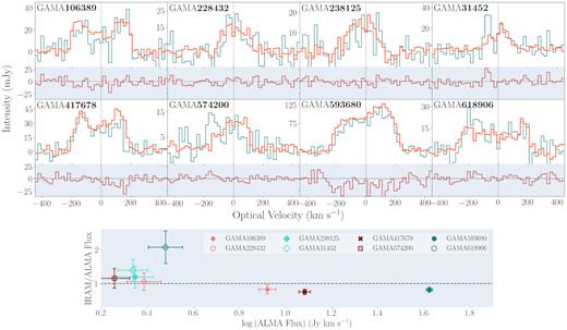
Top: Comparison of IRAM (teal) and ALMA (orange) CO(1→0) spectra for outflow-type galaxies in both observation samples. The IRAM–ALMA flux difference is shown below each plot. All galaxies in the figure are confirmed by the SAMI Galaxy Survey as harbouring galactic-scale outflows of ionized gas. The ALMA and IRAM spectra have been re-binned to a common spectral resolution of |$20\rm \ km~s^{-1}$|. Bottom: Comparison of the integrated CO(1→0) fluxes in the IRAM and ALMA objects with a linear 1:1 trend.
To verify that the ALMA maps are not missing any extended flux, we compare in Fig. 2 the integrated IRAM-30-m and ALMA CO(1→0) spectra for the eight galaxies that the samples have in common for which we have positive CO(1→0) detection. The spectra are re-binned to the same spectral resolution using the spectres package (Carnall 2017). There is a good agreement between the emission profiles measured with ALMA and IRAM, showing that ALMA has not resolved out significant amounts of flux. For 3 of the 16 galaxies (one outflow type and two controls) observed with ALMA, we do not detect CO(1→0) emission (i.e. S/N<3).
The total integrated flux is measured by numerically integrating each global ALMA CO(1→0) emission profile, where we define channels with signal detection as those with a flux above 3 standard deviations (3σ) of the noise in a line-free region. The uncertainty on this integrated flux is calculated as |$\sigma _{\rm err} = \rm 3 \sqrt{N}\ \sigma \ dv$|, where |$\rm N$| is the number of channels with signal >3σ and |$\rm dv$| is the channel width in km s−1. The global |$\rm L_{\rm CO}$| is calculated as explained in Section 2.1, with values presented in Table 2. As detailed in Section 2.1, we use the variable conversion factor derived by Accurso et al. (2017). This is done to account for the range of stellar mass (|$\rm M_*$|) and metallicity values in our ALMA outflow-type objects (see Fig. 3). Again, we use magphys |$\rm M_*$| and SFR estimates and emission line ratios from 3-arcsec apertures centred on our objects from SAMI to estimate the metallicity by the Pettini & Pagel (2004) calibration. These measurements and the values of variable αCO for each object are given in Table 1.
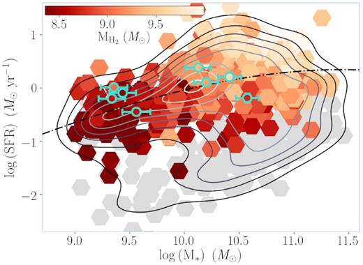
ALMA outflow-type objects plotted in the SFR – stellar mass (|$\rm M_{\rm *}$|) plane. Pale turquoise circles indicate an object identified as an outflow-type by SAMI (for which we have positive CO(1→0) detection). The xCOLD GASS catalogue is also given for comparison (red hexagons). The observed and catalogue objects are shaded by their molecular gas mass (|$\rm M_{\rm H_2}$|). Grey hexagons represent the objects in the xCOLD GASS catalogue with no CO(1→0) detection. The grey contours depict density levels in the xCOLD GASS catalogue and the black dashed line is the main-sequence trend as calculated by Saintonge et al. (2016).
Total CO(1→0) luminosities and |$\rm H_2$| molecular gas fractions for ALMA outflow-type objectsa.
| GAMA ID | S/NCOb | Flag b | σCO (|$\rm km~s^{-1}$|) b | |$\rm S_{\rm CO}$| (Jy km s−1) b | |$\rm z_{\rm CO}$| b | |$L^{\prime }_{\rm CO10}$| (|$10^8 \ \rm K \ km~s^{-1}\ {pc}^2$|) b | log (|$\rm M_{H_2} / M_*$|) b |
|---|---|---|---|---|---|---|---|
| 106389 | 33 | 1 | 169 | 8.33 ± 0.73 | 0.04012 | 6.13 ± 0.57 | −0.92 ± 0.20 |
| 228432 | 15 | 1 | 83 | 2.43 ± 0.46 | 0.02984 | 0.98 ± 0.19 | −0.34 ± 0.22 |
| 238125 | 14 | 1 | 77 | 2.23 ± 0.44 | 0.02581 | 0.68 ± 0.14 | −0.94 ± 0.23 |
| 31452 | 19 | 1 | 59 | 2.18 ± 0.35 | 0.02029 | 0.40 ± 0.08 | −1.08 ± 0.22 |
| 417678* | 53 | 1 | 140 | 12.09 ± 0.70 | 0.03946 | 8.63 ± 0.59 | −0.75 ± 0.20 |
| 567624 | <3 | 2 | – | – | – | – | – |
| 574200 | 18 | 1 | 69 | 1.81 ± 0.30 | 0.02867 | 0.67 ± 0.12 | −0.71 ± 0.22 |
| 593680 | 100 | 1 | 165 | 42.04 ± 1.40 | 0.03003 | 17.24 ± 1.16 | −0.71 ± 0.20 |
| 618906* | 10 | 1 | 184 | 3.02 ± 0.56 | 0.05648 | 4.45 ± 0.83 | −1.85 ± 0.21 |
| 239376 | <3 | 2 | – | – | – | – | – |
| 348116*⋆ | 23 | 1 | 196 | 8.85 ± 1.06 | 0.05036 | 10.34 ± 1.26 | −0.99 ± 0.20 |
| 496966* | 12 | 1 | 159 | 3.82 ± 0.70 | 0.05413 | 5.17 ± 0.95 | −1.24 ± 0.21 |
| 570227*⋆ | 27 | 1 | 208 | 8.45 ± 0.91 | 0.04332 | 7.30 ± 0.81 | −1.15 ± 0.20 |
| 618935 | 4 | 1 | 70 | 0.57 ± 0.21 | 0.03436 | 0.31 ± 0.12 | −1.46 ± 0.26 |
| 619098 | <3 | 2 | – | – | – | – | – |
| 623679* | 10 | 1 | 106 | 2.75 ± 0.62 | 0.05635 | 4.04 ± 0.92 | −1.07 ± 0.22 |
aObjects are divided by a horizontal line into outflow-type objects (above line) and control (i.e. non-outflow type) objects (below line).
bIf flag = 2, |$\rm {S/N}_{CO}$| < 3 (with adopted velocity range of 300 |$\rm km~s^{-1}$|) for the observation and we do not detect CO(1→0).
*Marked objects are from ALFALFA. For the unmarked galaxies, we have SAMI-H i data.
⋆Marked objects may be AGN-contaminated.
Total CO(1→0) luminosities and |$\rm H_2$| molecular gas fractions for IRAM positive-detection objectsa.
| GAMA ID | |$\rm {{S/N}_{CO}}^{b}$| | Flag b | σCO (|$\rm km~s^{-1}$|) b | |$\rm S_{\rm CO}$| (Jy km s−1) b | |$\rm z_{\rm CO}$| b | |$L^{\prime }_{\rm CO10}$| (|$10^8 \ \rm K \ km~s^{-1}\ {pc}^2$|) b | log (|$\rm M_{H_2} / M_*$|) b |
|---|---|---|---|---|---|---|---|
| 106389 | 10 | 1 | 169 | 6.90 ± 0.86 | 0.04015 | 5.18 ± 0.61 | −0.99 ± 0.17 |
| 209807* | 18 | 1 | 140 | 14.22 ± 1.39 | 0.05380 | 19.40 ± 1.81 | −1.12 ± 0.17 |
| 228432 | 8 | 1 | 37 | 2.57 ± 0.40 | 0.02979 | 1.06 ± 0.15 | −0.31 ± 0.18 |
| 238125 | 6 | 1 | 90 | 2.65 ± 0.50 | 0.02593 | 0.82 ± 0.14 | −0.86 ± 0.18 |
| 239249 | <3 | 2 | – | – | – | – | – |
| 31452 | 7 | 1 | 72 | 3.02 ± 0.51 | 0.02026 | 0.57 ± 0.10 | −0.93 ± 0.18 |
| 376121* | 8 | 1 | 188 | 4.28 ± 0.61 | 0.05148 | 5.33 ± 0.77 | −1.62 ± 0.17 |
| 383259* | 81 | 1 | 62 | 24.06 ± 1.95 | 0.05709 | 37.02 ± 3.00 | −0.85 ± 0.17 |
| 417678* | 23 | 1 | 137 | 9.12 ± 0.83 | 0.03950 | 6.63 ± 0.60 | −0.86 ± 0.17 |
| 486834* | <3 | 2 | – | – | – | – | – |
| 567624 | <3 | 2 | – | – | – | – | – |
| 574200 | 6 | 1 | 87 | 2.09 ± 0.39 | 0.02834 | 0.79 ± 0.14 | −0.63 ± 0.18 |
| 593680 | 35 | 1 | 170 | 34.26 ± 2.91 | 0.03007 | 14.33 ± 1.22 | −0.79 ± 0.17 |
| 618220* | 7 | 1 | 122 | 2.60 ± 0.44 | 0.05335 | 3.47 ± 0.58 | −1.49 ± 0.18 |
| 618906* | 9 | 1 | 181 | 6.24 ± 0.86 | 0.05653 | 9.38 ± 1.29 | −1.52 ± 0.17 |
| 209698* | 10 | 1 | 84 | 4.88 ± 0.62 | 0.02828 | 1.85 ± 0.22 | −1.26 ± 0.17 |
| 209743 | 10 | 1 | 109 | 5.05 ± 0.66 | 0.04056 | 3.88 ± 0.51 | −1.15 ± 0.17 |
| 279818 | 6 | 1 | 19 | 1.14 ± 0.22 | 0.02720 | 0.39 ± 0.08 | −1.29 ± 0.18 |
| 322910 | 13 | 1 | 20 | 2.51 ± 0.28 | 0.03093 | 1.12 ± 0.13 | −1.24 ± 0.17 |
| 346839* | <3 | 2 | – | – | – | – | – |
| 371976* | <3 | 2 | – | – | – | – | – |
| 41144 | 22 | 1 | 127 | 20.28 ± 1.87 | 0.02967 | 8.28 ± 0.76 | −1.00 ± 0.17 |
| log 517302 | 6 | 1 | 53 | 1.97 ± 0.38 | 0.02873 | 0.75 ± 0.15 | −2.00 ± 0.18 |
| 534753 | 20 | 1 | 96 | 17.76 ± 1.68 | 0.02863 | 6.79 ± 0.64 | −1.20 ± 0.17 |
| 570206* | <3 | 2 | – | – | – | – | – |
| 618151* | <3 | 2 | – | – | – | – | – |
| 620034 | 9 | 1 | 134 | 4.90 ± 0.66 | 0.04277 | 4.17 ± 0.56 | −1.12 ± 0.17 |
| 91996* | <3 | 2 | – | – | – | – | – |
a Objects are divided by a horizontal line into outflow-type objects (above line) and miscellaneous peculiar objects (below line).
b If flag = 2, |$\rm {S/N}_{CO}$| < 3 (with adopted velocity range of 300 |$\rm km~s^{-1}$|) for the observation and we do not detect CO(1→0).
*Marked objects are from ALFALFA. For the unmarked galaxies, we have SAMI-H i data.
3 RESULTS
The results of this paper are divided into two parts: Section 3.1 for our integrated results and Section 3.2 for our spatially resolved data. Due to contamination of our ALMA control sample by AGN and CO(1→0) non-detections, there are only three viable control objects. We compensate for this by including additional suitable control objects where possible in both our integrated and resolved analyses to create a more robust comparative sample for our outflow-type objects. In Section 3.1, we use a control sample derived solely from xCOLD GASS (referred to as the ‘xCOLD GASS controls’) for the interpretation of the global/integrated results (i.e. we do not include the original, viable ALMA controls).
For the resolved analysis in Section 3.2, we use additional spatially resolved data to supplement the three viable control objects we have from ALMA. Further CO(1→0) emission maps are not available for additional control galaxies, but we do extract extra controls from the SAMI sample (which we refer to as the ‘SAMI controls’) to aid analysis and validate the ALMA control sample. For any examination of our resolved CO(1→0) maps, we use only the three original controls from ALMA (referred to as the ‘ALMA controls’). The exact procedures for extracting supplemental controls from xCOLD GASS and SAMI will be detailed further in Sections 3.1 and 3.2.
3.1 Global molecular gas contents
The results of our integrated analysis are reported in Figs 3–6. We extract additional global properties for our objects (e.g. NUV − r) from the Galaxy And Mass Assembly (GAMA) DR2/DR3 catalogue (Liske et al. 2015; Baldry et al. 2018) with their respective uncertainties to supplement the interpretation of our results.
In our integrated analysis, we have replaced our observed ALMA control sample with objects derived from the xCOLD GASS catalogue. To compile a viable control sample, we identify the objects from xCOLD GASS with SFR and |$\rm M_*$| values within a |$0.3 \ \rm dex$| box centred on each galaxy within the ALMA outflow-type sample (see Fig. 3). We use magphys SFR and |$\rm M_*$| estimates for our outflow types, which are a sound comparison with xCOLD GASS estimators (Saintonge et al. 2018). Furthermore, we discount potential objects classed as AGN hosting based on the BPT diagnostic (Baldwin, Phillips & Terlevich 1981) and limit the objects’ inclination to i > 50°. For xCOLD GASS control objects with undetected CO(1→0), we use the 3σ upper limit for their molecular gas mass. From all the xCOLD GASS galaxies identified as prospective controls for each ALMA outflow-type galaxy, we extract |$80 {{\ \rm per\ cent}}$| at random (i.e. 0.8 × n objects, where n is the number of xCOLD GASS control objects identified for each galaxy). The median values of |$\rm M_*$|, SFR, |$\rm M_{H_2}$|, and NUV − r are used for the xCOLD GASS control object properties and their uncertainties (where the error on the median is estimated as 0.67 × 1σ). Given that the outflow-type galaxies identified by SAMI (and defined by Ho et al. 2016) are exceedingly rare in the redshift range spanned by xCOLD GASS, the probability of these xCOLD GASS controls also being ‘outflow types’ is statistically insignificant. The controls assembled from xCOLD GASS are given as the control sample alongside the ALMA outflow types in Figs 4–6.
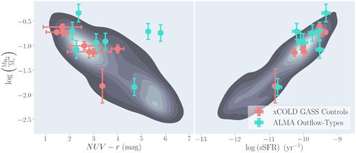
Molecular hydrogen mass (|$\rm M_{\rm H_2}$|) against both the NUV − r colour index (left-hand panel) and specific SFR (sSFR, right-hand panel) for the ALMA outflow-type sample with positive CO(1→0)-detection (turquoise) and averaged xCOLD GASS controls (red, see text) plotted alongside the xCOLD GASS catalogue (grey density contours).
![Comparison of molecular gas fractions ($f_{\rm M_{H_2}} = \rm M_{\rm H_2} / \rm M_{*}$) in ALMA outflow-type and xCOLD GASS-derived control galaxies (see text). The figure depicts the ‘swing’ of the difference in molecular gas fractions $\Delta f_{\rm M_{H_2}} = f_{\rm M_{H_2}, outflow} - f_{\rm M_{H_2}, control}$, with each inset disc representing one of the eight ALMA outflow-type galaxies [with positive CO(1→0) detection] and its corresponding xCOLD GASS control object. $\Delta f_{\rm M_{H_2}}$ is given by the position of the interface between blue and red regions (0.67 × 1σ uncertainties are also illustrated by the grey shaded areas). The ‘swing’ is given by the relative sizes of the blue (outflow-type) and red (control) regions. The uncertainty on the ‘swing’ is given by the shaded areas. The objects are ordered by their sSFR; the object with the highest sSFR value is the innermost ring and the object with the lowest is the outermost.](https://oup.silverchair-cdn.com/oup/backfile/Content_public/Journal/mnras/500/3/10.1093_mnras_staa3512/1/m_staa3512fig5.jpeg?Expires=1750203888&Signature=x0fUcgfbTBNgaJAQxmYNJ2MocnoW1ic6GcSrdJiO20lQThbkjTNefYEq08tlkvcV2TG60AHzUxJYctNI1wXnaf69uJoqXGmt8sFV~mF37TnGl9hWf4HRqHxuNCyny4~I~bC~KGg6xLHlMRsQRwiWKvCDgmMQArjlDspXkyXj8y6PxhzVjJpaMYorHWZHGYD7Waft9tEak2OCnkv~LDRZNx4y6A0HAqrGZ73g9S-MPdN-844~W-N-orlCUHx~kYGF4ikYbDq1vA~zfXyBirtvOPX2xDoUTxqIJwlbyPW2diN05-uDV3zCHla0wGlLHh5ZI4Wmc4PPBn7Jcz91U~bhfg__&Key-Pair-Id=APKAIE5G5CRDK6RD3PGA)
Comparison of molecular gas fractions (|$f_{\rm M_{H_2}} = \rm M_{\rm H_2} / \rm M_{*}$|) in ALMA outflow-type and xCOLD GASS-derived control galaxies (see text). The figure depicts the ‘swing’ of the difference in molecular gas fractions |$\Delta f_{\rm M_{H_2}} = f_{\rm M_{H_2}, outflow} - f_{\rm M_{H_2}, control}$|, with each inset disc representing one of the eight ALMA outflow-type galaxies [with positive CO(1→0) detection] and its corresponding xCOLD GASS control object. |$\Delta f_{\rm M_{H_2}}$| is given by the position of the interface between blue and red regions (0.67 × 1σ uncertainties are also illustrated by the grey shaded areas). The ‘swing’ is given by the relative sizes of the blue (outflow-type) and red (control) regions. The uncertainty on the ‘swing’ is given by the shaded areas. The objects are ordered by their sSFR; the object with the highest sSFR value is the innermost ring and the object with the lowest is the outermost.
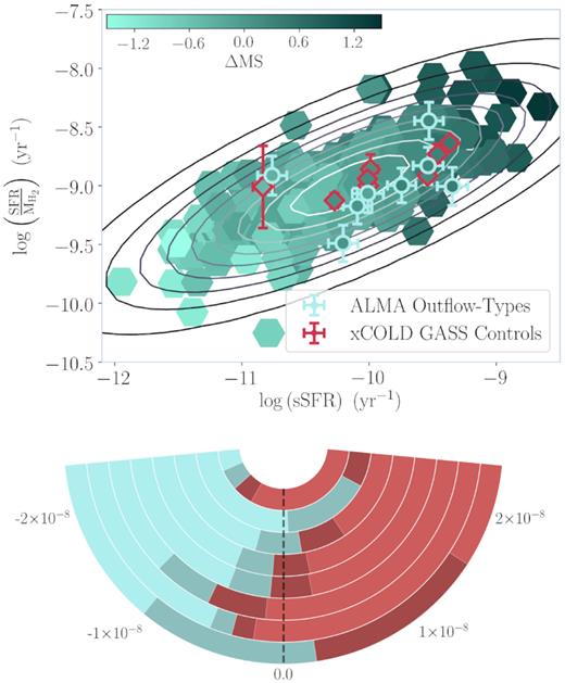
Top: ALMA outflow-type galaxies (light turquoise circles) and xCOLD GASS-derived controls (red diamonds) plotted with star-formation efficiency (|$\rm SFR/M_{\rm H_2}$|) against specific star-formation rate (sSFR). The xCOLD GASS catalogue is also depicted for comparison (green hexagons). The outflow-type, xCOLD GASS control and catalogue objects are shaded by the value |$\Delta \rm MS$|, which indicates the objects’ vertical displacement from the main-sequence trend in the SFR – |$\rm M_*$| plane as determined by Saintonge et al. (2016). The grey contours represent density levels in the xCOLD GASS catalogue. Bottom: ‘Swing’ plot depicting the quantity |$\Delta \rm SFE = SFE_{\rm outflow}-SFE_{\rm control}$|. The ring structure is equivalent to that used in Fig. 5 (i.e. ordering by the objects’ sSFR values); the turquoise represents the outflow types and the red the xCOLD GASS controls. The shaded areas represent the 0.67 × 1σ uncertainties.
The integrated properties of the outflow-type galaxies in our ALMA sample are given in Figs 3, 4, and 6 alongside the xCOLD GASS catalogue. The plots in Fig. 4 suggest little difference between the global properties of the ALMA outflow types and xCOLD GASS controls in terms of their sSFR and gas fractions. The similarity of both samples in these diagnostic figures implies that they do not contain fundamentally different galaxy types (see Section 4). We will analyse this further in Figs 5 and 6.
In Fig. 5, we use a novel ‘swing’ plot to assess the difference in molecular gas fractions between the ALMA outflow types and xCOLD GASS controls. The plot visualizes the quantity |$\Delta f_{\rm M_{H_2}} = f_{\rm M_{H_2}, outflow} - f_{\rm M_{H_2}, control}$| (i.e. the difference in molecular gas fraction between outflow-type |$f_{\rm M_{H_2}, outflow}$| and xCOLD GASS control |$f_{\rm M_{H_2}, control}$| galaxies), where each ring represents one of the eight ALMA outflow-xCOLD GASS control galaxy pairs. A positive ‘swing’ (i.e. the interface between blue and red regions has a positive angular value) indicates that the outflow type in the pair has the larger gas fraction compared to its xCOLD GASS control. Otherwise, a negative ‘swing’ indicates that the xCOLD GASS control possesses the higher gas fraction. The median ‘swing’ position is 0.05 ± 0.04, meaning the outflow types are only marginally more gas-rich compared to their control counterparts. This implies that outflow-type and our xCOLD GASS control galaxies have roughly equivalent reservoirs of material for further star-formation with respect to the stars they have already created.
Theory predicts that galaxies launching galactic-scale outflows possess lower gas fractions than galaxies without such violent outflows, due to their intense wind driving out reservoirs of cold molecular gas. However, our sample appears to contradict this conjecture. In order to scrutinize this behaviour, we derive the star-formation efficiency (SFE) for each outflow-type galaxy and xCOLD GASS control (see Fig. 6). We define this quantity as |$\rm SFR/\rm M_{H_2}$|, which has a positive correlation with specific star-formation rate (sSFR). The lower plot in Fig. 6 is a ‘swing’ plot for the quantity |$\Delta \rm SFE = \rm SFE_{\rm outflow} - \rm SFE_{\rm control}$|. Much as in Fig. 5, a positive value indicates that the outflow type in the outflow-control pair has the greater SFE and vice versa. We find no statistically significant average ‘swing’ across the galaxy pairs in this analysis (a median position of |$(0.006 \pm 0.03) \times 10^{-8}\,\rm yr^{-1}$|). Our outflow-type galaxies, therefore, do not appear to have a star-formation process that is globally more efficient than our xCOLD GASS control sample. We will consider the physical implications of these findings in Section 4.
We note in our outflow-type sample some anomalies in the physical appearance of GAMA31452 in the HSC optical images in Appendix A (visually, the arms are warped and show clear signs of major disruption). It is included in our sample due to the small sample size, but it may contribute to some level of contamination.
3.2 Spatially resolved observations
We extract spatially resolved information from our ALMA data cubes in the first instance by constructing moment maps (i.e. by collapsing the cubes over the respective moment axes). Moment maps are extracted using our own subroutines over a tight spatial box (∼22 arcsec × 22 arcsec) and trimmed channel range (∼45–50 channels) around the signal to minimize noise. We derive the zeroth, first, and second moment maps, representing 2D spatial maps of the intensity, velocity, and velocity dispersion of the gas, respectively. In order to adequately cut any extra-planar emission from the cubes, we initially smooth the data cubes both spectrally and spatially with a 2D Gaussian kernel using the Gaussian2DKernel and convolve sub-routines within the astropy.convolution package (Astropy Collaboration 2013, 2018). Spectrally, we smooth by a factor of 4 and spatially, we smooth by a factor of 1.5. From this smoothed cube, we create a mask by setting all values below 3σ of the noise level in the smoothed cube to zero in the original, un-smoothed cube. The final maps are presented in their entirety in Appendix B.
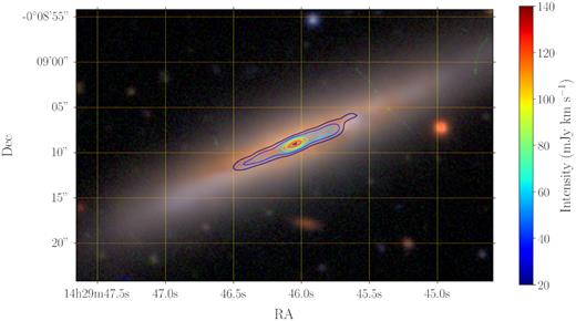
Zeroth moment map for GAMA593680 illustrated by colour-coded contours, drawn over an optical HSC (Hyper Suprime-Cam Subaru Strategic Program; Aihara et al. 2019) image (using bands g, r, and i) to allow a visual comparison of the extent of the CO(1→0) gas. The horizontal and vertical axes represent the RA and Dec directions, respectively.
Position-velocity diagrams (PVDs) were also extracted from the masked cubes to aid analysis of our objects. We produce PVDs by rotating the CO(1→0) by the position angle of the object (obtained from SAMI Galaxy Survey catalogues), so the galactic plane is parallel with the y-axis of the spaxel maps. A slit is then defined in the spatial plane that extends over the kinematic major axis of the CO(1→0) emission. The slit width is determined adaptively by the size of slit required to contain 95 per cent of the CO(1→0) emission for each object. We then collapse the cubes in the spatial direction perpendicular to the galactic plane to produce an image in offset – velocity space. We give examples of the output of this procedure in Fig. 8, where we show PVDs of GAMA593680, GAMA106389, and GAMA417678 (using slit widths of 1.6 arcsec, 2.4 arcsec, and 2.0 arcsec, respectively). PVDs for our full ALMA sample are given in Appendix C.
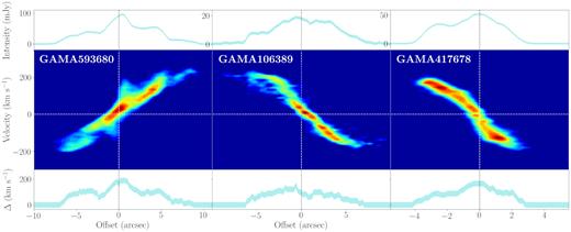
From left to right: PVDs of GAMA593680, GAMA106389, and GAMA417678 with offset on the horizontal axis in arcseconds and optical velocity (km s−1) on the vertical axis with respect to the objects’ redshift velocity. In each instance, the profile plotted above the PVD is the intensity as a function of offset (i.e. the profile obtained by collapsing over the velocity axis). The uncertainty is assumed as 3 standard deviations of the collapsed data (depicted as the width of the line in the profile). The bottom plots give the width in the velocity direction of the emission (Δ). The width is defined as where the emission is above 2 standard deviations of the noise and the uncertainty is given by the velocity change over a pixel width. Using a simple model, GAMA593680 (far left) is interpreted as the emission resulting from two, concentric Gaussian rings. GAMA106389 (centre) is best described by a Sersic/exponential profile. GAMA417678 is not in equilibrium and, therefore, has no simple model.
In every instance, we find the emission of CO(1→0) to be largely centralized in a thin disc. Furthermore, in the second moment maps in Appendix B, we observe that the beam-smeared velocity dispersion does not exceed ≈80 km s−1 in the cases of the outflow-type galaxies, far below that typically measured along lines of sight towards molecular outflows.
Fig. 8 also demonstrates the gas disc properties and kinematics that we observe in our sample. From a simple visual analysis, we identify three different gas structures from the PVDs and intensity profiles: GAMA593680 (left-hand panel) possesses no traits of the classic Sersic/exponential surface brightness profile and, by eye, would appear to be suggestive of two concentric rings, reminiscent of those caused by bar resonances. The apparent asymmetry may be due to a clumpy spiral structure within the galaxy and displays classic signatures of a central bar; GAMA106389 (centre panel) is more prosaic, having a structure and surface brightness profile suggestive of a Sersic/exponential disc at the centre of the galaxy (there is suggestion of a ‘hole’ towards the centre of the distribution); GAMA417678 (right-hand panel) appears far more extended on one side of its kinematic centre than the other, which may be indicative of a disturbed system. If the gas disc is not in equilibrium, it may be difficult to model accurately.
As previously discussed, in addition to the three viable ALMA control galaxies (GAMA496966, GAMA618935, and GAMA623679), additional control galaxies were selected from the SAMI Galaxy Survey data base to strengthen the results of our resolved analysis. In Fig. 9, we demonstrate how our ALMA outflow-type objects fall into roughly two groups based on their stellar masses; low-|$\rm M_*$| (log M* < 10) and high-|$\rm M_*$| (log M* > 10). In order to take account of this apparent dichotomy in our outflow-type objects, we draw two independent control samples from SAMI based on the location of the ALMA low-|$\rm M_*$| and high-|$\rm M_*$| outflow types in the SFR-|$\rm M_*$| plane (again using magphys estimates). We select the SAMI objects for our additional control samples based on two regions surrounding the aforementioned low-|$\rm M_*$| and high-|$\rm M_*$| ALMA outflow-type objects, as depicted in Fig. 9. The area of both regions in the SFR-|$\rm M_*$| plane is 0.6 × 0.7 dex centred on the mean position of the low-|$\rm M_*$| and high-|$\rm M_*$| outflow types, respectively (both regions have the same area, where the region size approximates the maximum scatter in |$\rm M_*$| and SFR). The possible redshifts and ellipticities of the SAMI controls are limited to below the maximum values in the outflow-type sample (the final selection is given in Fig. 9). We also discount any AGN-contaminated objects by excluding those with [N ii]/Hα and [O iii]/Hβ ratios indicative of AGN excitation in the BPT diagram.
![Selection of additional SAMI control sample in the SFR – $\rm M_*$ plane. Turquoise markers indicate ALMA outflow-type objects, which broadly fall into lower and higher stellar mass regions of the SFR – $\rm M_*$ plane [i.e. $\log (\rm M_*) \lt 10$ and $\log (\rm M_*) \gt 10$]. Two control samples are drawn from the SAMI Galaxy Survey from the regions shaded in grey (which cover 0.7 × 0.6 dex in the SFR – $\rm M_*$ plane), centred on the mean position of the low-$\rm M_*$ and high-$\rm M_*$ outflow-type objects, respectively. The objects selected from SAMI Galaxy Survey are given by the red and dark blue markers in the low- and high-$\rm M_*$ regions, respectively. The grey contours depict density levels in the xCOLD GASS catalogue and the black dashed line is the main-sequence trend as calculated by Saintonge et al. (2016).](https://oup.silverchair-cdn.com/oup/backfile/Content_public/Journal/mnras/500/3/10.1093_mnras_staa3512/1/m_staa3512fig9.jpeg?Expires=1750203888&Signature=pwh9qX~hdvO~bRsagJ5g7h3scbrcax0aSxT1-FJRnFVbR1-P4okQIJdPw26hXtqksc71x5wn4jRaLlV~XU6Zqlewud1tGpI6nN4crwLbYtmrJZyhDax-Xu6eg-t6O17sl0Qm3U70MIWm-ZVc7S7XL0Zwqzp8~53qj9TrwS96AQ1JnwhsVmyz8sM7O4SZnCrdV68OpPvwWcf~tfqaCYjzSYD4B43-y2HjaZ7e9L8gTrMdomJunylnFIILNgfMRaKQt9hi9YC~ZL8ERe6DvyZyABwov93WBDoAo8LyTtmmC7NouF6rQXLEcFG45ZsV6BWR2wYeVULIsg79bltgxW~vFQ__&Key-Pair-Id=APKAIE5G5CRDK6RD3PGA)
Selection of additional SAMI control sample in the SFR – |$\rm M_*$| plane. Turquoise markers indicate ALMA outflow-type objects, which broadly fall into lower and higher stellar mass regions of the SFR – |$\rm M_*$| plane [i.e. |$\log (\rm M_*) \lt 10$| and |$\log (\rm M_*) \gt 10$|]. Two control samples are drawn from the SAMI Galaxy Survey from the regions shaded in grey (which cover 0.7 × 0.6 dex in the SFR – |$\rm M_*$| plane), centred on the mean position of the low-|$\rm M_*$| and high-|$\rm M_*$| outflow-type objects, respectively. The objects selected from SAMI Galaxy Survey are given by the red and dark blue markers in the low- and high-|$\rm M_*$| regions, respectively. The grey contours depict density levels in the xCOLD GASS catalogue and the black dashed line is the main-sequence trend as calculated by Saintonge et al. (2016).
Fig. 10 bins ΣSFR maps for our outflow type, ALMA control, and SAMI control samples by spaxel values. Given the diversity of global properties we find in Fig. 9, in Fig. 10, we give the spaxel distribution for each ALMA outflow-type object in separate panels instead an averaged sample over the group to avoid domination of individual objects in a statistically small sample or the loss of information by assuming that these objects will have similar SFR distributions. The low-|$\rm M_*$| and high-|$\rm M_*$| outflow-type objects are on the bottom and top rows of Fig. 10, respectively, and ordered on each row by specific SFR (sSFR) from highest to lowest from left to right. In each panel, we also plot the averaged histograms for both the ALMA and SAMI controls (i.e. histograms including spaxels from every object in those samples), which are scaled by the number of objects in the respective groups in order to allow visual comparison.
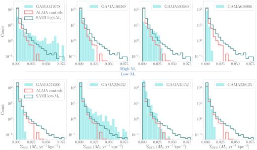
Histograms of SFR density per spaxel (ΣSFR) for each ALMA outflow-type object (turquoise bars). The objects are separated into two rows according to their stellar masses (high-|$\rm M_*$| and low-|$\rm M_*$|) as described in the text and ordered on each row by specific SFR (sSFR) from highest to lowest from left to right. The averaged ΣSFR distributions of the ALMA control sample (red step bars) and additional SAMI control samples (low- and high-|$\rm M_*$|, teal step bars) are also given in each panel. We re-bin our spaxel areas to the dispersion of the SAMI PSF (σPSF), which corresponds to a physical scale of |$\approx 1 \rm \ kpc$|.
We do not find consistent evidence of higher ΣSFR in our ALMA outflow-type objects Fig. 10 in relation to the ALMA control sample or additional SAMI controls. In the instances of GAMA417678 and GAMA228132 (a high-|$\rm M_*$| and a low-|$\rm M_*$| object, respectively), there does appear to be a significant elevation in the dense spaxel tail of their ΣSFR distribution. However, the majority of the outflow types do not appear to possess higher ΣSFR spaxels compared to the distributions drawn from the ALMA and SAMI control samples.
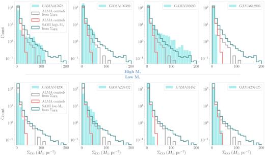
Histograms of molecular gas density per spaxel (ΣCO) for each ALMA outflow-type object (turquoise bars). The objects are separated into two rows according to their stellar masses (high-|$\rm M_*$| and low-|$\rm M_*$|) as described in the text and ordered on each row by specific SFR (sSFR) from highest to lowest from left to right. For comparison, the averaged ΣCO distribution of the ALMA control sample (red step bars) is given in each panel. Using the ΣSFR – |$\Sigma _{\rm CO, H_2}$| relation determined by Leroy et al. (2013), we also give the transformed ALMA control group and SAMI high-|$\rm M_*$|/low-|$\rm M_*$| from the ΣSFR spaxel distribution in Fig. 10 (teal step bars). We re-bin our spaxel areas to the dispersion of the SAMI PSF (σPSF), which corresponds to a physical scale of |$\approx 1 \rm \ kpc$|.
Again, we do not find a consistent elevation of ΣCO in our ALMA outflow-type objects with regard to the ALMA control sample or SAMI control samples. However, as is also the case in Fig. 10, we do find evidence of higher ΣCO spaxels compared to the control samples in a portion of our outflow-type objects. Low-|$\rm M_*$| object GAMA228432 and high-|$\rm M_*$| objects GAMA106389, GAMA417678, and GAMA593680 possess an enhancement of ΣCO spaxels with respect to the ALMA control sample (where both GAMA228432 and GAMA417678 were also noted in Fig. 10 to have elevated ΣSFR spaxels). Only GAMA593680, however, appears to possess significantly enhanced ΣCO relative to the SAMI control sample (transformed via equation [7]). It should be noted that this does not correspond with either of the objects observed to have ΣSFR enhancement in Fig. 10 (i.e. GAMA417678 and GAMA228432).
In Fig. 12, we assess the distribution of ΣSFR with respect to radius along the plane of the edge-on disc (where the radial positions of the spaxels are normalized by the objects’ effective radii, reff). In these bar plots, spaxels are binned by their distance from the centre of the galaxy (the centre defined by the RA and Dec coordinates drawn from the TilingCatv29 catalogue in the GAMA Survey, Driver et al. 2009; Baldry et al. 2010) in the direction along the plane (i.e. determined by the position angle given by the SersicCatAllv07 catalogue in the GAMA Survey, Kelvin et al. 2012). The sizes of the bars in Fig. 12 are determined by the SAMI resolution in kpc (approximated as the dispersion of a SAMI PSF of σPSF ≈ 2 arcsec at the most distant galaxy) divided by the median reff across our ALMA outflow types and ALMA controls. The mean spaxel value in each distance bin is then calculated to give the height of the bars (where the 3σ error is taken as the uncertainty). Again, we present the distribution for each outflow type individually and average together the objects in the comparative control groups. The layout of the panels in the figure is equivalent to those in Figs 10 and 11.
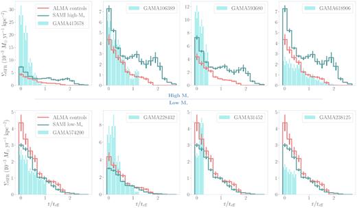
Bar plot depicting the average values of ΣSFR spaxels (scaled to the SAMI resolution) binned by their radial distance for each outflow-type object (turquoise bars) from the centre along the plane of the edge-on disc. In each panel, we also give the averaged radial profiles derived from our ALMA control group (red step bars) and additional control groups drawn from SAMI (teal step bars, see text). The radial distances of ΣSFR spaxels are normalized by the individual objects’ effective radii (reff) and the bars are binned at intervals of 1 kpc over the median reff of all objects in the outflow-type and ALMA control samples to approximate the width of SAMI PSF. The uncertainties represent 3 standard errors (3σ) in the mean spaxel value of each distance bin. The outflow-type objects are separated into high-|$\rm M_*$| and low-|$\rm M_*$| subgroups in the figure, with the radial distributions of the high-|$\rm M_*$| objects on the top row and the low-|$\rm M_*$| on the bottom row (presented with the SAMI high-|$\rm M_*$| and SAMI low-|$\rm M_*$| additional control groups, respectively). Each row is ordered by the objects’ specific SFR (sSFR) from highest to lowest from left to right.
In the ΣSFR radial distribution, we observe a greater degree of central concentration in our ALMA outflow-type objects with respect to the ALMA control and additional SAMI control samples. With the exception of GAMA618906, the ΣSFR radial distributions of our ALMA outflow-type objects are confined to their inner |$\lesssim 1.5 \rm \ r_{eff}$|. However, we do not see a consistent elevation in mean ΣSFR spaxel values with radius in the ALMA outflow types compared to the control distributions. With regard to the ALMA control and SAMI low-|$\rm M_*$| and high-|$\rm M_*$| control samples, we observe a greater similarity between the ALMA control radial distribution with that of the SAMI low-|$\rm M_*$| controls. The ALMA control sample comprised three objects, two of which are in the SAMI low-|$\rm M_*$| control sample, with the other lying outside, but between, the SAMI low-|$\rm M_*$| and high-|$\rm M_*$| regions in the SFR-|$\rm M_*$| plane. This may suggest that our ALMA control sample is more suitable as a control group for our low-|$\rm M_*$| outflow-type objects. The difference in the SAMI low-|$\rm M_*$| and high-|$\rm M_*$| radial profiles also supports our treating of these two groups in our outflow types in isolation. In comparison to the SAMI high-|$\rm M_*$| ΣSFR radial profile, all our high-|$\rm M_*$| outflow types have a more centralized distribution.
In Fig. 13, we plot the radial distribution of the |$\rm \Sigma _{CO}$| spaxels in our objects. The bar plot panels have the same format as Fig. 12 (i.e. bar width, panel order etc.). As in Fig. 11, we transform the radial ΣSFR distribution of the ALMA controls along with the SAMI low-|$\rm M_*$| and high-|$\rm M_*$| controls given in Fig. 12 into ΣCO using equation (7). We do this in order to validate our ALMA control sample, which, as in the ΣSFR radial distribution, is in good agreement with the SAMI low-|$\rm M_*$| ΣCO radial profile [the similarity between the ΣCO distribution derived from our ALMA control maps and that calculated using equation (7) from the ΣSFR distribution also validates our use of the conversion for our additional SAMI control samples].
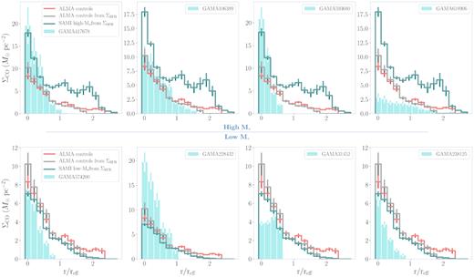
Bar plot depicting the average values of ΣCO spaxels (scaled to the SAMI resolution) binned by their radial distance for each outflow-type object (turquoise bars) from the centre along the plane of the edge-on disc. In each panel, we also give the averaged radial profiles derived from our ALMA control group (red step bars). The radial distances of ΣCO spaxels are normalized by the individual objects’ effective radii (reff) and the bars are binned at intervals of 1 kpc over the median reff of all objects in the outflow-type and ALMA control samples to approximate the width of SAMI PSF). The uncertainties represent 3 standard errors (3σ)in the mean spaxel value of each distance bin. The outflow-type objects are separated into high-|$\rm M_*$| and low-|$\rm M_*$| subgroups in the figure as in Fig. 12. Using the ΣSFR – |$\Sigma _{\rm CO, H_2}$| relation determined by Leroy et al. (2013), we also give the transformed ALMA control group and SAMI high-|$\rm M_*$|/low-|$\rm M_*$| from the ΣSFR radial profiles in Fig. 12.
Again we find a greater central concentration of ΣCO in our ALMA outflow-type objects in comparison to our ALMA and SAMI control samples. If we take the high-|$\rm M_*$| SAMI control group as the comparative controls for the ALMA high-|$\rm M_*$| outflow-type objects (i.e. the top row in Fig. 13), this centralization is particularly clear. For the majority of our outflow-type objects, the gas distribution lies in the inner |$\approx \rm \ r_{eff}$| of their respective discs, except for GAMA106389 and GAMA618906, which have distributions out to |$\approx \rm \ 2 r_{eff}$|. However, the two aforementioned objects still have gas distributions that are more centrally distributed with regard to the SAMI high-|$\rm M_*$| controls. The ΣCO distribution for our ALMA outflow-type objects, therefore, strongly resembles that of the ΣSFR profiles given in Fig. 12. Similarly, we do not find higher density gas spaxels with respect to radius consistently in our objects, which we also infer from Fig. 11.
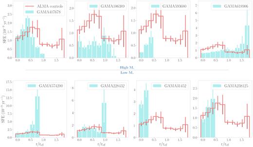
Bar plot depicting the average values of SFE spaxels (scaled to the SAMI resolution) binned by their radial distance for each outflow-type object (turquoise bars) from the centre along the plane of the edge-on disc. SFE spaxels are calculated from our ALMA CO(1→0) maps degraded to the SAMI resolution and SFR maps derived from SAMI Galaxy Survey data products (see text). In each panel, we also give the averaged radial profiles derived from our ALMA control group (red step bars). The radial distances of SFE spaxels are normalized by the individual objects’ effective radii (reff) and the bars are binned at intervals of 1 kpc over the median reff of all objects in the outflow-type and ALMA control samples to approximate the width of SAMI PSF. The uncertainties represent 3 standard errors (3σ) in the mean spaxel value of each distance bin. The outflow-type objects are separated into high-|$\rm M_*$| and low-|$\rm M_*$| subgroups in the figure as in Fig. 12.
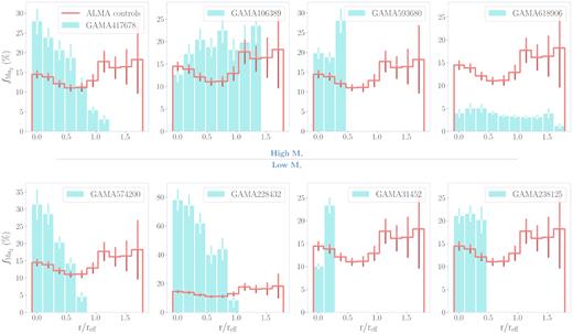
Bar plot depicting the average values of |$f_{\rm M_{H_2}}$| spaxels (scaled to the SAMI resolution) binned by their radial distance for each outflow-type object (turquoise bars) from the centre along the plane of the edge-on disc. |$f_{\rm M_{H_2}}$| spaxels are calculated from our ALMA CO(1→0) maps degraded to the SAMI resolution and stellar mass maps by Taylor et al. (2011). In each panel, we also give the averaged radial profiles derived from our ALMA control group (red step bars). The radial distances of |$f_{\rm M_{H_2}}$| spaxels are normalized by the individual objects’ effective radii (reff) and the bars are binned at intervals of 1 kpc over the median reff of all objects in the outflow-type and ALMA control samples to approximate the width of SAMI PSF. The uncertainties represent 3 standard errors (3σ) in the mean spaxel value of each distance bin. The outflow-type objects are separated into high-|$\rm M_*$| and low-|$\rm M_*$| subgroups in the figure as in Fig. 12.
To construct the SFE maps, we divide SFR and molecular gas mass map spaxels and produce Fig. 14 by the same method used to create the ΣSFR and ΣCO radial plots in Figs 12 and 13. The radial limit of the plot only extends to 2reff due to the lack of significant SFE spaxels in the outer regions of the objects. For our radial SFE profiles in Fig. 14, we use the ALMA controls as the control sample. We do not observe any consistent enhancement of SFE in our outflow-type objects with regard to the ALMA controls. From this, we could infer that we are not observing a more efficient process of star-formation in the outflow-type objects compared to that taking place in the ALMA controls.
Our |$\rm f_{M_{H_2}}$| maps require maps of stellar mass, which have been derived from pixel-matched ugriZYJ imaging from VST-KiDS and VISTA-VIKING. The imaging has been reprocessed by the GAMA survey (Driver & GAMA Team 2016) and re-projected to match the pixel scale of the SAMI cubes (0.5-arcsec pix−1). Stellar masses are calculated from the synthetic stellar population modelling of the per-pixel u-J SEDs, in a similar way to the GAMA stellar mass estimates (Taylor et al. 2011). We divide the molecular gas mass (again degraded to the SAMI resolution) and stellar mass spaxels and bin radially using the same method described for Fig. 14 to produce a radial distribution of |$\rm f_{M_{H_2}}$| for the ALMA outflow types and ALMA control sample. Similar to the radial profiles plotted for ΣSFR and ΣCO, we observe a more centralized radial distribution of |$\rm f_{M_{H_2}}$| in the outflow types compared to the flatter distribution in the ALMA controls. We also see higher values of |$\rm f_{M_{H_2}}$|, in particular but not exclusively, within the inner ≈0.5reff of the outflow types (again, with the exception of GAMA618906). This may suggest that our outflow types possess higher gas content relative to their stellar mass inside their innermost regions compared to the ALMA control group.
4 DISCUSSION
4.1 Equivalent outflow-control global gas content
Following Fig. 5, we observe no notable difference in global molecular gas fraction between our outflow-type sample and their xCOLD GASS control objects (see Section 3.1). This would appear to contradict expectations that galaxies with intense ionized outflows would be more gas-poor due to the entrainment of their molecular gas in the outflowing stellar wind. This result is also at odds with previous studies that have shown differences in gas content in galaxies harbouring intense ionized outflows and those that do not. However, we note the absence in this analysis of H i gas content in our outflow types and controls (as we do not have H i for all our ALMA outflow-type/control sample). It remains possible, therefore, that the samples contain different total amount of cold gas (defined as H i + |$\rm H_2$|). Roberts-Borsani et al. (2020) find indications of lower H i gas fractions in their outflow-type sample compared to their corresponding control group. This may suggest that the total cold gas fraction in our outflow-type sample may be depleted compared to the controls, while their molecular gas fractions are equivalent. Nevertheless, it is clear from this work that the outflow-type objects do not have a significantly different molecular fraction (i.e. |$\rm M_{\rm H_2}/M_{\odot }$|) compared to non-outflow-type galaxies with normal levels of star-formation. However, we must also consider that the gas potentially being expelled from our outflow types may not escape the objects and may instead fall back down to the disc (‘galactic fountain model’, Shapiro & Field 1976). Given the relatively low-velocity dispersion measurements we find in our ALMA moment maps (see Appendix B), it is unlikely that the gas possesses outflow velocities greater than circular velocity of the objects (i.e. |$\rm \sigma _{CO} \lt v_{circ}$|), meaning the gas would have insufficient energy to escape the gravitational well of the host galaxy (see Roberts-Borsani & Saintonge 2019). Any outflowing gas, therefore, may be recycled down as an inflow, meaning our integrated gas fraction values would not appear depleted by the presence of outflows in our objects. Differences in integrated gas fraction between our outflow types and control objects may require higher energy outflows than we observe in our ALMA outflow-type sample. However, it should be noted that our ALMA objects are highly inclined, meaning the |$\rm \sigma _{CO}$| values we measure are largely dominated by motions into/out of the plane of the discs. Outflows along the minor axes, therefore, would be difficult to detect in |$\rm \sigma _{CO}$|. As the gas we observe is contained within a thin disc, without significant CO(1→0) emission outside the plane, it would seem that these objects are not entraining large quantities of molecular gas.
In our resolved analysis in Section 3.2, Fig. 13 shows evidence that, despite the similarity in global gas content between our outflow-type and xCOLD GASS control galaxies, the spatial distribution of molecular gas is not equivalent when compared to the resolved ALMA and SAMI control samples. We find that our outflow-type objects possess more central gas distributions and a steeper decline of gas density with radius, with most harbouring their gas within their inner ≈reff. This is compared to the ALMA and SAMI control groups that have less central ΣCO distributions with a shallower radial decline. This is consistent with the idea that ΣSFR is the primary driver of outflows and that outflows are strongest in the central regions of galaxies (see Roberts-Borsani et al. 2020). However, as shown by Fig. 11, we do not find denser spaxels of ΣCO in our outflow types, nor a higher incidence of dense spaxels, with respect to the ALMA and SAMI control groups. Our radial distribution of molecular gas in Fig. 13, therefore, suggests that the densest regions of gas in our outflow types are located in the central regions of the objects, whereas in the ALMA and SAMI control samples, the dense regions are less centrally concentrated.
4.2 Centralized ΣSFR and ΣCO in outflow-type galaxies
Fig. 12 illustrates the difference in the distribution of ΣSFR with radius between our ALMA outflow types and our control samples. As previously noted, the outflow-type galaxies appear to possess more centrally distributed star-formation compared to the ALMA and SAMI controls, which display a comparatively shallow decline of ΣSFR with radius. One can infer from our findings that the star-formation in outflow-type galaxies occurs in a well-defined, central region, which could induce powerful stellar winds emanating from that central area. This result is in agreement with Roberts-Borsani et al. (2020), where ΣSFR is also found to extend out to ≈reff in their outflow-type objects. However, we note that we do not find evidence of a consistent elevation of ΣSFR spaxels in the outflow-type objects relative to the control samples. Currently, star-formation is the main mechanism theorized to drive supersonic turbulence within the ISM in low redshift galaxies (Mac Low & Klessen 2004). If this hypothesis holds, cold gas should be entrained by highly turbulent stellar winds within the central regions of our outflow-type galaxies, potentially expelling it along with large-scale outflows of ionized gas. Within this work, we do not find evidence of this either by detecting spatially extended emission in the zeroth moment maps (see Fig. 7) or by kinematic signatures in the PVDs (see Fig. 8). However, using stacking in extra-planar regions in future analyses may reveal the presence of CO gas entrained within the ionized gas ejections from our outflow-type objects.
Fig. 13 also implies a centralization of ΣCO spaxels in our outflow-type objects compared to the ALMA and SAMI controls. This is in agreement with analysis conducted by Schruba et al. (2011) on the CO(2→1) emission of local spiral galaxies within the IRAM HERACLES survey. They report a characteristic exponential decline of CO(2→1) emission in the central region of their galaxy sample with no sharp cutoff. Furthermore, Roberts-Borsani et al. (2020) find signatures of outflow activity, using the Na d λλ5889, 5895 Å neutral gas tracer, to be largely confined to the central ≈reff of their outflow-type objects from the MaNGA DR15 survey (Bundy et al. 2015). Outside this central region, they find a steep decline in mass outflow rates and loading factors, implying that outflow activity occurs almost exclusively in the centre of galaxies. The centralization of molecular gas in our outflow types, and those in other studies, suggests the existence of a mechanism driving gas inwards towards the inner ≈reff in these objects.
We also find in our resolved radial distribution a centralization of molecular gas fraction spaxels in our outflow-type objects compared to the ALMA control sample. The distribution of outflow-type and ALMA control gas fraction spaxels in Fig. 15 suggests that the outflow types have a central enhancement (within the inner |$\approx \rm 0.5 r_{eff}$|) of molecular gas relative to the stellar mass, unlike the ALMA controls. In Fig. 13, we do not observe a consistent elevation of central molecular gas content in the ALMA outflow types with respect to the ALMA control sample but do see a steeper decline with radius. The central enhancement of gas fraction must, therefore, be driven by a greater proportion of gas with respect to the stellar mass in the inner |$\approx \rm 0.5 r_{eff}$|. Fig. 15 further indicates that the gas distribution is more regular in the ALMA control group with regard to the stellar population and suggests that there is a greater supply of gas in their outer regions relative to the stellar mass. Furthermore, the similarity of the SFE radial profiles between our outflow-type and ALMA controls implies that there is not a more efficient mechanism operating within galaxies harbouring large-scale galactic outflows and that SFE is fairly uniform throughout their discs.
This enhanced central gas fraction, in combination with the evidence of intense ionized outflows, could be further evidence of a ‘galactic fountain’ scenario, where ejected molecular gas is falling back down to the disc (i.e. it is not escaping the gravitational well of the host galaxy). The molecular gas fraction in our outflow-type objects would, therefore, not be depleted by the existence of outflow activity. After falling back to the disc, a separate mechanism may then act to drive the gas inwards to the central regions of the outflow-type object (see Sections 4.2.1 and 4.2.2). In contrast to our findings concerning the molecular gas fraction, Roberts-Borsani et al. (2020) find evidence that the neutral gas fraction is depleted in the central regions of their outflow-type sample (where H i is measured through stacking of H i 21-cm observations). The combination of these results suggests that while molecular |$\rm H_2$| gas is driven towards the centre of outflow-type galaxies, H i is simultaneously being propelled towards their outer regions, perhaps tracing the ionized wind. Equally, H i that does fall inwards may be converted into |$\rm H_2$| in the centre of the objects due to high pressures in the central regions.
We can infer from our findings that a mechanism operates in the ALMA outflow types that is driving gas towards the centre of the objects and stripping their outer regions of the surrounding gas.
4.2.1 Bar-driven gas transport
The difference in distributions of ΣSFR and ΣCO between our outflow types and their respective control samples is likely indicative of a different mechanism governing the dynamics of gas within the two galaxy classifications. Jogee, Scoville & Kenney (2005) explore the ability of bars to re-distribute angular momentum in a galaxy, efficiently driving molecular gas into its central regions. Large asymmetric structures, such as bars, are capable of exerting immense torques on the surrounding gas, causing it to lose angular momentum and, consequently, fall inwards.
Fig. 8 illustrates, with three distinct examples, the wide variety in the morphology and kinematics of the gas discs within our ALMA objects. Jogee et al. (2005) also note this diversity of CO morphologies within their sample of barred galaxies. In particular, they suggest that an extended molecular gas distribution is indicative of the early stages of bar-driven inflows (meaning a large fraction of the circumnuclear gas is still along the large-scale stellar bar). By contrast, bar structures in a later stage of their evolution are typically found to hold their circumnuclear gas within the OILR (outer inner Lindblad resonance) of the bar. This gas is likely to exhibit principally circular motion as opposed to gas in a younger bar structures, which tends towards non-circular kinematics.
Unlike Jogee et al. (2005), Sheth et al. (2005) make the distinction that only early-type Hubble barred spirals (i.e. CO-bright galaxies) demonstrate the very disparate environment within the central 1–2 kpc compared to the outer regions. This difference between early-type and late-type barred spirals is typically attributed to the higher critical surface densities required for star-formation in early types, resulting from steeper rotation curves (Ho, Filippenko & Sargent 1997). Ho et al. (1997) predict, consequently, that early-type barred spirals will have higher central gas concentrations. Furthermore, they theorize that in order for these early-type spirals to maintain their high-density cores, they must have substantially higher mass inflow rates compared to late-type spirals. Our outflow-type objects may, therefore, be more consistent with late-type barred spirals, possessing a central symmetry sufficient to cause molecular gas to fall inwards but without the high gas densities and SFR observed in early-type spirals.
Future kinematical modelling should help elucidate the structure of these galaxies and whether they are consistent with the definition of Hubble late-type.
4.2.2 Interaction-driven gas transport
Galactic interactions are widely accepted to initialize widespread disc destabilization. Large-scale disruption of this kind is also commonly associated with the formation of asymmetric galactic features. These asymmetries established within the merging discs exert strong torques on the adjacent gas, causing it to fall inwards. This is supported by the work of Di Matteo et al. (2007), where the gas dynamics of merging galaxy pairs is modelled in detail. They simulate over 200 merging pairs and observe several key phases of gas contraction and expansion. The final stage of the merger involves a violent inflow of between |${\approx }50 \!-\! 80 {{\ \rm per\ cent}}$| of the total gas mass and is triggered by the rapid fluctuations in the galactic potential. This gas flows into the central kiloparsec of the merger and can be followed by an intense starburst (which persists for <600 Myr). However, Di Matteo et al. (2007) note that interacting pairs do not always lead to star-formation enhancement. Moreover, they find that high star-formation enhancement is an infrequent result in their simulations (compared to no, low, or moderate enhancement) and is associated with the shortest starburst duration times. This scenario is consonant with our results in this study. Furthermore, Di Matteo et al. (2007) also find relatively small differences between the global SFR values for interacting and non-interacting galaxies (also reported by Bloom et al. 2017), which supports the integrated analysis presented in Figs 4 and 6.
Again, in order to find evidence of interaction, detailed kinematic analysis is required. From initial observations, Fig. 8 appears to suggest that some of the kinematic profiles are indicative of disturbed gas structures. However, our moment maps and PVDs suggest settled, regular gas structures in many of our outflow-type objects. It may be, therefore, that our outflow-type sample comprised objects undergoing a variety of processes that drive molecular gas inwards and expel intense ionized winds.
4.3 Effect of time-scales
Throughout our resolved analysis in Section 3.2, we treat our ALMA outflow types individually due to the wide variety of global (e.g. metallicity and stellar mass) and resolved properties (i.e. some objects possess enhanced star-formation and gas density, while others do not) that we observe in the sample. As discussed previously, we also find a wide variety of kinematical structures in our outflow-type objects in Fig. 8. The diversity of these properties suggests that these objects are either a collection of unrelated galaxies, similar only in their shared proclivity to eject large amounts of ionized gas, or similar objects at different stages in their evolution. For example, in relation to the discussion in Section 4.2.2, it is possible that our outflow types are interacting galaxies but at different stages of their evolution. As detailed by Di Matteo et al. (2007), mergers enter phases of gas compression with short-lived, central starbursts and gas expansion with little star-forming activity and diffuse molecular gas distributions. If interaction is the driver of the molecular gas compression and large-scale outflows of ionized gas in our outflow-type objects, it is possible that our outflow types are at different stages in the compression–expansion cycle but all still experiencing large-scale ionized outflows. This would be supported by the indications of instability in the PVDs shown in Fig. 8. However, as previously noted, kinematical analysis is required to validate this possibility and whether the diversity of kinematical structures we observe (i.e. exponential, barred, and unsettled) can be linked as part of an evolutionary process (different stages of a merger or other process).
In the context of time-scales, it is also important to note the similarity of integrated gas content between the outflow-type objects and xCOLD GASS controls matched in stellar mass and SFR (see Section 3.1). If our outflow types are entraining molecular gas in their large-scale ionized outflows, the objects will eventually become significantly gas-depleted with respect to galaxies not hosting galactic-scale outflows. As we do not observe this, we could conclude that molecular gas is not driven out of the objects by the stellar wind or that these objects are in a very early stage of their outflow activity.
4.4 Dense versus diffuse molecular gas
The traditional picture of the gas distribution in galaxies is that large amounts exist in Giant Molecular Clouds (GMCs). Solomon, Scoville & Sanders (1979) and Solomon & Sanders (1980) find a typical range of cloud sizes to be 15–90 pc (with an average size ≈ 40 pc, Pety et al. 2013) and star-formation occurs almost exclusively in GMCs. Our ALMA CO(1→0) maps have a spatial resolution of ≈1 kpc (once re-binned to the SAMI resolution), approximately an order of magnitude larger than the average size of GMCs. Solomon et al. (1979) also report a mean |$\rm 170~M_{\odot }~{pc}^{-2}$| molecular gas surface density in GMCs. In Fig. 11, ΣCO spaxels with a value |$\gt \rm 100~M_{\odot }~pc^{-2}$| are rare and occur only in two objects. Further, the radial averages of ΣCO in Fig. 13 are consistently ≈ an order of magnitude lower than the average value reported by Solomon et al. (1979). Both Pety et al. (2013) and Caldú-Primo et al. (2015) find that molecular gas exists in two distinct phases; a clumpy, compact phase in GMCs and a more diffuse phase. These studies find that gas is divided equally between these two phases, as traced by CO(1→0) emission. Moreover, Caldú-Primo et al. (2015) suggest that this diffuse component comprised molecular gas distributed over spatial scales ≈ 1 kpc with column densities ≲30 times smaller than those in GMCs. This is more inline with the spatial resolution of our observations and the gas densities that we observe in Figs 11 and 13.
We can infer from the aforementioned studies that our CO(1→0) emission maps may trace similar spatial scales to the diffuse component of the molecular gas content in our outflow-type and control objects. The contribution of gas in GMCs will, therefore, be smeared by the ALMA beam, reducing the ΣCO measurements in our CO(1→0) maps on small spatial scales. Consequently, there remains a possibility that our ALMA outflow-type objects contain exceptionally dense molecular gas within GMCs that power their galactic-scale outflows of ionized gas. Similarly, the ≈1 kpc physical resolution of the SAMI maps may also limit our ability to detect intense star-formation pockets.
5 SUMMARY AND CONCLUSIONS
In this paper, we directly compare optical IFU data with CO(1→0) emission tracing cold molecular gas for nine galaxies identified as harbouring galactic-scale outflows of ionized gas (at |$z$| ≲ 0.1). The galaxies were identified using the SAMI Galaxy Survey with criteria outlined in Section 2 and Ho et al. (2016) for edge-on objects (i.e. inclination, i ⪆ 70°). By combining observations of ionized and molecular gas content and dynamics, we aim to elucidate their coupling in the case of galaxies with powerful, ionized outflows. With CO(1→0) data from both IRAM and ALMA alongside the IFU data from SAMI, we conduct our analyses on both global and resolved scales. Using SAMI, we also identify further seven galaxies matched to the outflow-type objects in stellar mass, SFR (with further restrictions on their redshifts and inclinations) that do not possess these intense outflows to act as a control sample for our analysis.
In Section 3.1, we examine the differences in global gas content and SFE for our outflow-type objects and a control sample derived from xCOLD GASS (matched to the outflow-type objects in stellar mass and SFR). We then analyse the resolved ALMA and SAMI data in Section 3.2 by directly comparing the SFR density (ΣSFR) and |$\rm M_{H_2}$| density (ΣCO) spaxels on scales ⪅1 kpc between the outflow-type objects and the controls. We also examine the radial distribution of these ΣSFR and ΣCO spaxels to assess any structural differences between the galaxies harbouring galactic-scale outflows and those that do not.
The most significant findings of this study are summarized as follows:
We find no significant difference in the global properties of our outflow-type galaxies relative to their matched controls from xCOLD GASS, including their molecular gas fractions. This implies that outflow-type galaxies possess the same total amount of molecular gas as the controls with regard to the stars they have already created.
By constructing PVDs as an initial method of kinematical analysis in Section 3.2, we observe a diversity of structures in our outflow types (e.g. indications of bars, settled exponential discs, and unsettled structures, see Fig. 8). For this reason, the remainder of our analysis treats each outflow-type galaxy individually. We remark, therefore, that galactic-scale outflows in these objects may be instigated by several different processes.
Using our resolved maps from ALMA and data from the SAMI Galaxy Survey, we do not detect consistently higher density ΣCO and ΣSFR spaxels in the outflow-type objects compared to those in their controls. However, we discuss the limitations of our resolution (≈1 kpc) in tracing the compact molecular gas phase, which drives star-formation in Section 4.4.
Binning spaxels of ΣCO and ΣSFR by radial distance along the edge-on disc (Figs 13 and 12), we find that the outflow-type objects have indications of a more centralized distribution of both cold molecular gas and star-formation compared to their controls. The gas and SFR distribution in the outflow types generally fall within their inner ≈ reff and decline with radius more steeply than the controls. The control samples comprised objects with a less centrally structured gas structure and with, consequently, more evenly distributed star-formation.
We observe no obvious difference between the distribution of SFE between the outflow-type objects and their controls.
There is an enhancement of molecular gas fraction in the outflow types within their inner |$0.5 \rm ~r_{eff}$| compared to their controls (see Fig. 15). The decline of gas fraction with radius in the outflow types is again steeper than that of the control sample. This is in contrast to the ALMA controls that are gas rich in their outer regions with respect to their stellar population.
We discuss mechanisms capable of driving large volumes of gas towards the centre of a galaxy in Section 4. The processes we consider rely on galactic-scale asymmetries to transport angular momentum inwards, such as bar structures and interaction. However, detailed kinematical analysis would be required to identify which, if any, of these mechanisms operate within our objects. We also consider the effects of the physical scale our CO(1→0) emission map resolves and whether we can accurately analyse gas in GMCs or if our maps more effectively trace gas in a diffuse phase that does not contribute to star-formation.
Our primary conclusion from this work is the apparent role of centralized molecular gas distributions in powering galactic-scale outflows of ionized gas. These well-defined nuclei of gas and star-formation (with high central gas fraction) may provide hints as to the driving mechanism behind large-scale outflows. However, we note that we do not detect elevation in gas or SFR density in our outflow-type objects (and discuss possible explanations for this in Section 4). The mechanisms driving molecular gas into the central regions of these galaxies cannot be determined without a detailed kinematic analysis of our CO(1→0) data. This will form the basis of future work on this data set.
SUPPORTING INFORMATION
Supplementary data are available at MNRAS online.
Appendix A. IRAM CO(1→0) spectra.
Appendix B. CO(1→0) moment maps (i.e. zeroth, first and seconds moments) for all ALMA objects with positive CO(1→0) detection.
Appendix C. Position-velocity diagrams (PVDs) for all ALMA objects with positive CO(1→0) detection.
Please note: Oxford University Press is not responsible for the content or functionality of any supporting materials supplied by the authors. Any queries (other than missing material) should be directed to the corresponding author for the article.
ACKNOWLEDGEMENTS
We thank the anonymous referee for their comments that helped to improve this manuscript.
This paper makes use of the following ALMA (Atacama Large Millimeter/submillimeter Array) data: S/JAO.ALMA#2011.0.01234.S. ALMA is a partnership of ESO (representing its member states), NSF (USA) and NINS (Japan), together with NRC (Canada), MOST and ASIAA (Taiwan), and KASI (Republic of Korea), in cooperation with the Republic of Chile. The Joint ALMA Observatory is operated by ESO, AUI/NRAO and NAOJ.
The SAMI Galaxy Survey is based on observations made at the Anglo-Australian Telescope. The Sydney-AAO Multi-object Integral field spectrograph (SAMI) was developed jointly by the University of Sydney and the Australian Astronomical Observatory. The SAMI input catalogue is based on data taken from the Sloan Digital Sky Survey, the GAMA Survey, and the VST ATLAS Survey. The SAMI Galaxy Survey is supported by the Australian Research Council Centre of Excellence for All Sky Astrophysics in 3 Dimensions (ASTRO 3D), through project number CE170100013, the Australian Research Council Centre of Excellence for All-sky Astrophysics (CAASTRO), through project number CE110001020, and other participating institutions. The SAMI Galaxy Survey website is: http://sami-survey.org/.
Part of this research was supported by the Australian Research Council Centre of Excellence for All Sky Astrophysics in 3 Dimensions (ASTRO 3D), through project number CE170100013. Luca Cortese is the recipient of an Australian Research Council Future Fellowship (FT180100066) funded by the Australian Government.
GAMA (Galaxy and Mass Assembly) is a joint European–Australasian project based around a spectroscopic campaign using the Anglo–Australian Telescope. The GAMA input catalogue is based on data taken from the Sloan Digital Sky Survey and the UKIRT Infrared Deep Sky Survey. Complementary imaging of the GAMA regions is being obtained by a number of independent survey programmes including GALEX MIS, VST KiDS, VISTA VIKING, WISE, Herschel-ATLAS, GMRT, and ASKAP providing UV to radio coverage. GAMA is funded by the STFC (UK), the ARC (Australia), the AAO, and the participating institutions. The GAMA website is: http://www.gama-survey.org/.
Dedicated to the memory of Cliff Rickett (1932–2020).
DATA AVAILABILITY
The data underlying this article are available in the SAMI public data base (https://sami-survey.org/data; G46) and the ALMA science archive (https://almascience.eso.org/asax/; ).
