


ABSTRACT
The Mid-Infrared Instrument (MIRI) on the James Webb Space Telescope (JWST), has imaging, four coronagraphs, and both low and medium resolution spectroscopic modes. Being able to simulate MIRI observations will help commissioning of the instrument, as well as get users familiar with representative data. We designed the MIRI instrument simulator (mirisim) to mimic the on-orbit performance of the MIRI imager and spectrometers using the Calibration Data Products (CDPs) developed by the MIRI instrument team. The software incorporates accurate representations of the detectors, slicers, distortions, and noise sources along the light path including the telescope’s radiative background and cosmic rays. The software also includes a module that enables users to create astronomical scenes to simulate. mirisim is a publicly available python package that can be run at the command line, or from within python. The outputs of mirisim are detector images in the same uncalibrated data format that will be delivered to MIRI users. These contain the necessary metadata for ingestion by the JWST calibration pipeline.
1 INTRODUCTION
The Mid-Infrared Instrument (MIRI) on the James Webb Space Telescope (JWST) observes in the 5–28 μm wavelength range.
MIRI is the only Mid-IR instrument on the JWST, and as such, is uniquely capable of probing warm material in the nearby Universe, and to open up new windows at high redshifts for observing the early Universe. A more thorough overview is given in Rieke et al. (2015), however, some of the science cases are summarized below (see also Rieke et al. 2015).
MIRI will probe questions including the origin of exoplanet diversity, as well as how, where, and from what those exoplanets form. With the spectroscopic modes specifically, MIRI can observe atmospheres of exoplanets, probing their compositions and their potential for hosting life (Lagage et al. 2017). Serendipitously, MIRI will be able to detect the thermal emission from asteroids, as they cross through its field of view.
To further the study of protoplanetary (and debris) discs, MIRI will be used to study the chemistry of the terrestrial planet-forming zones of discs, and how the gas in discs evolves as the dust disperses. The high spatial resolution and sensitivity will allow studies of the structure of the thermal emission in these discs, such as depletion zones, rings, rims, and even spiral density waves (Henning et al. 2017). In the earlier evolutionary stages of these forming stars, MIRI will be able to probe the accretion rates on to the stars, and physical structures of the surrounding discs, outflows, and envelopes. MIRI will probe star formation on all mass scales, from their earliest collapse phase, to how they feed back on to their natal environments (van Dishoeck et al. 2017). This feedback can include the production of photon-dominated regions (PDRs); a warm, primarily neutral region that is being photoionized by the UV radiation from the nearby high-mass stars. MIRI’s high spatial resolution will enable studies of how the material at the edges of PDRs is stratified from the hot ionized material close to the stars to cool embedded material on size scales of <1″ (Misselt et al. 2017).
Beyond the Milky Way, MIRI will be able to observe and resolve the rings and ejecta of Supernova 1987A, search for the remnant neutron star, and enable the study of the interaction between the ring and the blast wave (Wright et al. 2017). In nearby galaxies, MIRI can be used to identify previously hidden active galactic nuclei, map the stellar kinematics in order to constrain the mass concentration in galaxies, identify and determine the ages of stellar clusters, and understand the spatial structures of the star formation history, variations in the dust extinction and ionization structures (Alonso-Herrero et al. 2017; Dicken et al. 2017).
At high redshifts, MIRI can detect rest-frame H α beyond z = 6.7 and Pa-α beyond z = 1.6 in galaxies and Quasi-Stellar Objects (QSOs), reaching towards the epoch of reionization. It will observe rest-frame Near-IR emission from evolved stars in dust enshrouded star-forming galaxies at 2<z<6, to study the obscured star formation and black hole growth in these galaxies (Colina Robledo et al. 2017).
By operating in space, above the thermal emission and inherent instability of the atmosphere and by being cryogenically cooled, MIRI will deliver unprecedented sensitivities at sub-arcsecond spatial resolutions. The instrument consists of low and medium resolution spectrographs (respectively, Kendrew et al. 2015; Wells et al. 2015, see Fig. 1), an imager (Bouchet et al. 2015), and four coronagraphs (Boccaletti et al. 2015). The imager includes nine filters (see Fig. 2 and Table 1) covering the 5 to 28 μm spectral range with a field of view of 74″ × 113″ and has the ability to use sub-arrays for bright targets. Within the imager’s overall field of view are also three four-quadrant phase mask (4QPM) coronagraphs imaging at 10.65, 11.4, and 15.5 μm, a Lyot coronagraph at 23 μm, and the low resolution spectrometer (LRS) covering wavelengths from 5 to 12 μm with both slit and slitless modes. The medium resolution spectrometer (MRS) is an integral field unit (IFU) spectrometer with its own field of view (ranging from 3.0″ × 3.9″ to 6.7″ × 7.7″ through the full MIRI wavelength range).
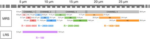
Spectral resolution and wavelength coverages for the LRS and each of the MIRI MRS channels and sub-channels. The full channel ranges of the MRS are listed in the overlapping grey panels towards the top, with the wavelength ranges of each sub-channel are listed below. The purple bar at the bottom shows the wavelength coverage of the LRS. The listed ‘R’ values denote the spectral resolving power (λ/Δλ) for each MRS channel, and the LRS. Image courtesy of N. Lützgendorf (ESA).
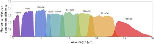
Wavelength coverage of the MIRI imager filters and their photon-to-electron conversion efficiency (PCE) The name of each filter is listed above its range. Their central wavelengths and bandwidths are presented in Table 1. Image courtesy of N. Lützgendorf (ESA).
Filter names, central wavelengths, and bandwidths of the MIRI imager filters.
| Filter name | λ | λ/Δλ |
|---|---|---|
| F560W | 5.6 | 5.0 |
| F770W | 7.7 | 3.5 |
| F1000W | 10.0 | 5.0 |
| F1130W | 11.3 | 16.0 |
| F1280W | 12.8 | 5.0 |
| F1500W | 15.0 | 5.0 |
| F1800W | 18.0 | 6.0 |
| F2100W | 21.0 | 4.0 |
| F2550W | 25.5 | 6.0 |
| Filter name | λ | λ/Δλ |
|---|---|---|
| F560W | 5.6 | 5.0 |
| F770W | 7.7 | 3.5 |
| F1000W | 10.0 | 5.0 |
| F1130W | 11.3 | 16.0 |
| F1280W | 12.8 | 5.0 |
| F1500W | 15.0 | 5.0 |
| F1800W | 18.0 | 6.0 |
| F2100W | 21.0 | 4.0 |
| F2550W | 25.5 | 6.0 |
MIRI consists of an optical bench (containing the optics assembly that includes the imager and MRS) and a cooler unit that keeps the system below 7 K. The MIRI field is selected from the JWST’s focal plane by a single pick off mirror, with the regions of the field directed to each optical function as shown in Fig. 3, adapted from Wright et al. (2015). The spectral resolution and wavelength coverage of both the MRS and LRS are given in Fig. 1. For the LRS, the spectral resolution varies from R ∼ 40 to R ∼ 160 at longer wavelengths (∼10 μm). The MRS wavelength range is covered by four channels, each divided into three sub-bands with the wavelength coverage and spectral resolution shown in Fig. 1. The coronagraphic and LRS prism filters are located in the filter wheel and chosen using the same mechanisms as that for the imager filters. The wavelengths of the imaging filters are shown in Fig. 2, with additional bandwidth information given in Table 1. The flexibility of the system that combines all of the above allows MIRI to make significant contributions to a large range of science topics.
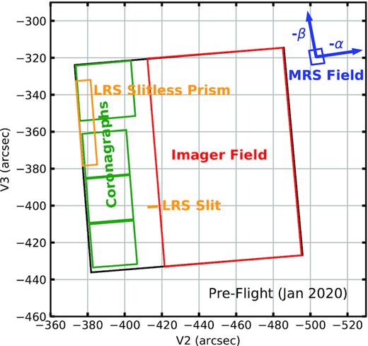
Relative positions of the MIRI components in the JWST focal plane (the v2,v3 coordinate system). The α and β axes of the MRS field (in blue) represent the along and across slice directions of the MRS image slicer (see Wright et al. 2015).
mirisim is a python package developed by the MIRI team to simulate the expected performance of all of MIRI’s modes except coronagraphy. As such, it is able to create realistic simulations of the kinds of science targets described above.
Not only can this simulator be used by the commissioning team to verify new calibrations as the on-orbit performance of the instrument is verified, but it can be used by observers wishing to understand whether their proposed observations will allow them to obtain their science goals, or for theorists to show what their predictions would look like if observed with MIRI.
mirisim is not alone in being able to be used by the community to better understand how an instrument or telescope works, or to demonstrate the relationship between what can be observed and theorists predictions. Notable examples of other simulators that allow the user to simulate their own specific observations include the interferometric simulator for observatories such as ALMA and the JVLA built into casa,1 the imsim 2, and phosim 3 packages for the Rubin Observatory, and the mirage 4 package for NIRCam and NIRISS instruments.
In this paper, we describe the architecture of mirisim (Section 3), and how it simulates MIRI observations. We then give a brief description of how to install and use mirisim in Section 4. We present the outputs of mirisim in Section 5, and conclude in Section 6.
2 SCOPE AND LIMITATIONS
mirisim was designed to replicate, on a best effort basis, the instrument team’s best working knowledge of MIRI. It is expected to reproduce the sensitivity of the instrument to within 10–20 per cent of this ‘nominal’ baseline understanding. It allows for dithered observations, which are often required for JWST calibration pipeline processing, but will not handle mosaiced observations. Very little telescope based spatial information is preserved in an mirisim simulation; simulated observations are centred on (RA,DEC) = (0,0), and the simulator does not account for telescope roll angles. It is based on the Calibration Data Products (CDPs) (see below), and as such, instrumental effects that are not properly captured in CDPs are not captured well in the simulator. This includes effects such as the model of spectral fringing through the instrument, since that is still under development by the MIRI team. It is unclear whether this will be incorporated before launch.
Combined, the above means that science data from the telescope will likely look different from the current understanding available in the simulator. The results from mirisim should be taken as indicative of MIRI performance, and users should continue to use the Space Telescope Science Institute (STScI) exposure time calculator (ETC)5 for a detailed understanding of required exposure times and sensitivities of the observatory.
2.1 MIRI Calibration Data Products
Where possible, the MIRI instrument characteristics are parametrized via the use of MIRI CDPs, which are a set of deliverables to STScI. These data products are the best representation of the instrument, and form the basis of the MIRI calibration reference data system (CRDS) files used in the JWST calibration pipeline.6
In addition to delivering them to STScI, the MIRI team uses these data products within mirisim to characterize the instrument. As CDPs are updated, and new versions incorporated into the pipeline, they are also incorporated into mirisim to provide the most accurate representation of the instrument the team can provide. Whenever there is a change in an underlying CDP, a note is made in the mirisim release notes explaining the versions updates.
3 mirisim COMPONENTS
mirisim is a python package consisting of a number of distinct components, some of which simulate the various light paths through the instrument (ImSim, MIRI–MAISIE, and LRSSim), while others orchestrate (OBSSim), create astronomical scenes (SkySim), and process detector effects (SCASim) for the simulation. A modular approach to the design of mirisim was chosen in order to build flexibility to incorporate increasing detail of the instrument characteristics as hardware was tested. The design of the simulator reflects the modular approach to the hardware and the use of common detectors between the imager and spectrometers. It also facilitates re-use of software modules to build simulators for future instruments. The user interface to mirisim is described in Section 4, but here we describe the individual components that make up the simulator.
For reference, the path through the mirisim components for MRS and imager/LRS simulations are given (respectively) in Figs 4 and 5. In these figures, the flow of data through mirisim starts with users inputting a reference astronomical scene to be simulated, and the observation parameters for the simulation that follow the nomenclature used in the JWST Astronomer’s Proposal Tool (APT).7 The orchestration module (OBSSim) then parses the scene and simulation parameters and sends the commands to the relevant modules that create the sampled scene (or skycube) and then create a model of how the detector would be illuminated (creating an illumination model) this output and the simulation parameters are then passed to the Sensor Chip Assembly simulator (SCASim) where the exposures are calculated, and the final detector images are created. Thus, the final product of an mirisim simulation, regardless of light path, is a detector image. For a description of the detector images, see Section 3.6. ObsSim then wraps the detector images into FITS files with the correct header information so that files can be read by the JWST calibration pipeline.
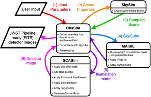
Overview of the path data takes through the MRS version of mirisim. The user supplies input parameters (either at the command line, or from within python), and OBSSim orchestrates the creation of the scene, the dispersion through MAISIE, sending the output illumination model to SCASim, and creating an FITS file of the resultant detector image.
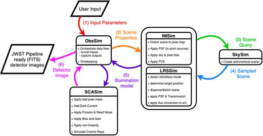
Overview of the path data takes through the imager or LRS versions of mirisim. The user supplies input parameters (either at the command line, or from within python), and OBSSim sends the scene parameters to LRSSim or ImSim to create a scene and determine the illumination model. OBSSim then takes that illumination model (as it does in the MRS case) and passes it to SCASim to create the final detector image, which OBSSim then turns into an FITS file ready for ingest into the JWST calibration pipeline.
Below, we describe the individual mirisim components in greater detail.
3.1 SkySim
The SkySim module creates the astronomical ‘scene’ used by mirisim to simulate the observation with the use of requested instrument setup. A ‘scene’ here is defined as a collection of objects placed within the instrument field of view with spatial and spectral properties that can be mapped into illumination models for the detectors. We use the same terminology here as in the JWST ETC, but allow for more flexibility in the definition of objects within a scene. The user can build up a set of objects to represent what the sky is expected to look like with MIRI.
These ‘scenes’ can take the form of a series of point and extended ‘sources’ (emitters in the field of view) specified by the user with positions, extents, and shapes (for extended objects), and spectral energy distributions (SEDs) of various types. There is also the option to give ascii files containing SEDs for the individual components of the scene. SkySim adds a ‘background’ component to user-defined scenes, which consists of the non-negligible telescope thermal background (see Glasse et al. 2015) as well as other effects such as zodiacal light. It can also read pysynphot SED libraries, which are downloaded as part of the installation process (see Section 4.1) that can be used to populate point or extended objects with library SEDs providing that the SEDs are valid across the required MIRI wavelength range.
SkySim can also interpret user-provided FITS cubes as ready-made input scenes, only requiring a minimal set of FITS header keywords to parse them. Most standard FITS keywords are accepted, with the exception that the wavelength axis must be specified in microns, not Angstroms. Warnings are given if the positional coordinates are not specified properly.
3.2 OBSSim
OBSSim is the mirisim module that orchestrates the rest of the components. It reads in the inputs (via a configuration parser), and ultimately creates the FITS file outputs of each stage of the simulation. It sets up dither positions, coordinates the number of exposures, and keeps track of the timing of the simulated observation to ensure that the header metadata is realistically tracking the time it takes for an observation.
For the MRS light path, OBSSim has the added task of creating a skycube by griding the components of the scene created in SkySim on to a cube object that can then be read by MIRI–MAISIE.
OBSSim is also responsible for processing the illumination model outputs of the three light path simulator components (ImSim, LRSSim, or MIRI–MAISIE) and passing them to the sensor chip assembly simulator (SCASim) along with the observing parameters (number of groups, integration and exposures, whether to simulate SLOW or FAST mode, etc.) input by the user to create the detector image that is the end product of mirisim. Each of these components is described in more detail below (see Sections 3.3–3.6).
3.3 MIRI–MAISIE
MIRI–MAISIE is built using the Multipurpose Astronomical Instrument Simulator Environment (MAISIE; O’Brien et al. 2016) that has been tailored to the MIRI–MRS light path. Its components are based on those of SpecSim (Lorente et al. 2006), and incorporates the transmission, distortion, dispersion, and both the results of the point and line spread function CDPs for MRS observations computed in OBSSim. The output of MIRI–MAISIE is an illumination model (from which OBSSim makes an output FITS file) for each exposure covering the specified (i.e. A, B, and C as shown in Fig. 1) sub-channel of either the ‘Short’ (Ch1–2, 4.8–11.9 μm) or ‘Long’ (Ch3–4, 11.5–28.8 μm) wavelength arms of the MRS, or of both the ‘Short’ and ‘Long’ arms simultaneously. The illumination models are then used by SCASim to create detector images. The bottom right panel of Fig. 7 shows such a detector image for Channels 1a and 2a.
3.4 ImSim
ImSim simulates the light path through the primary imager field of view (i.e. not the LRS or coronagraphs). It queries SkySim to create the astronomical scene to be simulated, determines the FOV to be imaged (i.e. whether to image the full frame or a sub-array), applies the requested filter, distortion sky-flat and photon conversion efficiency (PCE) CDPs, and convolves the scene components with the point spread function (PSF). The resultant illumination model is an intermediate product of mirisim (written out to an FITS file by OBSSim), which is fed (via OBSSim) to SCASim to create a detector image. As seen in Fig. 6, mirisim illumination models and subsequent detector images do show light passing through the coronagraphic fields of view, despite not doing any coronographic simulation.
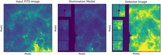
Imager outputs from a 100 frame simulation using filter F1130W (11.3 μm filter), and a WISE image of Carina interpolated to the right wavelength, and moved to a distance of 50 kpc.
During instrument ground testing, a cruciform pattern was seen in the PSF from internal scatterings in the detector. This pattern has been incorporated into the PSF CDPs, and so is not accounted for separately in mirisim. The cruciform is only applied when the target is in field because it is a detector effect.
3.5 LRSSim
The LRS has two modes: slitted and slit-less. LRSSim simulates both of these modes, dispersing the light from the required part of the simulated ‘scene’. Slitless mode is to be used for point sources, and when used in this mode, only the SLITLESSPRISM sub-array (located towards the top left of the detector). In slit mode, the full imager field of view is simulated. The positions of the targets on the detector are shown in fig. 2 of Kendrew et al. (2015). Similarly to ImSim, LRSSim applies transmission, distortion, PCE (or optional spectral response) and PSF CDP (or, optionally the webbPSF model) to the dispersed data to produce an illumination model, which OBSSim then delivers to SCASim to create the final detector images. To support commissioning but also normal observations, LRSSim can optionally simulate the complete detector array to identify possibly disturbing (extended) nearby sources outside the slit or slitless area.
3.6 SCASim
The electronic (pixel gain, dark current, and pixel response) and detector (reset anomaly, last frame effect, droop, and drift) effects of the Sensor Chip Assembly (SCA) itself are described in detail in Ressler et al. (2015). The SCAs for the imager/LRS and MRS detectors are identical (as described in greater detail in Ressler et al. 2015), and as such, the outputs from MAISIE, LRSSim, and ImSim can all be processed by the same simulator module.
The Sensor Chip Assembly simulator (SCASim; Beard et al. 2012) is the final component of mirisim. It simulates the most important MIRI detector effects of the instrument. These include known cosmetic effects (e.g. bad pixels), detector dark current, electronic non-linearity effects, the pixel flat-field, noise sources (e.g. read noise, shot noise) and a plug-in cosmic ray event library (based on Robberto, private communication) which can be updated as our knowledge of these effects improves. The current treatment of cosmic rays is based on the interpixel capacitance corrections of the MIRI detectors as defined by Gaspar (private communication), with refinements subsequently suggested by Rieke (private communication).
SCASim samples the illumination model based on the number of groups, integrations, and exposures requested, applying the noise sources as appropriate. It then returns 3D detector images with slices corresponding to the individual groups for each integration (and sets of images when there are multiple exposures). The detector images represent the sensitivity of the instrument to light, and reproduce, to the teams best understanding, the defects, non-linearities, and noise within the array. These files, when converted to FITS format by OBSSim, and given the appropriate header information, can be read into the JWST calibration pipeline as Level 1B data sets.
4 GETTING AND USING mirisim
4.1 Installation
mirisim has been developed and tested on Apple (macOS) and Linux systems, and the minimum system requirements for running mirisim are comparable to those for the JWST calibration pipeline. The code itself is python 3 based, and mirisim has been bundled into an Anaconda8 environment to ease installation.
Detailed installation instructions for mirisim can be found on the MIRICLE website.9 From this website, users can download an installation script. This self-updating bash script will always download the most recent version of mirisim and install it in a new anaconda environment. The primary environment variables to be set are the location of the CDPs, the PySynPhot libraries, and where mirisim is being installed.
4.2 Usage
There are two ways of interacting with mirisim: at the command line, and from within python itself. Either option can accept (and for command line, requires) user formatted input data files to specify how the simulation should be setup, along with a description of the astronomical scene to simulate. These options are described in more detail below.
4.3 User input files
Whether working at the command line, or from within python, mirisim takes a number of input files which define parameters that define how the astronomical scene is to be setup, what kind of simulation to run, and a number of advanced features (primarily for use in JWST commissioning). These files, and their formatting are described in more detail in the mirisim Users Guide.10 The input files can be used at both the command line, or as inputs into python runs of the simulator. Through the rest of this text, we refer to the scene, simulation, and simulator files with these template names. The scene file (e.g. scene.ini) houses the specification of the astronomical scene to be simulated (e.g. a point source 0.5″ from the field centre with a blackbody SED), and simulation.ini houses the properties of the simulation itself (e.g. which imager filter to use, how many exposures to do, how many groups should be in each integration, etc.).
When running mirisim at the command line, at least one input file is required (simulation.ini), with the understanding that the scene.ini file is specified within the simulation.ini, that it exists, and can be used. Alternatively, a scene file can be specified at run time by simply adding the name of the scene file to the end of the above command. This would override any file named in the simulation input file.
Within python, a scene and a simulation can be built up in a much more dynamic way, by importing the various mirisim components, as described in more detail in the User Guide.
4.4 Formatted input files
The formatting associated with the input files for mirisim takes the same form as those to be used for the JWST Calibration pipeline. An example of the formatting is shown below for setting up the MRS portion of the simulation file:
[Integration_and_patterns]
[[MRS_configuration]]
disperser = SHORT
detector = SW
Mode = FAST
Exposures = 2
Integrations = 2
Frames = 100
The input files consist of sets of named nested groups, with individual properties (e.g. number of integrations to simulate) set within the nested structure provided by the number of square brackets in the section headings.
5 RESULTS
The results of an mirisim simulation are output as FITS files in the same uncalibrated data format that will be delivered to MIRI users, i.e. mirisim results are in the same format as real JWST data, and are readable by the JWST calibration pipeline as 3D ramp data (JWST uncalibrated data format). In accordance with this, the science images are stored in the SCI header extension by default.
mirisim creates an output directory in the current working directory with a pathname that contains the date and time the simulation was started (e.g. yyyymmdd_hhmmss_mirisim). In that directory, copies are made of the scene.ini and simulation.ini files used to drive the simulation (or created if the simulation was manually built within python), and a number of subdirectories are created depending on the type of simulation performed. For all optical paths, directories are created for intermediate product illumination models (illum_models) and final product detector images (det_images). The illumination models are the outputs of ImSim, LRSSim, or MIRI–MAISIE, which show how the detector is to be illuminated. The detector images are the final outputs of mirisim: the illumination models that have been processed through SCASim, and saved to JWST calibration pipeline ready FITS files. Examples of the illumination models and detector images for the imager, MRS, and LRS are given in Figs 6, 7, and 8 (respectively).
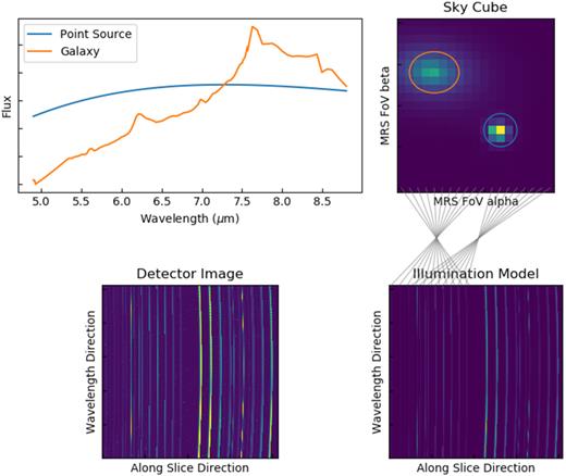
MRS outputs from a 100 frame simulation showing Top Left: Spectra of the two targets (a point source and an extended ellipse with blackbody and galaxy spectra, respectively). Top Right: Locations of the two targets in the MRS field of view. Bottom Right: Model of how the detector is being illuminated by the scene. The grey lines between the top and bottom right-hand panels indicate how the slices in Channel 1A are mapped to the left portion of the detector. Bottom Left: Final detector image (in JWST Level 1B data format) of the simulation.
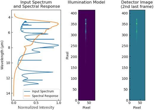
LRS slitless outputs for a 100 frame simulation showing a point source with a spectrum of a PDR.
For MRS simulations, a third directory is created for datacubes (skycubes). These cubes are used by MIRI–MAISIE to disperse light into the illumination models. The skycubes can also help the user understand what their astronomical scene looked like before the light was dispersed.
5.1 Example mirisim simulations
5.1.1 Imager example
Fig. 6 shows an example of an imager simulation. The input for the simulation was an interpolation of data from bands 2 and 3 of the WISE data of the Carina nebula (Wright et al. 2010). A linear interpolation of the 4.6 and 12.2 μm data was created to simulate 11.3 μm observations, and the spatial resolution information in the header was modified to represent higher resolution data (i.e the cdelt parameters were changed from ∼1.37″ to ∼0.06″). The resultant FITS file is shown in the left-hand panel of Fig. 6. The middle panel shows the model of the illumination presented to the detector through the imager field of view. The right-hand panel shows the resultant final data product of an imager simulation. The simulation parameters used here consisted of using F1130W with the full imager field of view to observe 100 groups in a single integration using FAST mode. The detector image shown here is the second last group/frame captured in the simulated 3D ramp data at a single dither position.
5.1.2 MRS example
Fig. 7 shows an example of an MRS simulation. Here, the input is built up of individual components created within SkySim. The first is an extended object (elliptical galaxy) with an effective radius of 1″, a Sersic index of 1, and an axial ratio of 0.5 placed at a position angle of 85 deg. The SED of NGC 1068 was then applied to the extended object. The SED was populated using the Brown atlas within pySynPhot (Brown et al. 2014). The galaxy and its SED are highlighted in orange in the top two panels of Fig. 7 that show the spectral (left) and spatial (right) distributions of the objects. The other target placed in the MRS field of view was a point source with a blackbody SED and characteristic temperature of 700 K. This target, and its SED are highlighted in blue in the top two panels of Fig. 7. As with the imager above, the example MRS simulation consisted of 100 integrations in a single exposure, however, here we used SLOW mode readouts. Only the ‘SHORT’ wavelength arm (Channels 1 and 2) was simulated, and all results here are for the ‘A’ sub-channel. This means that the images in the bottom panels of Fig. 7 show the data from 1A and 2A only, with 1A shown in the left half of each figure, and 2A shown in the right. The grey lines between the skycube (top right) and illumination model (bottom right) panels show how the image slices are mapped to the detector in Channel 1. Similar lines could be drawn for ch2a (to map to the right portion of the illumination model), but were left out for clarity.
5.1.3 LRS slitless mode example
Fig. 8 shows the outputs of an LRS slitless simulation in which a point source was placed at the ‘source’ position for the slitless spectrograph (see fig. 2 of Kendrew et al. 2015). It was given the PDR spectrum shown in blue in the left-hand panel of Fig. 8, and the resultant illumination model is shown in the middle panel. The LRS spectral response is also shown (in orange) in the left-hand panel of the figure to show why the longer wavelength spectral features of the PDR spectrum are not as prominent in the spectral trace provided in the middle panel. The right-hand panel of Fig. 8 shows the 2nd last group/frame of the 3D detector image resulting from a single integration of 100 groups using the FAST readout mode. The imager filter wheel was set to the P750L filter, and the sub-array to readout was set to SLITLESSPRISM.
6 CONCLUSIONS
mirisim is the simulator developed by the MIRI instrument team that reproduces the expected on-orbit performance of the instrument. It simulates each of the light paths through MIRI with the exception of coronagraphy. It is built in python, and comes bundled in an Anaconda environment that incorporates all of its dependencies. It can be used both at the command line, or interactively in a python shell. It draws on the CDPs developed by the MIRI team as we characterize the instrument.
The products of mirisim are FITS files with valid metadata and header information that allow them to be ingested into the JWST pipeline as if they were true MIRI data.
mirisim is expected to be used for various purposes by a broad range of communities. For instance, it will be used by the instrument team during commissioning to correlate observations with expected performances and help refining our understanding of the instrument. It can be used by prospective JWST users to understand the noise characteristics they should expect when imaging faint targets, while others may find it useful to familiarize themselves with data formats from the instrument, to aid in developing observing plans, or for producing realistic inputs when training in data processing and analysis using the JWST calibration pipeline. It can also be used by modellers who want to show how their model predictions could be tested with MIRI observations.
ACKNOWLEDGEMENTS
The authors would like to thank the anonymous referee for their suggestions that have improved the clarity of this manuscript. The acknowledgements were compiled using the Astronomy Acknowledgement Generator. This research made use of Astropy, a community-developed core python package for Astronomy (Astropy Collaboration 2013, 2018) This publication makes use of data products from the Wide-field Infrared Survey Explorer (Wright et al. 2010), which is a joint project of the University of California, Los Angeles, and the Jet Propulsion Laboratory/California Institute of Technology, funded by the National Aeronautics and Space Administration.
DATA AVAILABILITY
No new data were generated or analysed in support of this research. Instructions for downloading the mirisim code can be found in Section 4.
