


ABSTRACT
The 21-cm absorption feature reported by the EDGES collaboration is several times stronger than that predicted by traditional astrophysical models. If genuine, a deeper absorption may lead to stronger fluctuations on the 21-cm signal on degree scales (up to 1 K in rms), allowing these fluctuations to be detectable in nearly 50 times shorter integration times compared to previous predictions. We commenced the ‘AARTFAAC Cosmic Explorer’ (ACE) program, which employs the AARTFAAC wide-field image, to measure or set limits on the power spectrum of the 21-cm fluctuations in the redshift range z = 17.9–18.6 (Δν = 72.36–75.09 MHz) corresponding to the deep part of the EDGES absorption feature. Here, we present first results from two LST bins: 23.5–23.75 and 23.75–24.00 h, each with 2 h of data, recorded in ‘semi drift-scan’ mode. We demonstrate the application of the new ACE data-processing pipeline (adapted from the LOFAR-EoR pipeline) on the AARTFAAC data. We observe that noise estimates from the channel and time-differenced Stokes V visibilities agree with each other. After 2 h of integration and subtraction of bright foregrounds, we obtain 2σ upper limits on the 21-cm power spectrum of |$\Delta _{21}^2 \lt (8139~\textrm {mK})^2$| and |$\Delta _{21}^2 \lt (8549~\textrm {mK})^2$| at |$k = 0.144~h\, \textrm {cMpc}^{-1}$| for the two LST bins. Incoherently averaging the noise bias-corrected power spectra for the two LST bins yields an upper limit of |$\Delta _{21}^2 \lt (7388~\textrm {mK})^2$| at |$k = 0.144~h\, \textrm {cMpc}^{-1}$|. These are the deepest upper limits thus far at these redshifts.
1 INTRODUCTION
Observations of the redshifted 21-cm signal of neutral hydrogen from the Cosmic Dawn (CD) and Epoch of Reionization (EoR) hold the potential to revolutionize our understanding of how these first stars and galaxies formed and the nature of their ionizing radiation (Madau, Meiksin & Rees 1997; Shaver et al. 1999; Furlanetto, Oh & Briggs 2006; Mesinger, Furlanetto & Cen 2011; Pritchard & Loeb 2012; Zaroubi 2013). During the CD (12 ≲ z ≲ 30), the first luminous objects formed in the dark and neutral Universe (Pritchard & Furlanetto 2007). X-ray and ultraviolet radiation from these first stars heated and ionized neutral hydrogen (H i) in the surrounding inter-galactic medium (IGM) during the EoR. This process continued (spanning the redshift range 6 ≲ z ≲ 12) until hydrogen in the IGM became fully ionized (Madau et al. 1997).
In recent years, a large number of observational efforts got underway to observe this faint 21-cm signal from the CD and EoR. Radio interferometers such as the Giant Meterwave Radio Telescope (GMRT; Paciga et al. 2011), the LOw Frequency ARray (LOFAR; van Haarlem et al. 2013), the Murchison Widefield Array (MWA; Bowman et al. 2013; Tingay et al. 2013), the Precision Array for Probing the Epoch of Reionization (PAPER; Parsons et al. 2010) as well as the next-generation instruments such as the Hydrogen Epoch of Reionization Array (HERA; DeBoer et al. 2017), the Long Wavelength Array (LWA; Greenhill et al. 2012), the New Extension in Nançay Upgrading loFAR (NENUFAR; Zarka et al. 2012), and the upcoming Square Kilometre Array (SKA; Mellema et al. 2013; Koopmans et al. 2015) are working towards measuring the spatial brightness temperature fluctuations in the high-redshift cosmological 21-cm signal.
In parallel, single-element radiometers such as the Experiment to Detect the Global Epoch of Reionization Signature (EDGES; Bowman et al. 2018), the Large-aperture Experiment to Detect the Dark Ages (LEDA; Bernardi et al. 2016), the Shaped Antenna measurement of the background RAdio Spectrum 2 (SARAS 2; Singh et al. 2017), the Sonda Cosmológica de las Islas para la Detección de Hidrógeno Neutro (SCI-HI; Voytek et al. 2014), the Probing Radio Intensity at high z from Marion (PRIZM; Philip et al. 2019), and the Netherlands-China Low frequency Explorer1 (NCLE) are seeking to measure the global sky-averaged 21-cm signal as a function of redshift.
In 2018, a deep spectral feature centred at 78 MHz was reported by the EDGES collaboration (Bowman et al. 2018). The feature was presented as the long sought-after 21-cm absorption feature seen against the CMB during the CD at z ∼ 17. The location of this putative absorption trough is consistent with redshift predictions from theoretical models and simulations of the CD (Furlanetto et al. 2006; Pritchard & Loeb 2010; Mesinger, Ferrara & Spiegel 2013; Cohen et al. 2017). However, the depth of the feature is ΔT21 ∼ 0.5 K (|$99{{\ \rm per\ cent}}$| confidence level), which is two to three times stronger and considerably wider (Δν ∼ 19 MHz) than that predicted by the most optimistic astrophysical models (e.g. Pritchard & Loeb 2010; Fialkov, Barkana & Visbal 2014; Fialkov & Loeb 2016; Cohen et al. 2017). Moreover, the observed feature is flat-bottomed instead of a smooth Gaussian-like shape. Several ‘exotic’ theoretical models have already been proposed which might explain the depth of the feature, such as a considerably colder IGM due to interaction between baryons and dark matter particles causing a lower spin-temperature and therefore a deeper absorption feature (e.g. Barkana 2018; Fialkov, Barkana & Cohen 2018), or a stronger radiation background against which the absorption is taking place (e.g. Dowell & Taylor 2018; Ewall-Wice et al. 2018; Feng & Holder 2018; Fialkov & Barkana 2019). Although the 21-cm signal is expected to be stronger at these redshifts, the foreground emission is several times brighter at these frequencies compared to EoR 21-cm signal observations at 150 MHz (Bernardi et al. 2009, 2010). Moreover, ionospheric effects are amplified at lower frequencies (de Gasperin et al. 2018; Gehlot et al. 2018), rendering the measurement of the signal equally (or even more) challenging than in EoR experiments. As of now, Ewall-Wice et al. (2016) reported a systematics-limited power spectrum upper limit of |$\Delta _{21}^2 \lt (10^4~\text{mK})^2$| on co-moving scales |$k\lesssim 0.5~h\, \text{cMpc}^{-1}$| (in 3 h of integration) on the 21-cm signal brightness temperature in the redshift range 12 ≲ z ≲ 18 using MWA. This overlaps with the low-redshift edge of the 21-cm absorption feature (Bowman et al. 2018). Gehlot et al. (2019) provided a 2σ upper limit of |$\Delta _{21}^2 \lt (1.4\times 10^4~\text{mK})^2$| on the 21-cm signal power spectrum at |$k = 0.038~h\, \text{cMpc}^{-1}$| (in 14 h of integration) using the LOFAR-Low Band Antenna (LBA) system in the redshift range 19.8 ≲ z ≲ 25.2, which corresponds to the high-redshift edge of the absorption feature. More recently, Eastwood et al. (2019) used OVRO-LWA observations to report a 2σ upper limit of |$\Delta _{21}^2 \lt (10^4~\text{mK})^2$| at |$k \approx 0.1~h\, \text{cMpc}^{-1}$| (in 28 h of integration) at redshift z ≈ 18.4.
Although concerns have been raised about the validity of the detection of the absorption feature in terms of foreground modelling and instrumental effects (Hills et al. 2018; Bradley et al. 2019), if the detection is confirmed, the strength of the 21-cm absorption feature can also cause a significant increase in the 21-cm brightness temperature fluctuations in the redshift range z = 17–19 (Barkana 2018; Fialkov et al. 2018). This redshift range corresponds to the deepest part of the absorption profile. It enables detection of the 21-cm signal brightness temperature fluctuations on degree angular scales in this redshift range within a much shorter integration time (∼50 times shorter) compared to what was previously expected.
Motivated by this, we have commenced a large-scale program called ‘AARTFAAC Cosmic Explorer’ (ACE) to measure or limit the power spectrum of the brightness temperature fluctuations of the 21-cm signal from z ∼ 18 using the LOFAR Amsterdam-ASTRON Radio Transients Facility And Analysis Centre (AARTFAAC) wide-field imager (Prasad et al. 2016). AARTFAAC correlates up to 576 individual receiver elements [LBA dipoles or High Band Antenna (HBA) tiles] in the core of LOFAR, thereby providing a wider field of view (FoV) and increased sensitivity on large angular scales compared to regular LOFAR observations. The redshift range targeted by ACE is z = 17.9–18.6 (72.36–75.09 MHz frequency range), which corresponds to the deep part of the EDGES absorption feature. The ACE programme2 has collected about 500-h deep integration data of a large part of the northern sky to measure the power spectrum. In this work, we present first power spectrum results in two LST bins each with 2 h of data and successfully demonstrate the end-to-end application of the new ACE data-processing pipeline, which is adapted from the LOFAR-EoR data processing pipeline to AARTFAAC data. Readers may refer to Patil et al. (2017), Gehlot et al. (2019), and Mertens et al. (2020) for an overview of the LOFAR-EoR data processing pipeline, and a description of HBA and LBA data processing.
This paper is organized as follows: Section 2 briefly describes the AARTFAAC wide-field imager, the observation setup of ACE observations, and the basic pre-processing steps for the raw data, e.g. flagging and averaging. The calibration and imaging strategy for the ACE data is described in Section 3. In Section 4, we estimate and discuss the noise in ACE data and method of combining multiple ACE observations. In Section 5, we describe the Gaussian Process Regression foreground removal technique and power spectrum estimation methodology. We discuss results from the analysis Section 6. Finally, we summarize the work and discuss future outlook in Section 7. We use Lambda cold dark matter cosmology throughout the analyses with cosmological parameters consistent with Planck (Planck Collaboration XIII 2016).
2 OBSERVATIONS AND PRE-PROCESSING
We used the LOFAR-AARTFAAC wide-field imager to observe the northern sky in the frequency range 72.4–75 MHz. The sky was observed in ’semi drift-scan’ mode,3 and the observed snapshot data was processed using a tweaked version of the LOFAR-EoR data processing pipeline (Gehlot et al. 2018, 2019; Mertens et al. 2020). The observational setup and the pre-processing steps are briefly described in following subsections.
2.1 The LOFAR AARTFAAC wide-field imager
The AARTFAAC is a LOFAR-based all-sky radio transient monitor (Prasad et al. 2016; Kuiack et al. 2019). It piggybacks on ongoing LOFAR observations and taps the digital signal streams of individual antenna elements from 6 to 12 core stations depending on the requirements. AARTFAAC operates in two modes viz. A6 where the six innermost stations (also called the ‘superterp’) of the LOFAR-core are used, and A12 that employs 12 innermost stations of the LOFAR-core. The A6 mode consists of 288 dual-polarization receivers (e.g. LBA dipoles or HBA tiles) within a 300-m diameter circle, and the A12 mode consists of 576 such receivers spread across 1.2 km (van Haarlem et al. 2013). Fig. 1 shows the 15-min synthesis uv-coverage of the A12 mode at 74 MHz and the radial profile (Nvis per baseline bin of |$d\boldsymbol{u} = 0.5\lambda$|) of the uv-coverage. The latter is relatively flat for |$\boldsymbol{u} = 10\!-\!100\lambda$| except for a dip around |$\boldsymbol{u}\sim 20\lambda ,\, 70\lambda$|, which is due to slightly patchy LBA-dipole layout in the ‘superterp’ and the transition to non-superterp baselines. The array is co-planar at centimetre level within 0–70λ, which is beneficial for wide-field imaging. In addition to this, the baselines up to 1.2 km support intermediate-resolution imaging, which helps to improve calibration and better captures compact structure in the sky. Each of the inner 12 LOFAR core stations consists of 96 LBA dipoles4 (only 48 out of 96 dipoles can be used at a time) and 48 HBA tiles.5 At a given time, AARTFAAC can only observe in either LBA or HBA mode depending upon the ongoing LOFAR observation. The digitized signal from the corresponding receiver elements is tapped and transported to the AARTFAAC correlator (located at the Centre for Information Technology (CIT)6 in Groningen, Netherlands) prior to beam-forming. Due to network limitations, only 16 subbands can be correlated using the 16-bit mode. Each subband is 195.3 kHz wide and consists of up to 64 channels providing a maximum frequency resolution of 3 kHz, with currently maximum instantaneous system bandwidth of 3.1 MHz. The correlator subsystem is a GPU based and produces correlations (XX, XY, YX, YY) for all dipoles pairs for every frequency channel with 1-s integration. The correlator has 1152 input streams with 576 signal streams per polarization. The output correlations can either be dumped as raw correlations on storage discs on the AARTFAAC storage/compute cluster or can be routed to the AARTFAAC real-time calibration and imaging pipeline for transient detection. AARTFAAC can only observe in drift-scan mode. However, phase tracking can be applied to raw data during or after pre-processing. The raw data from the AARTFAAC storage/compute cluster can be streamed via a fast network (1 Gbit s−1) to the LOFAR-EoR processing cluster ‘Dawn’ at the CIT. The raw data can be converted to standard measurement set (MS) format using a custom software package aartfaac2ms 7 (Offringa et al. 2015), which can also apply offline phase tracking. Readers may refer to Prasad et al. (2016) for further information about AARTFAAC system design and capabilities, and van Haarlem et al. (2013) for observing capabilities of LOFAR.
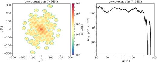
The left-hand panel shows the uv-coverage of A12 mode (12 station configuration) of the LOFAR-AARTFAAC LBA array at 74 MHz for 15 min of synthesis. The right-hand panel shows the radial profile of the uv-coverage, i.e. Nvis per baseline bin (|$|\boldsymbol{u}| =\sqrt{u^2+v^2}$|) of width 0.5λ.
2.2 ACE observational setup and status
We use the A12 mode of AARTFAAC to observe the Northern sky in the drift-scan mode with the mean phase centre at the zenith. We use 14 contiguous subbands (a total of 2.73-MHz bandwidth) to observe the 72.36–75.09 MHz, targeting the redshift range z = 17.9–18.6. We place the two remaining subbands ∼4 MHz away from the targeted band centre on either side of the band, to aid in assessing the wide-band systematics and calibration quality as well as help foreground modelling and subtraction. We choose three channels per subband (with 65.1-kHz resolution) and 1-s correlator integration. High spectral and time resolution provides improved RFI excision and a better handle on delay/frequency transform (discussed in Section 5.3). The ACE observing campaign concluded after observing around 500 h of northern sky in drift-scan mode during three LOFAR observing cycles. Most observations span night time LSTs with a typical span of 4–12 h per observation.
For this pilot analysis, we select two LST bins, viz 23.5–23.75 (LST:23.5 h or LST-bin 1 hereafter) and 23.75–24.00 h (LST:23.75 h or LST-bin 2 hereafter) with eight observation blocks of 15 min each, taken from different nights recorded during first cycle observations. This corresponds to the total integration time of 2 h per LST-bin. Table 1 summarizes the observational and correlator setting details.
Observational and correlator setting details.
| Parameter | Value |
|---|---|
| Telescope | LOFAR AARTFAAC |
| Observation cycle and ID | Cycle 10, LT10_006 |
| Antenna configuration | A12 |
| Number of receivers | 576 (LBA dipoles) |
| Sidereal bins (h) | 23.5–23.75 and 23.75–24.00 h |
| Number of observation blocks (per LST-bin) | 8 |
| Phase centre | Bin 1: RA 23h37m30s, Dec. +52d38m00s |
| Bin 2: RA 23h52m30s, Dec. +52d38m00s | |
| Minimum frequency | 72.36 MHz |
| Maximum frequency | 75.09 MHz |
| Target bandwidth | 2.73 MHz |
| Outrigger subbands | 68.36 and 78.90 MHz |
| Primary beam FWHM | 120○ at 74 MHz |
| Field of view | 11 000 deg2 at 74 MHz |
| Polarization | Linear X–Y |
| Time, frequency resolution: | |
| Raw data | 1 s, 65.1 kHz |
| After flagging and averaging | 4 s, 65.1 kHz |
2.3 Data pre-processing
The first step of data processing is to apply tracking to the drift-scan observations. For instruments with much wider FoVs (full width at half-maximum ∼ 120○ in our case), phase referencing to a single stationary point in the sky during long observations limits the portion of the sky which is visible. This is not an optimal strategy for long-duration observations. Therefore, instead of fixing the phase reference to a single stationary point for the entire observation, we choose to re-phase every 15-min observation block. The phase centre for each observation block is a constant declination point (on a great circle through zenith) that passes through zenith mid-way during the 15-min observation. We refer these re-phased 15-min observation blocks as ‘time-slices’ throughout this paper.
The next step is RFI excision, which is performed on the highest resolution data to minimize information loss. We use aoflagger (Offringa et al. 2010; Offringa, van de Gronde & Roerdink 2012) to perform RFI excision on raw data and also flag all visibilities that include non-working LBA dipoles (|$\sim \! 6\!-\!7{{\ \rm per\ cent}}$|). The remaining data are averaged to a resolution of 4 s and 65.1 kHz and subsequently divided into 15-min time-slices for every individual phase centre. Each time-slice is separately written into MS format, which are stored permanently on the LOFAR-EoR processing cluster. The data volume in MS format is around 150 GB for 15-min time-slices, and ∼1.2 TB for 2 h worth of data, respectively. The aartfaac2ms package performs the re-phasing and flagging tasks and returns the phased and flagged data in MS format. The dipoles within a station share the same electronic cabinets, such that intra-station baselines may be affected by mutual-coupling/cross-talk effects. Therefore all intra-station baselines (|$|\boldsymbol{b}| \lesssim 80\, \text{m}$|) are also flagged post-MS conversion. The fraction of visibilities flagged by aoflagger (excluding non-working dipoles), at this stage, varies between 2 and 25 per cent for different time-slices in the two LST bins.
3 CALIBRATION AND IMAGING
Visibilities measured by AARTFAAC are corrupted by the errors caused due to instrumental imperfections such as complex receiver gain, primary-beam and global band-pass, as well as environmental effects, for example, due to the ionosphere. Calibration of AARTFAAC refers to the estimation of these errors and correcting the observed visibilities to obtain a reliable estimate of the true sky visibilities. The errors that corrupt the visibilities can be classified into two broad categories: direction-independent (DI) errors and direction-dependent (DD) errors. DI errors are independent of the direction of the incoming signal from the sky and comprise of complex receiver gain and frequency band-pass, as well as a global ionospheric phase. In contrast, DD errors change with sky direction, e.g. as a result of the antenna beam pattern, ionospheric phase fluctuations, and Faraday rotation (Hamaker, Bregman & Sault 1996; Sault, Hamaker & Bregman 1996; Smirnov 2011a,b).
3.1 DI calibration
DI calibration involves estimation of complex gains (full-Jones) per dipole, per time and frequency interval (represented by a complex 2 × 2 Jones matrix for two linear polarizations). We use dppp 8 to calibrate the raw visibilities and subsequently apply the gain solutions obtained in the calibration to the visibilities. Unlike sagecal-co (Yatawatta 2015; Yatawatta 2016; Yatawatta, Diblen & Spreeuw 2017) that we used previously in Gehlot et al. (2019) for LBA-beam-formed data, dppp employs the primary beam model for individual LBA dipoles. We use Cas A and Cyg A (the two brightest sources in the northern sky) to calibrate the visibilities. Their sky model consists of 14 components (9 components for Cas A and 5 components for Cyg A), i.e. Delta functions and Gaussians. The models of these sources were obtained using LOFAR-LBA observations and the source fluxes in the model, within a few per cent, are consistent with the Very Large Array (VLA) observations at 74 MHz (Cohen et al. 2007; Kassim et al. 2007). We use a power law with a spectral index of −0.8 to represent the source spectra. We choose a calibration solution-time interval of 16 s for each 65.1-kHz channel to account for DI (or beam-averaged) instrumental and slower ionospheric effects while maintaining a reasonable signal-to-noise ratio (∼30) over the calibration interval. During calibration, we exclude the baselines |$|\boldsymbol{u}| \lt 20\lambda$| in order to avoid the large-scale diffuse Galactic emission biasing the calibration solutions. We apply a LOFAR-LBA dipole beam model9 during the model prediction step to adjust the flux scale. Absolute flux scale can be obtained by applying the beam model before the imaging step. Although the current sky model is somewhat limited in terms of the number of sources, it represents most of the flux on the baselines used for later analyses. We are working on developing a more accurate sky model for calibration, which will include compact sources above the confusion limit and multiscale diffuse emission for robust calibration of AARTFAAC.
3.2 DD calibration
The two brightest sources Cas A and Cyg A dominate the visibilities and superpose significant PSF side-lobes over the field. It is crucial to subtract these sources to reduce the confusion due to these side-lobes. We use dppp (DDEcal) to subtract these sources using DD calibration. We use a calibration solution interval of 16 s and 65.1 kHz, respectively. The calibration is constrained in the frequency direction and enforces frequency smoothness at 2-MHz level. This is somewhat similar to consensus optimization in sagecal-co (Yatawatta 2016; Yatawatta et al. 2017), which also enforces frequency smoothness of gain solutions. We exclude baselines |$|\boldsymbol{u}| \lt 60\lambda$| in this step to reduce bias due to source subtraction on smaller baselines used for analyses in later sections. The directional gain solutions obtained towards Cas A and Cyg A are used to subtract them.
After this, we perform another flagging step where we flag dipoles with relatively high visibility variance in time and frequency. We use aoquality and aoqplot (bundled with aoflagger) to generate quality statistics and flag dipoles with five times more variance compared to the average. Subsequently, we run aoflagger and SSINS- (Sky Subtracted Incoherent Noise Spectra; see Wilensky et al. 2019 for more details) based flagger to flag visibilities with bad (non-converged) solutions and corrupted by low-level RFI, respectively. After this intermediate flagging step, we re-perform the DI, and DD calibration steps in Sections 3.1 and 3.2, respectively. Finally, another instance of aoflagger is run to remove any remaining visibilities with bad/non-converged calibration solutions. After two rounds of flagging, the final fraction of flagged visibilities in the 20–50λ baseline range amounts to 4.5–7 per cent for different nights in the LST:23.5-h bin, and 4–6 per cent in the LST:23.75-h bin (except for two nights in the second bin, where flagged visibilities fractions are around 9 and |$14{{\ \rm per\ cent}}$|, respectively).
3.3 Imaging
The visibilities after DI, DD-calibration. and iterative flagging are imaged with wsclean package (Offringa et al. 2014; Offringa & Smirnov 2017), a wide-field interferometric imaging software that uses the w-stacking algorithm. We use a ‘Kaiser-Bessel’ kernel (Kaiser & Schafer 1980), which is an approximation of the Prolate Spheroidal Wave Function (Jackson et al. 1991), for gridding with a kernel-size of 31 pixels with an oversampling factor of 1.6 × 10⁴ and a padding factor of 1.5 to avoid any artefacts due to gridding. Readers may refer to Offringa et al. (2019) for a detailed analysis of convolutional gridding artefacts, their impact on 21-cm power spectra and methods to mitigate these artefacts. We use the 20–60λ baseline range with ‘natural’ weighting scheme to produce Stokes I, V, and PSF images for all channels and time-slices over the full visible sky for further analysis. The image cubes produced by wsclean are converted to gridded visibilities in brightness temperature units of Kelvin. The cubes are trimmed to |$120{^\circ }$| size using a ‘Hann’10 spatial taper (see e.g. Blackman & Tukey 1958) and 25–40λ baseline range for further analyses. These gridded visibility cubes (|$\mathcal {V}(u,v,\nu)$|), number of visibilities per uv-cell (N(u, v, ν)), and other related metadata are stored in HDF5 data format.11 Fig. 2 shows a higher resolution deep-cleaned Stokes I continuum image (using all baselines with ‘Briggs 0.5’ weighting scheme) corresponding to the LST:23.5-h bin. We observe that subtraction of the bright sources Cas A and Cyg A leaves residuals at the |$\sim \! 1\!-\!2{{\ \rm per\ cent}}$| level.
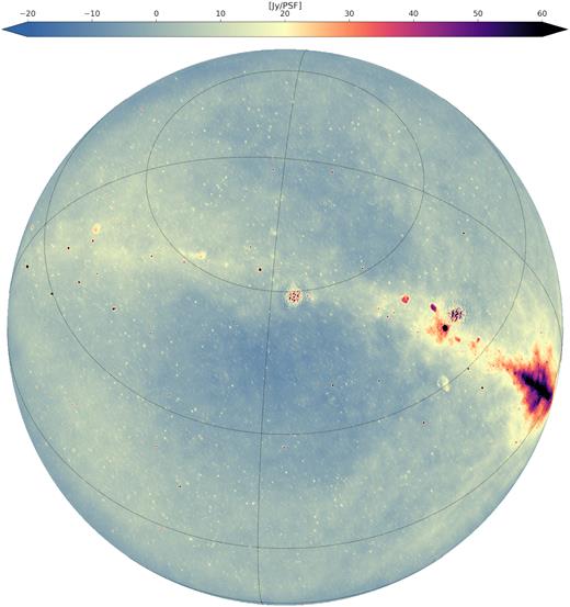
Intermediate resolution Stokes I continuum image (72.4–75.1 MHz, single night, cleaned) of LST:23.5-h bin used in the analysis. The image is shown in orthographic projection, where dotted curves represent the parallels and meridians corresponding to Dec. (30○ separation) and RA, respectively.
We also produced another set of higher resolution Stokes I snapshot images of the calibrated data with 1-min integration per snapshot, for every night used in the analysis, to study the ionospheric condition during these observations. A lower baseline cut is applied to avoid the large-scale Galactic diffuse emission. A source data base was created by selecting ∼2500 compact sources from the combined image of all nights using pybdsf software (Mohan & Rafferty 2015). The sources from the data base were matched in snapshot images using pybdsf and position shifts corresponding to 650 bright sources (out of 2500) were obtained. These position shifts are used in later sections to assess ionospheric conditions for different nights.
4 NOISE STATISTICS
where σvis and Nvis are visibility noise and number of visibilities per uv-cell, respectively. Also, Δν and Δt are the frequency channel width and time resolution, respectively. We found the average SEFD values for LST bins 1 and 2 to be |$\approx \! 1.93\,$| (|$\pm 33\,$|kJy) and |$\approx \! 1.95\,$| MJy (|$\pm 49\,$|kJy), respectively. These estimates are similar (within a few per cent) to other SEFD estimates for AARTFAAC imager (|$\approx \! 2\,$|MJy12). Differencing Stokes V visibilities corresponding to adjoining channels (|$\delta _{\nu } \mathcal {V}_{V}(u,v,\nu)$|) also provides an estimate of frequency uncorrelated noise. We compare the ratio of frequency averaged angular power spectra (|$\langle C_{\ell }[\delta _{\nu } \mathcal {V}_{V}] \rangle / \langle C_{\ell }[\delta _t \mathcal {V}_{V}]\rangle$|) of time and frequency difference Stokes V visibilities. Fig. 3 shows the ratio for eight nights in the two LST bins. We observe that the ratio varies between 1.0 and 1.2 for different nights in either LST bins. However, the mean of ratios for different nights varies between 1 and 1.1 and shows a weak baseline dependence. We suspect that the excess is due to the residual part of the Stokes I sky leakage to Stokes V (at 0.2 per cent level at 74 MHz in Stokes I) in channel difference visibilities which is coherent over different nights. The residual sky is small enough and is of the order of the thermal noise for a single time-slice, however, appears in the incoherent mean of the ratio. The baseline dependence might be caused by the scale dependence of the residual sky emission.
![Ratio of frequency averaged angular power spectra of frequency and time difference visibilities. The left-hand panel shows $\langle C_{\ell }[\delta _{\nu } \mathcal {V}_{V}] \rangle _t / \langle C_{\ell }[\delta _{t} \mathcal {V}_{V}]\rangle _{\nu }$ for different nights in the LST:23.5-h bin. The right-hand panel is same as the left-hand panel but for the LST:23.75-h bin. The black curve shows the mean of the ratios for eight nights.](https://oup.silverchair-cdn.com/oup/backfile/Content_public/Journal/mnras/499/3/10.1093_mnras_staa3093/1/m_staa3093fig3.jpeg?Expires=1750350415&Signature=DC4~cYVDp3ayStotd-87jmGi1cHYlV6gr4snPa6POA30tvuu05NCwz8iEHxE-k3fNSE0r5rKR93iOfsAT~JBzsGc-9I2sDA~6qabAFLALxSn9x~-osVz8gcpdY9Szh5rhvorTsi8aGhYSi81UbW63h~iTQIS8z~oaKQDkyKGXaWd7k004z-aUj4q8b9gWacQncT5OIa4OXIN6mE0nAeidcGWv13m11ZqQxcWlPxIvNGlT4NJ18Ltlwhr~~MFR~THv18j0AI9R6i4Het~~HBCvvzXek-vx1XnWKX~E4C-5Ig30~rQs6RtcEWLSHqFci8TPvwX1ldQsuOQ72lQtGusAA__&Key-Pair-Id=APKAIE5G5CRDK6RD3PGA)
Ratio of frequency averaged angular power spectra of frequency and time difference visibilities. The left-hand panel shows |$\langle C_{\ell }[\delta _{\nu } \mathcal {V}_{V}] \rangle _t / \langle C_{\ell }[\delta _{t} \mathcal {V}_{V}]\rangle _{\nu }$| for different nights in the LST:23.5-h bin. The right-hand panel is same as the left-hand panel but for the LST:23.75-h bin. The black curve shows the mean of the ratios for eight nights.
We use channel difference visibilities as a proxy for frequency uncorrelated noise and time difference visibilities as a proxy of thermal noise in the data. Previous LOFAR-EoR data analyses in Patil et al. (2017) and Gehlot et al. (2019) used Stokes V data itself as a noise estimator because only a tiny fraction of sky is circularly polarized making Stokes V a proxy of thermal noise of the system. However, in wide-field arrays such as AARTFAAC, the Stokes I to Stokes V polarization leakage can become more significant, contaminating the otherwise clean Stokes V data. Another thermal noise estimator is time-differenced Stokes V visibilities as described above; however, it does not account for uncorrelated errors in the frequency direction. Therefore, we simulate noise using equation (1), with SEFD estimates based on channel differenced Stokes V visibilities. Associated noise visibilities |$\mathcal {V}_{\text{N}}(u,v,\nu)$| are later used to correct for the noise bias in Stokes I residual power spectra. This approach is similar to the one used by Mertens et al. (2020) to simulate noise visibilities.
4.1 Combining multiple time-slices
5 FOREGROUND REMOVAL
Subtraction/isolation of the bright foreground emission is a crucial step in 21-cm signal experiments. The intrinsic foreground emission has two dominant components viz. diffuse emission (Galactic synchrotron and thermal emission), and extra-galactic sources (e.g. radio galaxies, clusters and supernova remnants; Di Matteo et al. 2002; Zaldarriaga, Furlanetto & Hernquist 2004; Bernardi et al. 2009; Ghosh et al. 2012). In addition to this, the instrument imparts spectral structure on the data called instrumental mode mixing due to its frequency response (Datta, Bowman & Carilli 2010; Morales et al. 2012; Trott, Wayth & Tingay 2012; Vedantham, Udaya Shankar & Subrahmanyan 2012; Hazelton, Morales & Sullivan 2013). On the other hand, the 21-cm signal varies rapidly with frequency. Gaussian process regression (GPR; Rasmussen & Williams 2005) exploits this distinct spectral behaviour of the intrinsic foregrounds, instrumental mode mixing, and the 21-cm signal to separate them from each other. GPR models these different components with Gaussian processes (GPs), using different covariance functions representing the spectral correlation functions of the different components. Readers may refer to Mertens, Ghosh & Koopmans (2018) and Mertens et al. (2020) for an overview of GPR and its application for foreground removal and signal separation.
In the current analysis, we use DD-calibration to remove only two bright sources Cas A and Cyg A unlike the DD-calibration in LOFAR beam-formed data analysis where several directions are used in DD-calibration to remove compact sources in the sky model (see, e.g. Patil et al. 2017; Gehlot et al. 2019; Mertens et al. 2020). The reason behind choosing this strategy is the fact that individual dipoles are less sensitive and have wider FoV than beam-formed stations rendering the DD-calibration (with several directions) on AARTFAAC data unfeasible from the standpoint of obtaining enough signal-to-noise ratio towards every direction and very high computational requirements due to a large number of antenna elements. Therefore, we tune GPR to remove diffuse+compact foreground emission and the instrumental mode mixing component. We select 42 channels of 65.1-kHz width (totalling 2.73-MHz bandwidth) to perform the foreground removal.
5.1 Covariance model selection
Intrinsic foregrounds. The intrinsic sky emission such galactic diffuse emission (synchrotron, free–free emission, etc.), extra-galactic sources (e.g. radio galaxies and clusters, supernova remnants) compose intrinsic foregrounds. These foregrounds tend to be smooth at frequency scales ≳10 MHz. For intrinsic foreground component (Kint), we set n = +∞, which yields a radial basis function (RBF) (equivalent to a Gaussian covariance function) and set uniform prior |$\mathcal {U}(5,100)$| MHz for the frequency coherence scale lint.
- Instrumental mode mixing. Chromatic behaviour of an instrument such as Instrumental bandpass (and poly-phase filter passband), cross-talk/mutual coupling between receivers impart less-smooth spectral structure on to otherwise smooth intrinsic foreground emission. Moreover, residuals due to imperfect calibration are also chromatic in nature. These effects combined together from the mode-mixing component. We use the Matern covariance function with n = 3/2, with a uniform prior |$\mathcal {U}(0.5\!-\!20)$| MHz to model the mode-mixing covariance (Kmix). Furthermore, frequency subbands in AARTFAAC also affected by a frequency structure due to the polyphase filter bank that repeats after every three channels (195.3 kHz, referred to as subband ripple, hereafter). We model the covariance of this subband ripple (KSB) using a product of a radial basis function and a cosine covariance function. The latter is written aswhere lcosis the length scale of the cosine function with period |$p = l_{\cos }/2\pi$|. Coherence length scale of RBF covariance function is fixed at 1.5 MHz and a uniform prior |$\mathcal {U}(0.02,0.05)$| MHz used for the length scale of the cosine function.(7)$$\begin{eqnarray*} \kappa _{\text{Cosine}}(\nu _p,\nu _q) = \cos \left(|\nu |/l_{\cos }\right), \end{eqnarray*}$$
The 21-cm signal. So far, any information about 21-cm signal fluctuations comes from simulations, due to the lack of a detection. The covariance shape of the signal is also unknown. However, simulations of the CD and EoR (e.g. 21cmfast simulations; Mesinger et al. 2011) may be used to understand covariance properties of the expected 21-cm signal, which is expected to decorrelate at ≳ 1-MHz scales. Mertens et al. (2018) used 21cmfast simulations to show that the exponential covariance function well approximates the frequency covariance of 21-cm signal from different phases of the CD and Reionization Epoch. Therefore, we choose exponential covariance function to represent 21-cm signal covariance (K21) and is obtained by setting n = 1/2 in equation (6) with |$\sigma _{21}^2$| and l21 as hyperparameters and a Gamma distribution prior Γ(α, β) with (α, β) = (7.2, 8.5).
The noise. We simulate noise covariance (Ksn) using the same approach for simulating noise visibilites (using equation 1 with weights described by equation 2).
List of hyperparameters, corresponding priors, and MCMC estimates (for eight nights combined data) for different covariance components in the final GP model.
| Covariance model | Hyperparameters | Prior | MCMC estimate | MCMC estimate |
|---|---|---|---|---|
| (LST bin 1) | (LST bin 2) | |||
| Intrinsic foregrounds (Kint) | ηint | +∞ | – | – |
| |$\sigma _{\text{int}}^2/\sigma _{\text{n}}^2$| | – | |$562.26_{-10.61}^{+6.59}$| | |$521.06_{-8.18}^{+8.51}$| | |
| lint | |$\mathcal {U}(5,100)$| | >77.05 | >67.81 | |
| Instrumental mode mixing (Kmix) | ηmix | 3/2 | – | – |
| |$\sigma _{\text{mix}}^2/\sigma _{\text{n}}^2$| | – | |$119.54_{-1.12}^{+2.46}$| | |$116.91_{-0.76}^{+2.72}$| | |
| lmix | |$\mathcal {U}(0.5,20)$| | |$1.26_{-0.006}^{+0.009}$| | |$1.26_{-0.004}^{+0.012}$| | |
| Subband ripple (KSB) | ηRBF | +∞ | – | – |
| |$\sigma _{\text{RBF}}^2/\sigma _{\text{n}}^2$| | – | |${9.61}_{-0.031}^{+0.093}$| | |${9.137}_{-0.052}^{+0.064}$| | |
| lcos | |$\mathcal {U}(0.02,0.05)$| | |$0.031_{-0.000\,004}^{+0.000\,003}$| | |$0.031_{-0.000\,005}^{+0.000\,003}$| | |
| The 21-cm signal (K21) | η21 | 1/2 | – | – |
| |$\sigma _{\text{21}}^2/\sigma _{\text{n}}^2$| | – | <0.0054 | <0.0068 | |
| l21 | Γ(7.2, 8.5) | >0.43 | >0.52 |
Similar to Mertens et al. (2020), a bias correction to the power-spectrum estimation is applied during the GPR foreground removal to obtain an unbiased estimate of covariance of residuals. This bias depends on the dynamic range (DR) of the data. We find that the normalized intrinsic foreground variance |$\sigma _{\text{int}}^2/\sigma _{\text{n}}^2$| (a proxy of the DR of the data) for the two LST bins estimated during GPR is similar to the value reported in Mertens et al. (2020), which corresponds to the LOFAR-HBA data after subtraction of compact sources. This is expected as the AARTFAAC data are significantly noisier than LOFAR-HBA data and has similar DR as that of LOFAR-HBA data post-subtraction of compact sources. In addition, the inferred coherence length scales obtained for the intrinsic foregrounds and mode-mixing component are >1 MHz. In contrast, the 21-cm signal is expected to decorrelate on coherence scales less than 1 MHz, showing that GPR optimally separates the foregrounds from the data without affecting the faint 21-cm signal.
5.2 Impact of the ionosphere on foreground removal
Turbulence in ionospheric plasma introduces phase shifts in the electromagnetic wave-front propagating through the ionosphere. The phase shifts are dispersive and have a significant impact on the data observed at low frequencies. Full-sky images produced with AARTFAAC data allows accessing ionospheric information of the observations (Koopmans 2010; Vedantham & Koopmans 2015, 2016). Although the DI calibration mitigates the average ionospheric distortion along the effective LOS, the ionosphere and therefore its distortion varies over the FoV. A linear gradient in the electron density over the array, for a given direction on the sky, results in an apparent shift of the position of a source in the image towards that direction. To first order, the ionospheric structure is expected to be linear over the ∼1.5-km patch size formed by the array. However, this gradient varies depending on the LOS direction (Mevius et al. 2016). We used the position shifts obtained from 1-min snapshot images as described in Section 3.3 to investigate ionospheric variability during different nights used in the analysis. Projecting these position shifts on a virtual ionospheric layer provides a direct probe of the ionospheric disturbances (see, e.g. Loi et al. 2015; Jordan et al. 2017). The mean and variance of these source position shifts provide an initial estimate of the ionospheric conditions during the observations. We find the average position shifts to vary between 1.7 and 2.2 arcmin, suggesting relatively mild ionospheric conditions. However, two nights show relatively higher variations, but we do not observe that results from these nights do not show any deviations from the results corresponding to the nights with relatively mild ionospheric conditions.
Moreover, we only use a small baseline range of 25–40λ for the foreground removal, which corresponds to an image resolution of the order of a degree. The average positional shifts caused by the ionosphere are a fraction of the resolution; hence, it does not significantly impact the GPR foreground removal. Additionally, the overall coherent integration time for power spectrum estimation is about 2 h, and the residuals are mainly dominated by the thermal noise. However, ionospheric effects may start to play a role for deeper integrations, therefore studying these effects using the available data will itself be a subject of further study once more data are analysed.
5.3 Power spectrum estimation
We use the gridded visibilities (in temperature units) before and after foreground removal produce various power spectrum products.
6 MULTINIGHT RESULTS
Here we discuss the results after processing and foreground removal for various time-slices in each LST bin.
6.1 Power spectra results
Cylindrically averaged power spectrum in (k⊥, k∥) space is the most commonly used statistical tool to study the challenges associated with foreground contamination and systematic biases (Bowman, Morales & Hewitt 2009; Vedantham et al. 2012). The wave mode k⊥ represents the scale of the brightness temperature fluctuations in the plane perpendicular to the LOS and the wave mode k∥ represents the scale of the fluctuations along the LOS. Foregrounds, the ionospheric effects and systematic biases that are smooth in frequency reside within a region often called ‘the wedge’.
Fig. 4 shows the cylindrically averaged Stokes I power spectra P(k⊥, k∥) of eight time-slices combined datacubes (for the two LST bins) before and after foreground removal. The structure around |$k_{\parallel }\sim 2.0~h\, \text{cMpc}^{-1}$| in power spectra before foreground removal is a leftover of the subband ripple. We observe that the foreground emission that originally dominated the lowest k∥ modes in Stokes I power spectra, as well as the 195-kHz ripple, are effectively removed by GPR foreground removal. We still observe a faint structure between |$1.0 \lesssim k_{\parallel } \lesssim 1.5~h\, \text{cMpc}^{-1}$| and |$k_{\perp }\lesssim 0.026~h\, \text{cMpc}^{-1}$|. Fig. 5 shows averaged P(k⊥, k∥) (along k∥ and k∥ axes, respectively) and spherically averaged power spectra Δ2(k) for individual time-slices in the two LST bins. Power spectra for different time-slices in a given LST bin are similar on approximately all k modes present in the data. Power spectra before and after foreground removal also have similar noise floors. The LST:23.75-h bin has one to two nights with slightly higher noise floor, which is probably due to relatively worse data quality or calibration compared to the rest. The faint structure observed in combined power spectra in Fig. 4 is at or below the noise level of individual time-slices (or possibly absent in some). However, it shows up in final combined data. Furthermore, it appears to be transient and does not correlate from night to night (discussed later). The structure is possibly faint RFI that remains undetected by the RFI mitigation strategy we have utilized.
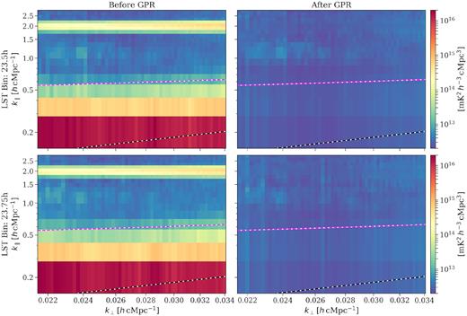
Cylindrically averaged Stokes I power spectra P(k⊥, k∥) of combined power spectra of eight nights per LST bin before (left-hand panels) and after (right-hand panels) foreground removal with GPR. Top and bottom panels correspond to LST:23.5 and LST:23.75 h, respectively. The black dashed line corresponds to the instrumental horizon, and the purple dashed line corresponds to horizon buffer accounting for the window function.
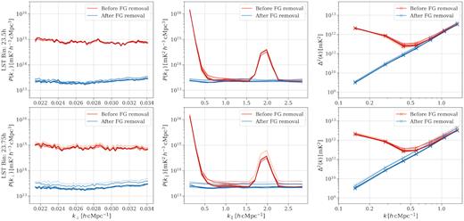
Stokes I power spectra before (red) and after (blue) foreground removal of different time-slices used in the analyses. The left-hand panels show P(k⊥), which is the average of P(k⊥, k∥) along the k∥ axis. The middle panels show P(k∥), which is the average of P(k⊥, k∥) along the k⊥ axis. The right-hand panels show the spherically averaged power spectra. Different colour shades represent different time-slices.
Fig. 6 shows the ratio between the residual Stokes I power spectrum after foreground removal (shown in the right-hand panels of Fig. 4) and the corresponding noise power spectrum for the two LST bins. We observe that the ratio is approximately flat except for the faint RFI structure, as mentioned previously. For the LST:23.5-h bin, the ratio has a median of ∼1.01 and a MAD of ∼0.08. For the LST:23.75-h bin, the median ∼ 1.00 and MAD ∼ 0.08. This shows that Stokes I residuals are almost entirely noise dominated for both LST bins.
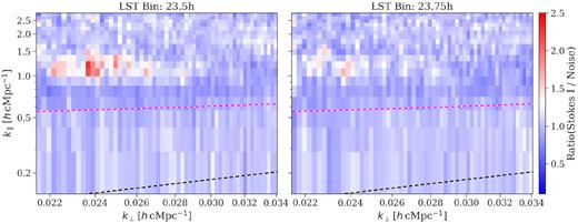
The ratio of residual Stokes I power spectrum after foreground removal and the estimated noise power spectrum. The left- and right-hand panels correspond to LST:23.5 and LST:23.75 h, respectively. The black dashed line corresponds to the instrumental horizon, and the purple dashed line corresponds to horizon buffer accounting for the window function.
6.2 Cross-coherence between nights
We use residual Stokes I data to compute cross-coherence between different pairs of time-slices corresponding to different nights within an LST bin. We calculate the mean cross-coherence in three regions (as in Mertens et al. 2020):
the foreground region (k∥ < 0.6),
the subband ripple region (1.7 < k∥ < 2.36),
The ‘EoR window’ (|$0.6\lt k_{\parallel }\lt 1.7 \& k_{\parallel }\gt 2.3$|).
Fig. 7 shows the mean cross-coherence between different pairs of nights for a given LST bin for these three regions of (k⊥, k∥) space. Foreground region shows a mean coherence of ∼0.2–0.3 for the two LST bins. It is possible that the observed correlation originates due to the sky emission outside the FoV (|$\sim \! 120{^\circ }$|) used in the analysis, and remained unsubtracted even after GPR foreground removal. The subband ripple region, on the other hand, shows a low coherence Ci, j ∼ 0.01–0.02, suggesting that the ripple is mitigated reasonably well with the strategy we have employed. However, it may become more severe as we integrate more data in future analyses. The coherence Ci, j < 0.01 of most pairs in the EoR window; however, time-slice pairs (3,4), (3,5), and (4,5) show slightly higher coherence (Ci, j ∼ 0.01). These time-slices are affected more by the faint RFI structure that also affects the coherence in the EoR window.
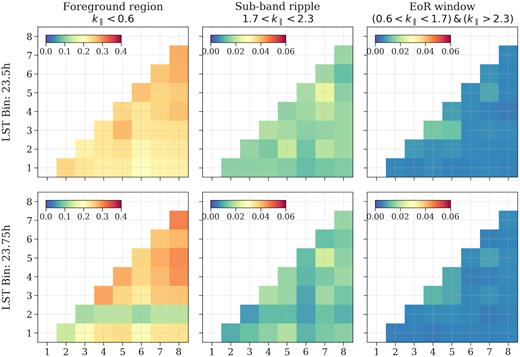
Mean cross-coherence of different pairs of time-slices in various regions (different columns) of (k⊥, k∥) space. The three columns (left- to right-hand side) correspond to the foreground, subband ripple, and EoR window regions, respectively. The eight different time-slices in a given LST bin are numbered from 1 to 8. Top and bottom panels correspond to LST:23.5- and LST:23.75-h bins, respectively.
To understand the RFI structure better, we also compute the mean cross-coherence in the region |$1.0\lt k_{\parallel }\lt {1.5} \ \ {\rm and} \ k_{\perp }\lt 0.026$|, which was affected the most by the RFI structure. For this case, we compute the coherence between all time-slices across the two LST bins. Fig. 8 shows the corner plot of the coherence of the RFI-affected region of (k⊥, k∥) space. We find that combinations of time-slice pairs between (5–10) show relatively higher coherence (Ci, j ∼ 0.02–0.04) and these nights were observed over 12 d. Note that time-slice pairs (2i − 1, 2i) belong to same ith observing night (except (3,4)). Any sky emission would decorrelate over short periods (e.g. between the two LST bins), whereas an RFI source on the ground would still be correlated over longer times. This provides additional evidence that the structure is transient and persisted over a span of two to three weeks, possibly some temporary source of local RFI. Other pairs show smaller correlations, similar to correlation levels in the EoR window.
![Mean cross-coherence of different pairs of time-slices in the region in (k⊥, k∥) space surrounding the RFI structure. Odd-numbered time-slices correspond to the LST:23.5-h bin and even-numbered time-slices correspond to the LST:23.75-h bin (respectively). Time-slice pairs (2i − 1, 2i) where i ∈ [1, 8] belong to the same night except pair (3,4). Time-slices are arranged in the order of increasing observing date.](https://oup.silverchair-cdn.com/oup/backfile/Content_public/Journal/mnras/499/3/10.1093_mnras_staa3093/1/m_staa3093fig8.jpeg?Expires=1750350415&Signature=Cij234fV-BfBWJDmR0jauC5DMxbyiClv0zwWTLAQ9R0rgn0WHVQ18rcfVDpwZxjMC6Pqb46LoI3K0cQzeShJSI37L-zvbK2RQ6SpKW2GsE701pI0JMOIhWkzuMlyDIU0xwFjhnv7JpDAuMnZQATmheJQuSkCWDrcAvIfQIdYpjwqpWH~X6YAW6pXgYtENgUR88ekpDVwHkstTlK7RTy4nfy5SMuaPgSY7j4YK55H4-JipWRfLnhcnNWK6o283ldu6IGYwTpxI5hS6Z5m-eDGD5KLWLoIBQBIwyzPoTH~ndLc-hn1txzp5XYudGkLUs4VB-4ByA4nemphwDKLGgpvtA__&Key-Pair-Id=APKAIE5G5CRDK6RD3PGA)
Mean cross-coherence of different pairs of time-slices in the region in (k⊥, k∥) space surrounding the RFI structure. Odd-numbered time-slices correspond to the LST:23.5-h bin and even-numbered time-slices correspond to the LST:23.75-h bin (respectively). Time-slice pairs (2i − 1, 2i) where i ∈ [1, 8] belong to the same night except pair (3,4). Time-slices are arranged in the order of increasing observing date.
6.3 Power spectra of combined time-slices
We used the procedure described in Section 4.1 to combine different nights/time-slices in a given LST bin. The GPR foreground removal is performed on intermediate data sets obtained after adding time-slice on by one. Fig. 9 shows the spectral variance, cylindrical power spectra averaged over all k⊥, and spherically averaged power spectra of residual Stokes I data in intermediate combined data sets. As expected, variance and power spectra scale down in amplitude with integration time as we add more data to a given LST bin. Additionally, power spectra appear to be dominated by noise and devoid of any obvious, coherent structures that may emerge after integrating more time-slices. There are several frequency channels with slightly higher covariance, which is probably due to slightly higher levels of RFI flagging than the rest. Two channels on the higher frequency end show relatively lower variance, which cannot be explained by higher RFI fraction. We are investigating the cause of the low variance of these two channels, and how it impacts the analysis and results.
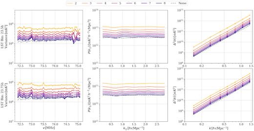
Various statistics for residual Stokes I of intermediate data sets with the increasing number of time-slice integration. From the left- to right-hand side: variance, cylindrical power spectrum averaged over all k⊥ modes, and spherically averaged power spectrum. Top and bottom panels correspond to LST:23.5- and LST:23.75-h bins. Different colours correspond to the number of nights averaged (in increasing order from yellow to purple) in order of observing dates. The dashed grey line shows the thermal noise corresponding to eight time-slices combined in a single LST bin. Note that spherically averaged power spherical power spectra shown here are not corrected for the noise bias.
6.4 Noise bias-corrected power spectrum
The uncertainty value |$\Delta _{21,\text{err}}^2$| on the power spectrum |$\Delta _{21}^2$| includes the sample variance (due to the number of individual uv-cells and effective FoV) and a contribution from the uncertainty on the hyperparameters of the GP model used in the analysis. However, the inferred values of most hyperparameters of the GP model are well constrained with very small uncertainty levels (|$\lesssim \! 1{{\ \rm per\ cent}}$| as shown in Table 2), except for the 21-cm signal, suggesting that the GPR error contribution to the final uncertainty on the power spectrum can be ignored. Similar findings have been reported in the application of GPR on LOFAR-HBA data (Mertens et al. 2020) as well as on HERA data (Ghosh et al. 2020).
We also combine |$\Delta _{21}^2$| for the two LST bins incoherently using inverse variance weighting to obtain incoherently averaged power spectrum. These noise bias-corrected power spectra for the two LST bins, and the incoherently averaged power spectrum are shown in Fig. 10. After 2 h (8 × 15 min) of integration per LST bin, we obtain a 2σ upper limit of |$\Delta _{21}^2 \lt (8139~\text{mK})^2$| at |$k = 0.144~h\, \text{cMpc}^{-1}$| for LST:23.5-h bin, and |$\Delta _{21}^2 \lt (8549~\text{mK})^2$| at |$k = 0.144~h\, \text{cMpc}^{-1}$| for LST:23.75-h bin, respectively, in the redshift range z = 17.9–18.6. The incoherently averaged power spectrum yields |$\Delta _{21}^2 \lt (7388~\text{mK})^2$| at |$k = 0.144~h\, \text{cMpc}^{-1}$|. We observe that the upper limit scales down by a factor of 1.1, compared to the expected factor of |$\sqrt{2}$|. We also observed that the power spectra are dominated by noise at all k-scales probed by ACE.
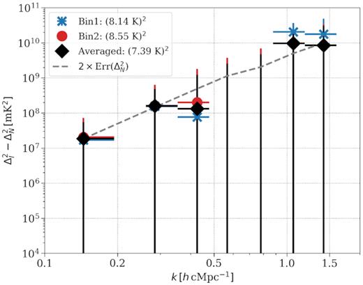
Noise bias-corrected power spectra |$\Delta _{21}^2$| for the two LST bins (‘crosses’ correspond to the LST:23.5-h bin and ‘circles’ correspond to the LST:23.5-h bin). The incoherently averaged power spectrum is shown using diamond markers. The dashed line shows the error on the noise power spectrum, which corresponds to the theoretically achievable 2σ upper limit in 2 h of coherent averaging. The x-error bars represent the range of k bins and y-error bars represent 2σ errors on the power spectra.
7 SUMMARY AND FUTURE WORK
In this work, we described the ACE program motivated by the reported detection of the deep absorption feature in sky-averaged spectrum of the 21-cm signal during CD by the EDGES collaboration (Bowman et al. 2018). Main results of the paper are summarized as follows:
We demonstrate the successful end-to-end application of the ACE data-processing pipeline (which is adapted from LOFAR-EoR data processing pipeline) to ACE data, starting from pre-processing and calibration to power spectrum estimation after foreground removal.
We observe that the ratio of noise estimates from the channel and time-differenced Stokes V visibilities varies between 1.0 and 1.2 for most time-slices in the two LST bins. The mean ratio per LST bin shows weak baseline dependence, which is possibly caused by residual Stokes I to V leakage. We use channel differenced Stokes V noise as an estimator of frequency uncorrelated noise and later for noise bias correction.
Residual power spectra reach the expected noise level to within 1 per cent. Cylindrically averaged Stokes I power spectra exhibit a faint structure between 0.1 < k∥ < 1.5 and k⊥ < 0.026. This structure appears to be transient (as shown by the cross-coherence test) and affects certain baselines. We suspect this structure is possibly caused by faint RFI that remained undetected by flagging strategy we have employed in the analysis. Combining multiple nights decreases the power as expected, and corresponding power spectra of combined data do not show any obvious coherent emission.
Even though the noise bias-corrected power spectrum is still dominated by noise, it is not regarded as a detection because the power levels within 2σ are two to three orders of magnitude higher than the expected signal and the power still decreases by adding more data. We thus obtain a 2σ upper limit of |$\Delta _{21}^2 \lt (8139~\text{mK})^2$| (or equivalently (8.14 K)2) and |$\Delta _{21}^2 \lt (8549~\text{mK})^2$| (or equivalently (8.55 K)2) at |$k = 0.144~h\, \text{cMpc}^{-1}$| for LST:23.5-h and LST:23.75-h bins, respectively. The incoherently averaged power spectrum yields |$\Delta _{21}^2 \lt (7388~\text{mK})^2$| (or equivalently (7.39 K)2) at the same k value. These limits correspond to the redshift range z = 17.9–18.6.
Although the upper limits are still at least two orders of magnitude higher than signals predicted by simulations, adding more data in future will allow us to improve these limits and possibly exclude or constrain various astrophysical models that may explain the 21-cm signal from the CD.
7.1 Future outlook and forecast
In this work, we demonstrated the successful application of the new ACE data-processing pipeline and effectively reaching the expected noise levels. However, most of the steps used in the analysis are still fairly rudimentary and require improvements. In the future, we plan to improve the processing and analysis by improving several aspects of the ACE data-processing pipeline as follows:
Improving DI calibration of the data by including a detailed sky-model (compact sources and large-scale diffuse emission). It will also allow a better direction subtraction/peeling of bright sources, Cas A and Cyg A, to mitigate residuals post-subtraction.
The subband ripple is a dominant systematic in ACE data. Currently, we use a covariance model in GPR (along with PCA) to mitigate it, which is suboptimal. The subband ripple is a multiplicative effect as it is caused by the bandpass shape of the polyphase filterbank. We are exploring methods and strategies to mitigate the subband ripple during the calibration step rather than during the post-imaging steps.
The RFI removal strategy used by aoflagger in the current analysis is based on LOFAR-LBA RFI mitigation strategy, which may be suboptimal for noisier ACE data. We plan to improve the current RFI-mitigation strategy to work on ACE data optimally. We also plan to use a near-field imaging technique to pinpoint whether the cause of the faint RFI is due to sources on the ground. In addition to this, we plan to alternatively explore RFI mitigation techniques that use polarization information and directional statistics of RFI for RFI detection and removal (Yatawatta 2020).
Our current analysis is based on coherently averaging data in a given LST range. In the future, we plan to widen the LST range using map-making methods based on spherical harmonics techniques to achieve a lower noise floor.
Low-frequency wide-field observations are more prone to effects from polarization leakage and the ionosphere. We plan to study the effect of polarization leakage and the ionosphere in ACE observations and mitigate them if required.
Incorporating the improvements as mentioned above to the data processing pipeline allows us to decrease the power spectrum levels further. Assuming that foregrounds and systematics are optimally mitigated/removed, a power spectrum sensitivity of |$\Delta _{21}^2 \lt (1\, \textrm {K})^2$| may be reached in 150 h of integration and even lower levels with the 500 h of data in hand. This sub-Kelvin sensitivity is already at the level of some predictions of the 21-cm fluctuations during the CD (Fialkov et al. 2018; Fialkov & Barkana 2019).
ACKNOWLEDGEMENTS
BKG and LVEK acknowledge the financial support from a NOVA cross-network grant. BKG acknowledges the National Science Foundation grant AST-1836019. FGM, MK, and AS acknowledge support from a SKA-NL roadmap grant from the Dutch Ministry of OCW. This work was supported in part by ERC grant 247295 ‘AARTFAAC’ to RAMJW. LOFAR, the Low Frequency Array designed and constructed by ASTRON, has facilities in several countries, that are owned by various parties (each with their own funding sources), and that are collectively operated by the International LOFAR Telescope (ILT) foundation under a joint scientific policy. This research made use of publicly available software developed for LOFAR and AARTFAAC telescopes. Here is a list of software packages used in the analysis: aartfaac2ms (https://github.com/aroffringa/aartfaac2ms), aoflagger (https://gitlab.com/aroffringa/aoflagger), dppp (https://github.com/lofar-astron/DP3), wsclean (https://gitlab.com/aroffringa/wsclean), and GPR foreground removal code (https://gitlab.com/flomertens/ps_eor). The analysis also relies on the python programming language (https://www.python.org) and several publicly available python software modules: astropy (https://www.astropy.org; The Astropy Collaboration 2013), gpy (https://github.com/SheffieldML/GPy), emcee (https://emcee.readthedocs.io/en/stable/; Foreman-Mackey et al. 2013), matplotlib (https://matplotlib.org/), scipy (https://www.scipy.org/), and numpy (https://numpy.org/).
DATA AVAILABILITY
The data underlying this paper will be shared on reasonable request to the corresponding author.
Footnotes
LOFAR proposal ID: LT10_006. Investigators: Gehlot and Koopmans.
AARTFAAC-LBA (unlike HBA) does not beam-form to track; it only points to the instantaneous zenith direction per integration time in drift-scan mode. During preprocessing, the drift-scan data for a long observational run are split into 15-min observation blocks and rephased. The phase centre for each block follows a constant declination point that passes through the zenith half-way during the 15-min run. We refer to this strategy as the ’semi drift-scan’ mode.
LBA dipoles are dual-polarization (X–Y) dipoles optimized to operate between 30 and 80 MHz.
HBA tiles consist of 16 dual-polarization dipoles arranged in a 4 × 4 grid, which are analogue beam-formed to produce a single tile beam. HBA tiles are optimized to operate between 110 and 240 MHz.
Current LOFAR-LBA dipole beam models are based on electro-magnetic (EM) simulations of the LOFAR-LBA dipoles (private communication with LOFAR Radio Observatory).
The ‘Hann’ window is defined as
where 0 ≤ n ≤ M − 1.
AARTFAAC team via private communication.
