The completed SDSS-IV extended Baryon Oscillation Spectroscopic Survey: BAO and RSD measurements from the anisotropic power spectrum of the quasar sample between redshift 0.8 and 2.2

Effective area and number of quasars used in the clustering analyses.

Cap	NGC	SGC	Total
Weighted area (deg²)	2860	1839	4699
Quasars used 0.8 < z < 2.2	\|$218\, 209$\|	\|$125\, 499$\|	\|$343\, 708$\|

Table 1.

Effective area and number of quasars used in the clustering analyses.

Cap	NGC	SGC	Total
Weighted area (deg²)	2860	1839	4699
Quasars used 0.8 < z < 2.2	\|$218\, 209$\|	\|$125\, 499$\|	\|$343\, 708$\|

2.2 Estimation of the power spectrum and extraction of cosmological parameters

We study the quasar survey through its power spectrum:

$$\begin{eqnarray*} P(\bf k) = (2\pi)^3 \delta ^D({\bf k} + {\bf k^\prime })\langle \delta (\bf k)\delta (\bf k^\prime) \rangle , \end{eqnarray*}$$

(3)

where δ(k) is the density perturbation field and δ^D is the Dirac distribution.

For the calculation of the power spectrum, we use the method of Yamamoto et al. (2006). First, we construct a weighted object over-density field, F(r) (Feldman et al. 1994), at each position r,

$$\begin{eqnarray*} F({\bf r})=n_\mathrm{ q}({\bf r})-\alpha n_{\mathrm{ r}}({\bf r}), \end{eqnarray*}$$

(4)

where n_q is the number density field for the quasar catalogue and n_r is the number density of objects in the random catalogue described in Section 2.1. Both are including the weights described in equations (1) and (2). The random field is scaled by |$\alpha =\frac{\sum _i w_{\mathrm{ q},i}}{\sum _i w_{\mathrm{ r},i}}$| to ensure that the mean weighted densities of data and random are the same. Then, following Bianchi et al. (2015), the power spectrum multipoles are given by:

$$\begin{eqnarray*} P_\ell (k)=\frac{2\ell +1}{I}\int \frac{d\Omega _k}{4\pi }\left[F_0({\bf k})F_\ell ({-\bf k})-P^{\rm noise}_0(k)\right], \end{eqnarray*}$$

(5)

where I is the normalization of the power spectrum, defined as

$$\begin{eqnarray*} I=\alpha \sum _{i=1}^{N_r} w_{\mathrm{ r},i}n_{\mathrm{ q},i}, \end{eqnarray*}$$

(6)

and |${\cal L}_\ell$| is the ℓth order Legendre polynomial. Ω_k is the solid angle in Fourier Space, and F_ℓ(k) is defined as

$$\begin{eqnarray*} F_{\ell }({\bf k}) = \int d^{3} r F({\bf r}) {\cal L}_\ell (\hat{\bf k} \cdot \hat{\bf r}) e^{i {\bf k} \cdot {\bf r}}. \end{eqnarray*}$$

(7)

The shot noise component, |$P^{\rm noise}_\ell (k)$|⁠, is expressed as

$$\begin{eqnarray*} P^{\rm noise}_0(k)=\sum _{i}w^2_{\mathrm{ q},i} + \alpha ^2\sum _{i}w^2_{\mathrm{ r},i}. \end{eqnarray*}$$

(8)

In practice, we use the nbodykit package (Hand et al. 2018) to calculate the power spectrum multipoles using the method of Hand et al. (2017). First, the weighted density field is mapped on to a cubic grid using the Triangular Shaped Cloud interpolation method. Each cap is enclosed in a box of dimensions |$L_{\mathrm{ box}}=[3100,6500,2700]\, \mathrm{h}^{-1}\mathrm{Mpc}$|⁠. The cell size is chosen to be |$7\, \mathrm{h}^{-1}\mathrm{Mpc}$|⁠, yielding a Nyquist frequency of |$k_{\rm Nyq}=0.449\, \mathrm{h}\cdot \mathrm{Mpc}^{-1}$| well above the maximum wavenumber of our analysis (⁠|$k_{\rm max}=0.3\, \mathrm{h}\cdot \mathrm{Mpc}^{-1}$|⁠). Then, the F_ℓ(k) term can be computed with a Fast Fourier Transform, and the interlacing technique is used to reduce the effect of aliasing (Sefusatti et al. 2016). In the top panel of Fig. 1, we show the impact of photometric weights in the calculation of the power spectrum for the South Galactic Cap, which is known to be the most affected by photometric systematics, as demonstrated in Zarrouk et al. (2018). We observe that the correction brought by the photometric weight changes the multipoles on scales |$k\lt 0.05\, \mathrm{h}\cdot \mathrm{Mpc}^{-1}$|⁠. In Section 4.3.1, we use the approximate mocks to evaluate the impact of applying and correcting for systematic effects.

Figure 1.

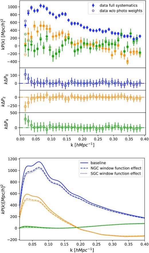
Top panel: Power spectrum of the SGC data with all weights applied (solid circle) or without the photometric weight (open circle); the effect on the NGC (not shown here) is smaller. Represented are the multipoles of the power spectrum: monopole (blue), quadrupole (red), and hexadecapole (green). Lower panel: Impact of the NGC (dashed line) and SGC (dotted line) window function on the power spectrum multipoles of a baseline power spectrum (solid line, same colour scheme as in the top panel).

The observed density of quasars is measured according to a survey-specific selection function that must be folded into the model. Following the method described in Beutler et al. (2016), the selection function multipoles are determined in configuration space from the weighted number of pairs in the ‘random’ catalogue as

$$\begin{eqnarray*} W_\ell (r) \propto \sum _{\mu }\sum _{x_1}\sum _{x_2}RR(r,\mu)L_\ell (\mu), \end{eqnarray*}$$

(9)

with RR(r, μ) being the random–random pair counts in bins of separation r and μ, where μ is defined as the cosine of the angle between the line of sight and the line connecting the two objects of a pair. As proposed in de Mattia & Ruhlmann-Kleider (2019), the window function is normalized by the quantityI (equation 6), in order to be consistent with the estimator of the power spectrum, which ensures that the model fitting is independent of the choice of normalization. The effect of the window function on the power spectrum multipoles, using the power spectrum model described in Section 4.1, is shown in the bottom panel of Fig. 1. Small differences between the two galactic caps are observed and arise from the difference in angular size and shape of their respective footprints (the SGC footprint is indeed smaller and patchier).

As a single line of sight is used for each galaxy pair, wide-angle effects may arise and are taken into account using the formalism described in Beutler, Castorina & Zhang (2019), which consists of expanding the survey window function in s/d, the ratio of pair separation to the comoving distance from the observer.

In the analyses performed hereafter, we assume a fiducial cosmology to convert redshifts to distances along the line of sight and to calculate a power spectrum template:

$$\begin{eqnarray*} h &=& 0.676, \, \, \Omega _{\mathrm{ m}} = 0.31, \, \, \Omega _{\Lambda } = 0.69,\nonumber \\ \Omega _{b}h^{2} &=& 0.022, \, \, \sigma _{8} = 0.80. \end{eqnarray*}$$

(10)

To fit to the data, we allow for variations of the dilation scales along (⁠|$\alpha _{\parallel }$|⁠) and perpendicular (α_⊥) to the line of sight, following the test proposed by Alcock & Paczynski (1979). Changing the dilation scales in configuration space is equivalent to setting |$k^{\prime }_{\parallel }=k_{\parallel }/\alpha _{\parallel }$| and |$k^{\prime }_{\perp }=k_{\perp }/\alpha _{\perp }$|⁠. This change of scales corresponds to the transformation from (k, μ) to (k^′, μ^′) where

$$\begin{eqnarray*} k^{\prime }&=&\frac{k}{\alpha _{\perp }}\left[1+\mu ^2\left(\frac{1}{F^2}-1\right)\right]^{1/2}\nonumber \\ \mu ^{\prime }&=&\frac{\mu }{F\left[1+\mu ^2\left(\frac{1}{F^2}-1\right)\right]^{-1/2}}, \end{eqnarray*}$$

(11)

where F = |$\alpha _{\parallel }$|/α_⊥.

Provided the constraints on |$\alpha _{\parallel }$| and α_⊥ come only from the BAO location, these quantities are related to the Hubble distance D_H ≡ c/H(z), where H(z) is Hubble expansion, and to the transverse diameter distance D_M(z) independently of the choice of fiducial cosmology through the following expressions:

$$\begin{eqnarray*} \alpha _{\parallel }=\frac{D_{\rm H}(z)/r_{\rm drag}}{D_{\rm H}^{\rm fid}(z)/r_{\rm drag}^{\rm fid}},\qquad \alpha _{\perp }=\frac{D_{\rm M}(z)/r_{\rm drag}}{D_{\rm M}^{\rm fid}(z)/r_{\rm drag}^{\rm fid}}, \end{eqnarray*}$$

(12)

where the quantities with the superscript ‘fid’ are determined within the fiducial cosmology and r_drag is the comoving sound horizon at z = z_drag, where z_drag is the redshift at which the baryon-drag optical depth equals unity (Hu & Sugiyama 1995). In the case of spherically averaged clustering measurements, the analysis is sensitive to an isotropic dilation scale, α_iso, that can be expressed as

$$\begin{eqnarray*} \alpha _{\mathrm{iso}}=\frac{D_{\rm V}(z)/r_{\rm drag}}{D_{\rm V}^{\rm fid}(z)/r_{\rm drag}^{\rm fid}}, \end{eqnarray*}$$

(13)

where D_V(z) corresponds to the spherically averaged BAO distance that we can link to the other cosmological parameters through the relation (Eisenstein et al. 2005; Ross, Percival & Manera 2015):

$$\begin{eqnarray*} D_{\rm V}(z)=\left[czD_{\rm H}(z)D_{\rm M}(z)\right]^{1/3}\!. \end{eqnarray*}$$

(14)

The linear growth rate of structures, f, is determined from a ‘Full-Shape’ fit of the power spectrum multipoles. In practice, the non-linear power spectrum is calculated assuming a linear power spectrum of known normalization, which is proportional to σ₈, the amplitude of matter perturbations below scales of |$8\, \mathrm{h}^{-1}\mathrm{Mpc}$|⁠. In linear theory, f and σ₈ are completely degenerate (Percival & White 2009), and hence, our measurement is sensitive to the product, f(z)σ₈(z), at the effective redshift of the survey.

The definition of the effective redshift adopted in this analysis is

$$\begin{eqnarray*} z_{\rm eff}=\frac{\sum _i \sum _j w_i w_j (z_i+z_j)/2}{\sum _i \sum _j w_i w_j }=1.480\pm 0.001, \end{eqnarray*}$$

(15)

where the sums are restricted to separations between 25 and |$120\, \mathrm{h}^{-1}\mathrm{Mpc}$|⁠, as this corresponds to the scales over which the fits are performed in configuration space. The error quoted is the statistical error on the unweighted redshift distribution.

2.2.1 Parameter estimation

For both the BAO analysis (Section 3) and the full-shape RSD analysis (Section 4), the best-fitting model parameter values are obtained by finding the point in parameter space that maximizes the likelihood function,

$$\begin{eqnarray*} L \propto e^{-\chi ^2/2}, \end{eqnarray*}$$

(16)

with the quantity χ² defined by

$$\begin{eqnarray*} \chi ^2=(P_{\rm meas}-P_{\rm model})^t W(P_{\rm meas}-P_{\rm model}). \end{eqnarray*}$$

(17)

P_meas is the data vector of the power spectrum multipoles measurement in intervals of wavenumber k, and P_model is the corresponding vector for the model. In this expression, W is the inverse of the covariance matrix computed from EZmocks, described in Section 2.3.1, which we correct for the finite number of mocks following Hartlap, Simon & Schneider (2007):

$$\begin{eqnarray*} W = \frac{N-n-2}{N-1}C^{-1}, \end{eqnarray*}$$

(18)

where N is the total number of mocks, and n is the number of data points. Furthermore, due to the uncertainty in the covariance matrix, a correction on the variance of the fit parameters is applied, following Percival et al. (2014). The total χ² combines the NGC and the SGC with a common set of α_⊥, |$\alpha _{\parallel }$| and fσ₈ parameters (or just α_⊥ and |$\alpha _{\parallel }$| for the BAO-only analysis). The nuisance and bias parameters are allowed to differ for the two galactic caps. We determine the covariance matrices independently in each cap assuming that there is no cross-correlation between the two caps. Therefore, the number of points n to be used in equation (18) corresponds to the number of data points in a single cap (i.e. 84 over the full k-range, including all even multipoles up to ℓ = 4).

We use, for the final result of the Full-Shape RSD analysis, the likelihood function defined in equation (16) to produce Monte Carlo Markov Chains with the emcee package (Foreman-Mackey et al. 2013). We check the convergence of the chains with the Gelman–Rubin convergence test requiring R < 0.01. The χ² minimization is performed using the MINUIT² program libraries. In this case, parameter errors are determined from finding the Δχ² = 1 abscissa along the 1D χ² profile for each parameter. After ensuring that the errors of both techniques are compatible, we apply this frequentist method for all the results of this paper concerning mocks as well as the various tests done on the data as it is much faster (usually, the fit outperforms the MCMC running by a factor of 1000 in terms of CPU time).

2.3 Mocks

We present, in the following, the two sets of mocks that we use: the approximate EZmocks are used to estimate the observational systematic errors and the computation of the covariance matrix, and the mocks created from N-body simulations are used to derive the modelling systematic errors.

2.3.1 EZmocks

To determine the covariance matrix to be used in the fits to the data and to test our analysis pipeline, we use a set of 1000 approximate light-cone mock catalogues that are extensively described in Zhao et al. (2020). These mocks, dubbed EZmocks, are made using the framework of the Effective Zel’dovich approximation developed in Chuang et al. (2015). The number of mocks (i.e. 1000) is chosen such that the correction given in equation (18) is below 10 per cent. The simulation box is a cube with a comoving side length of |$5\, \mathrm{h}^{-1}\mathrm{Gpc}$|⁠. The ΛCDM cosmology assumed when creating the EZmocks has the following parameters:

$$\begin{eqnarray*} h &=& 0.6777, \, \, \Omega _{\mathrm{ m}} = 0.307115, \, \, \Omega _{\Lambda } = 0.692885,\nonumber \\ \Omega _{\mathrm{ b}} &=& 0.048206, \, \, \sigma _{8} = 0.8225, \, \, n_\mathrm{ s}=0.9611 . \end{eqnarray*}$$

(19)

For the quasars, the light-cone mocks are built from seven simulation snapshots, and the clustering signal in the mocks is tuned to match the one of the final DR16 quasar catalogues (see Fig. 2). At the scale of the second BAO wiggle, |$k\sim 0.14 \, \mathrm{h}\cdot \mathrm{Mpc}^{-1}$|⁠, the data are in excess of power compared to the EZmocks. That is due to a stronger BAO signal in the data. The EZmocks are mocks generated with a fast technique, which is a good approximation of an N-body simulation mock at large scales, but may fail to reproduce the non-linear gravity interactions at small scales accurately. This might explain the mild lack of power on the monopole of the EZmocks corrected for shot noise for both caps at |$k\gt 0.25 \, \mathrm{h}\cdot \mathrm{Mpc}^{-1}$|⁠.

Figure 2.

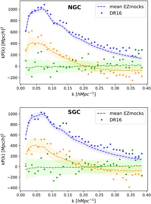
Multipoles of the power spectrum measured with the DR16 eBOSS quasar sample (dots) compared to the EZmocks (dashed line). The standard deviation of the mocks is indicated by the shaded area. The NGC and the SGC are shown in the top and bottom panels, respectively. The monopole is shown in blue and the shot noise contribution is subtracted, the quadrupole in red, and the hexadecapole in green.

In practice, it is the monopole not corrected for shot noise of the EZmocks that is used in the determination of the covariance matrix. For this quantity, we see that the EZmocks tend to overestimate the monopole by 3 per cent, and this will result in a conservative overestimation of the errors on the fit parameters by the same amount.

Furthermore, the power spectrum monopole for the quasar sample is increasingly dominated by shot noise as k increases. As the weighted number of objects in the mocks are matched to the data by construction, the shot noise terms are the same and the impact of the lack of power at small scales is reduced. Quantifying the residual impact this has on the measurement of the cosmological parameters is addressed in the studies of systematic effects in the next sections.

Mocks are also used to estimate the impact of systematic effects present in the data. To do so, the approximate EZmocks are modified to reflect the effects induced by observational conditions. First, mock ‘data’ catalogues are created by taking mock quasars in the redshift range of 0.75 < z < 2.25. The mock catalogues are downsampled by an amount that allows to match the radial selection function of the data at the end of the procedure. Then, contaminants (stars, galaxies, and ‘legacy’ quasars), which were known before the quasar survey and that fulfilled the quasar target selection conditions, are added to this catalogue. The fibre assignment algorithm (based on nbodykit; Hand et al. 2018) is run on this set of targets using the plate geometry of the DR16 data. As in the data, objects that could not receive a fibre are treated by up-weighting the objects in the collision group that did receive a fibre. The effects of the imaging conditions are modelled by varying the number of targets according to the weight maps measured in the data. We use the spectroscopic success rate as a function of the identification number of the spectrograph fibre measured in the data as well as the plate signal-to-noise ratio to randomly remove objects. As a consequence, the objects in the mock catalogues receive a weight to cope for the spectroscopic success rate variations, as was described for the data catalogues.

2.3.2 OuterRim mocks and the quasar mock challenge

To test the model adopted for the power spectrum, we compare it against accurate mock catalogues of known cosmological parameters. For this purpose, we have performed a quasar mock challenge, which is described in details in Smith et al. (2020). We refer the reader to this article, and we briefly summarize the content and give the results here. The mocks are built from one snapshot (z = 1.433) of the OuterRim N-body simulations (Habib et al. 2016) that was available at the beginning of this work. Non-linear effects are mildly increasing with time; therefore, the tests of the model are performed conservatively since the effective redshift of the DR16 quasar sample corresponds to earlier times. The OuterRim simulation covers a cubic box of length |$L=3\, \mathrm{h}^{-1}\mathrm{Gpc}$| with periodic boundary conditions and uses 10240³ dark matter particles. The mass of each particle in the simulation is hence |$m_p = 1.85 \times 10^9\, {\rm M_\odot }h^{-1}$| and dark matter haloes are detected using a Friends-of-Friends algorithm. Initial conditions are calculated at z = 200 in the Zel’dovich approximation using the cosmological parameters:

$$\begin{eqnarray*} h &=& 0.71, \, \, \Omega _{\mathrm{cdm}}h^{2} = 0.1109, \, \, \Omega _{\Lambda } = 0.735,\nonumber \\ \Omega _{\mathrm{ b}}h^{2} &=& 0.02258, \, \, \sigma _{8} = 0.80, \, \, n_\mathrm{ s}=0.963, \end{eqnarray*}$$

(20)

which are consistent with WMAP7 (Komatsu et al. 2011). To populate dark matter haloes with quasars, we consider various Halo Occupation Distribution (HOD) models. An HOD describes the probability that a halo of a given mass contains central or satellite quasars. Central quasars are placed at the centre of the halo, while satellites are placed either according to an NFW profile (Navarro, Frenk & White 1996) or by drawing a particle from a |$1{{\ \rm per\ cent}}$| subsample of the particles belonging to the halo. The list of HOD parameters can be found in Smith et al. (2020). For each HOD model, we generate 100 random realizations. We also reproduce the effect of redshift uncertainties, which are due to broad emission lines in the quasar spectra, and have been shown to be the leading effect, which impacts the recovery of cosmological parameters (Zarrouk et al. 2018). Three redshift-smearing prescriptions were applied: no redshift smearing, Gaussian smearing, and a realistic smearing case with non-Gaussian tails. A fourth set of mocks has been created starting from the realistic smearing case and assigning |$1.5{{\ \rm per\ cent}}$| of objects with a catastrophic redshift. We use these ‘non-blind’ mocks to tune the functional form of the damping term that enters our model of the power spectrum (see Section 4.1), which plays a leading role at small scales.

In a second stage, Smith et al. (2020) implemented the rescaling technique described in Mead & Peacock (2014) (itself based on the work of Angulo & White 2010) to create ‘blind’ mocks, whose the true cosmology was revealed only at the end of the analysis. For this part of the mock challenge, two snapshots (z = 1.376 and z = 1.494) of the OuterRim N-body simulations have been rescaled to eight different cosmologies at z = 1.433 and for three types of HOD. No modifications to the models were undertaken after the cosmologies were un-blinded.

3 BAO ANALYSIS

In this section, we present the BAO-only analysis by first explaining the model, and then we present the results and the systematic tests performed.

3.1 Model

The modelling of the power spectrum for extracting the dilation scales parallel and perpendicular to the line of sight is based on the method described in Kirkby et al. (2013). In this method, the 2-point correlation function, which is the Fourier transform of the power spectrum, is decomposed into a ‘smooth’ term that characterizes the broad-band shape and into a ‘peak’ term representing the BAO wiggle part of the power spectrum. In the fiducial analysis, the smooth term is not affected by the dilation scaling but in the analysis named ‘smooth-term coupling’, we apply the dilation to both terms. The Fourier transform of these two terms, P_sm(k, μ) and P_peak(k, μ), is used to model the measured power spectrum through:

$$\begin{eqnarray*} P(k,\mu)=\left[P_{\rm sm}(k,\mu)+P_{\rm peak}(k,\mu)e^{-\Sigma _\mathrm{nl}k^2}\right]\frac{b^2(1+\beta \mu ^2)^2}{1+\frac{(k\mu \Sigma _s)^2}{2}}, \end{eqnarray*}$$

(21)

where Σ_nl is an anisotropic damping term of the BAO feature, b represents the linear bias of the quasars, β = f/b is linear enhancement of the power spectrum due to RSDs, and Σ_s is another damping term accounting for random velocities at small scales and redshift uncertainties. Given the low density of the quasar sample, the BAO reconstruction technique cannot be applied successfully as the matter field is not accurately sampled.

The power spectrum is then decomposed into Legendre multipoles (ℓ = 0, 2, 4), which are Fourier transformed to obtain the corresponding correlation functions. The window function is applied on the correlation function multipoles using the method presented in Beutler et al. (2016) and involves multipoles of the window function determined up to the ℓ = 8 order. A final Fourier transform is applied to the correlation function multipoles to obtain the window function convolved power spectrum multipoles.

Furthermore, to fit the broad-band part of the power spectrum, we add three polynomial terms to each multipole,

$$\begin{eqnarray*} P^f_\ell (k) = P_\ell (k)+\frac{a_{0,\ell }}{k}+a_{1,\ell }+a_{2,\ell }\cdot k, \end{eqnarray*}$$

(22)

where the a_{x, ℓ} are allowed to vary in the fitting procedure and are different for the two galactic caps.

The anisotropic non-linear damping of the BAO, Σ_nl, is modelled as

$$\begin{eqnarray*} \Sigma _{\mathrm{ nl}}=(1-\mu ^2)\Sigma _{\perp }^2/2+\mu ^2\Sigma _{\parallel }^2/2. \end{eqnarray*}$$

(23)

The values of the damping parameters |$\Sigma _{\parallel }$|⁠, Σ_⊥ and Σ_s are obtained from fitting the non-blind N-body mocks, described in Section 2.3.2. First, we used the set of mocks without redshift-smearing effects to determine |$\Sigma _{\parallel }$| and Σ_⊥. Then, we fix |$\Sigma _{\parallel }$| and Σ_⊥ to the obtained values and fit the mocks with realistic smearing to determine Σ_s. This procedure yields (in units of |$\, \mathrm{h}^{-1}\mathrm{Mpc}$|⁠):

$$\begin{eqnarray*} \Sigma _{\parallel }=8.5\pm 0.6\qquad \Sigma _{\perp }=2.9\pm 0.9 \qquad \Sigma _s=4.5\pm 1.1. \end{eqnarray*}$$

(24)

In Fig. 3, we present the BAO wiggle part of the power spectrum for the data and for the average of the EZmocks. Also plotted is the average of the 100 realizations from one set of OuterRim non-blind mocks (note that it is at a different cosmology than the EZmocks). The data show a clear detection of the BAO for both galactic caps, and the amplitude of the oscillation is found to be larger than in the EZmocks. The amplitude of the oscillation in the EZmocks is itself smaller than the expectation in the case of the Zel’dovich approximation.

Figure 3.

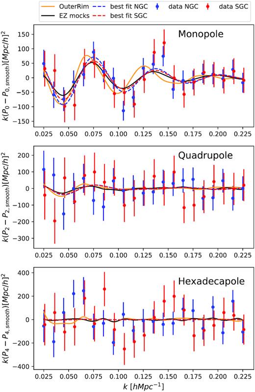
Comparison of the BAO wiggles in the power spectrum of the data and mocks. The dots represent the DR16 data, the dashed lines are the best fit, and the black line shows the mean of the NGC EZmocks. The green line shows the mean of one realization of the OuterRim mock challenge (mock3) with realistic smearing. For the latter, the BAO feature appears shifted as a consequence of their intrinsic cosmology being different.

For the fiducial analysis, the fit is performed over wave numbers |$k=[0.02, 0.23]\, \mathrm{h}\cdot \mathrm{Mpc}^{-1}$| that cover the first three visible BAO oscillations. We use 22 free parameters: the two dilation scale parameters, two bias parameters (one for each cap), and 18 broad-band terms (three for each cap and each multipole), with intervals of allowed variations of b = [0, 10] and |$\alpha _{\parallel }$|_{, ⊥} = [0.8, 1.2] that are large enough that boundaries are never hit. The three damping terms are fixed to |$[\Sigma _{\parallel }, \Sigma _{\perp } ,\Sigma _s]=[8,3,4]\, \mathrm{h}^{-1}\mathrm{Mpc}$| since letting them free in the fit may result in an artificial improvement of the statistical precision (Hinton, Howlett & Davis 2020).

We use the mock challenge (Smith et al. 2020) to determine the systematic error originating from the modelling of the BAO feature in the power spectrum multipoles. The analysis is performed on all sets of OuterRim mocks in the non-blind and blind challenges, which includes the effects of different cosmologies, redshift error prescriptions, and different HOD models. The systematic errors are found to be

$$\begin{eqnarray*} \Delta (\alpha _\parallel)\!\!\left.\right|_\mathrm{model}=0.0098 \quad \Delta (\alpha _\perp)\!\!\left.\right|_\mathrm{model}=0.0055 \end{eqnarray*}$$

(25)

and are obtained from the standard deviation (w.r.t. the expected value) of the non-blind ‘realistic smearing + catastrophic redshifts’ mocks added in quadrature with that of the blind mocks.

3.2 Results

We perform the BAO-only analysis of the monopole, quadrupole, and hexadecapole of the power spectrum measured from the QSO DR16 catalogue, as described in Section 3.1. The covariance matrix is computed from the 1000 EZmocks. Fig. 3 shows the best-fitting model (dashed lines) to the data (points) with NGC and SGC fitted simultaneously. The results obtained from the BAO analysis in Fourier Space are in terms of α:

$$\begin{eqnarray*} \alpha _\parallel =1.035 \pm 0.045 \qquad \alpha _\perp =1.017 \pm 0.029, \end{eqnarray*}$$

(26)

where the errors are statistical only. In this section, we estimate the systematic errors on this measurement using a series of tests performed on the EZmocks and we verify on the data that the choices made for the analysis do not bias the results.

3.2.1 Systematic tests

The results of systematic checks that were performed on the EZmocks are summarized in Table 2. For these studies, the reference dilation scales are taken from mock catalogues with all observational systematic effect applied and corrected for using the standard weighting scheme (see equation 1). The reference model has the window function (wf) applied and the smooth-term is decoupled from the BAO peak term. Changing the prescription for the window function or smooth-term coupling induces changes that are at maximum 0.7 per cent (central value averaged over 1000 mocks). The magnitude of the difference is in agreement with the modelling systematic error quoted from the mock challenge (see equation 25).

Table 2.

Average |$\alpha _{\parallel }$| and α_⊥ values obtained for the 1000 EZmocks under different type of systematic effects and methods (first four rows) and results obtained for data with different model prescriptions and different damping values (bottom two rows). The ‘no wf’ line stands for the analysis performed without taking into account the window function correction, the ‘coupled’ line shows the impact of coupling the sideband of the model, and the lines w_noz + w_sys and fibre collisions show the effect of the redshift failures + photometric systematics or the collisions of fibres, respectively.

Tests on EZmocks	\|$\alpha _{\parallel }$\|	α_⊥
Reference	0.9938 ± 0.0027	0.9959 ± 0.0019
No wf	Δ = 0.0007(2)	Δ = 0.0011(1)
Coupled	Δ = 0.0031(11)	Δ = 0.0021(6)
No wf, coupled	Δ = 0.0068(13)	Δ = 0.0040(7)
w_noz + w_sys	Δ = 0.00108(228)	Δ = 0.00138(156)
Fibre collisions	Δ = −0.00296(121)	Δ = −0.00026(92)

Tests on EZmocks	\|$\alpha _{\parallel }$\|	α_⊥
Reference	0.9938 ± 0.0027	0.9959 ± 0.0019
No wf	Δ = 0.0007(2)	Δ = 0.0011(1)
Coupled	Δ = 0.0031(11)	Δ = 0.0021(6)
No wf, coupled	Δ = 0.0068(13)	Δ = 0.0040(7)
w_noz + w_sys	Δ = 0.00108(228)	Δ = 0.00138(156)
Fibre collisions	Δ = −0.00296(121)	Δ = −0.00026(92)

Table 2.

Average |$\alpha _{\parallel }$| and α_⊥ values obtained for the 1000 EZmocks under different type of systematic effects and methods (first four rows) and results obtained for data with different model prescriptions and different damping values (bottom two rows). The ‘no wf’ line stands for the analysis performed without taking into account the window function correction, the ‘coupled’ line shows the impact of coupling the sideband of the model, and the lines w_noz + w_sys and fibre collisions show the effect of the redshift failures + photometric systematics or the collisions of fibres, respectively.

Tests on EZmocks	\|$\alpha _{\parallel }$\|	α_⊥
Reference	0.9938 ± 0.0027	0.9959 ± 0.0019
No wf	Δ = 0.0007(2)	Δ = 0.0011(1)
Coupled	Δ = 0.0031(11)	Δ = 0.0021(6)
No wf, coupled	Δ = 0.0068(13)	Δ = 0.0040(7)
w_noz + w_sys	Δ = 0.00108(228)	Δ = 0.00138(156)
Fibre collisions	Δ = −0.00296(121)	Δ = −0.00026(92)

Tests on EZmocks	\|$\alpha _{\parallel }$\|	α_⊥
Reference	0.9938 ± 0.0027	0.9959 ± 0.0019
No wf	Δ = 0.0007(2)	Δ = 0.0011(1)
Coupled	Δ = 0.0031(11)	Δ = 0.0021(6)
No wf, coupled	Δ = 0.0068(13)	Δ = 0.0040(7)
w_noz + w_sys	Δ = 0.00108(228)	Δ = 0.00138(156)
Fibre collisions	Δ = −0.00296(121)	Δ = −0.00026(92)

We quantify the change in dilation scale parameters for different combinations of systematic effects applied to the EZmocks. We show in Section 4.3.1 that the deviations are smooth and can be accounted for by the second-degree polynomial broad-band terms of the BAO model. As a consequence, the difference between the best-fitting parameters with and without observational effects is consistent with zero, and we use the statistical error on these offsets (see Table 2) as a systematic error,

$$\begin{eqnarray*} \Delta (\alpha _\parallel)\!\!\left.\right|_\mathrm{obs}=0.0037 \quad \Delta (\alpha _\perp)\!\!\left.\right|_\mathrm{obs}=0.0036. \end{eqnarray*}$$

(27)

We perform further robustness tests on the data and the results are summarized in Table 3 and displayed in Fig. 4. When the observed shift in dilation scale parameters is larger than 1 per cent, we compare them with the standard deviation of the mock-by-mock differences (see values within parentheses in Table 3).

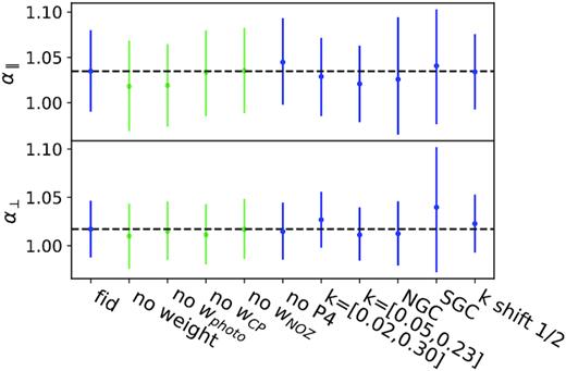
$Best-fitting values of $\alpha_{\parallel}$ and α⊥ for the tests performed on DR16 quasar sample for the BAO-analysis (values are taken from Table 3). Green points show the impact of taking into account the different weights while blue points are for consistency/robustness tests.$

Figure 4.

Best-fitting values of |$\alpha_{\parallel}$| and α_⊥ for the tests performed on DR16 quasar sample for the BAO-analysis (values are taken from Table 3). Green points show the impact of taking into account the different weights while blue points are for consistency/robustness tests.

Table 3.

Best fit and 1-sigma error bars for robustness tests performed on the DR16 data for the BAO-only analysis in Fourier Space. When the shift with respect to the DR16 final result is larger than 0.01, we indicate within parentheses () the standard deviation of the mock-by-mock differences.

	\|$\alpha _{\parallel }$\|	α_⊥	χ²(n_dof)	red.χ²
DR16 final result	1.035 ± 0.045	1.017 ± 0.029	87.63 (126-22)	0.84
No wf	1.033 ± 0.043	1.018 ± 0.028	(126-22)
Coupled	1.016 ± 0.048	1.016 ± 0.031	(126-22)
	(0.029)	(0.017)
No weight	1.018 ± 0.050	1.010 ± 0.034	70.86 (126-22)	0.68
No w_sys	1.019 ± 0.045	1.015 ± 0.030	85.32 (126-22)	0.82
No w_cp	1.034 ± 0.047	1.011 ± 0.031	78.36 (126-22)	0.75
No w_noz	1.035 ± 0.047	1.017 ± 0.031	79.90 (126-22)	0.77
No ℓ = 4	1.045 ± 0.048	1.015 ± 0.030	46.39 (84-16)	0.68
	(0.017)	(0.013)
k = [0.02,0.30]	1.029 ± 0.043	1.027 ± 0.029	107.46 (168-22)	0.74
	(0.017)	(0.014)
k = [0.05,0.23]	1.021 ± 0.042	1.011 ± 0.028	71.57 (108-22)	0.83
	(0.036)	(0.022)
k shift 1/2	1.034 ± 0.042	1.023 ± 0.030	92.41 (126-22)	0.89
\|$\Sigma _\mathrm{ s}=4-2\, {\rm Mpc/h}$\|	1.031 ± 0.042	1.016 ± 0.029	86.06 (126-22)
\|$\Sigma _\mathrm{ s}=4+2\, {\rm Mpc/h}$\|	1.040 ± 0.049	1.017 ± 0.030	89.50(126-22)
NGC	1.026 ± 0.065	1.013 ± 0.033	46.63 (63-12)	0.91
SGC	1.041 ± 0.063	1.040 ± 0.065	41.12 (63-12)	0.81
Isotropic BAO	α_iso = 1.025 ± 0.020		26.76 (42-9)	0.81

	\|$\alpha _{\parallel }$\|	α_⊥	χ²(n_dof)	red.χ²
DR16 final result	1.035 ± 0.045	1.017 ± 0.029	87.63 (126-22)	0.84
No wf	1.033 ± 0.043	1.018 ± 0.028	(126-22)
Coupled	1.016 ± 0.048	1.016 ± 0.031	(126-22)
	(0.029)	(0.017)
No weight	1.018 ± 0.050	1.010 ± 0.034	70.86 (126-22)	0.68
No w_sys	1.019 ± 0.045	1.015 ± 0.030	85.32 (126-22)	0.82
No w_cp	1.034 ± 0.047	1.011 ± 0.031	78.36 (126-22)	0.75
No w_noz	1.035 ± 0.047	1.017 ± 0.031	79.90 (126-22)	0.77
No ℓ = 4	1.045 ± 0.048	1.015 ± 0.030	46.39 (84-16)	0.68
	(0.017)	(0.013)
k = [0.02,0.30]	1.029 ± 0.043	1.027 ± 0.029	107.46 (168-22)	0.74
	(0.017)	(0.014)
k = [0.05,0.23]	1.021 ± 0.042	1.011 ± 0.028	71.57 (108-22)	0.83
	(0.036)	(0.022)
k shift 1/2	1.034 ± 0.042	1.023 ± 0.030	92.41 (126-22)	0.89
\|$\Sigma _\mathrm{ s}=4-2\, {\rm Mpc/h}$\|	1.031 ± 0.042	1.016 ± 0.029	86.06 (126-22)
\|$\Sigma _\mathrm{ s}=4+2\, {\rm Mpc/h}$\|	1.040 ± 0.049	1.017 ± 0.030	89.50(126-22)
NGC	1.026 ± 0.065	1.013 ± 0.033	46.63 (63-12)	0.91
SGC	1.041 ± 0.063	1.040 ± 0.065	41.12 (63-12)	0.81
Isotropic BAO	α_iso = 1.025 ± 0.020		26.76 (42-9)	0.81

Table 3.

Best fit and 1-sigma error bars for robustness tests performed on the DR16 data for the BAO-only analysis in Fourier Space. When the shift with respect to the DR16 final result is larger than 0.01, we indicate within parentheses () the standard deviation of the mock-by-mock differences.

	\|$\alpha _{\parallel }$\|	α_⊥	χ²(n_dof)	red.χ²
DR16 final result	1.035 ± 0.045	1.017 ± 0.029	87.63 (126-22)	0.84
No wf	1.033 ± 0.043	1.018 ± 0.028	(126-22)
Coupled	1.016 ± 0.048	1.016 ± 0.031	(126-22)
	(0.029)	(0.017)
No weight	1.018 ± 0.050	1.010 ± 0.034	70.86 (126-22)	0.68
No w_sys	1.019 ± 0.045	1.015 ± 0.030	85.32 (126-22)	0.82
No w_cp	1.034 ± 0.047	1.011 ± 0.031	78.36 (126-22)	0.75
No w_noz	1.035 ± 0.047	1.017 ± 0.031	79.90 (126-22)	0.77
No ℓ = 4	1.045 ± 0.048	1.015 ± 0.030	46.39 (84-16)	0.68
	(0.017)	(0.013)
k = [0.02,0.30]	1.029 ± 0.043	1.027 ± 0.029	107.46 (168-22)	0.74
	(0.017)	(0.014)
k = [0.05,0.23]	1.021 ± 0.042	1.011 ± 0.028	71.57 (108-22)	0.83
	(0.036)	(0.022)
k shift 1/2	1.034 ± 0.042	1.023 ± 0.030	92.41 (126-22)	0.89
\|$\Sigma _\mathrm{ s}=4-2\, {\rm Mpc/h}$\|	1.031 ± 0.042	1.016 ± 0.029	86.06 (126-22)
\|$\Sigma _\mathrm{ s}=4+2\, {\rm Mpc/h}$\|	1.040 ± 0.049	1.017 ± 0.030	89.50(126-22)
NGC	1.026 ± 0.065	1.013 ± 0.033	46.63 (63-12)	0.91
SGC	1.041 ± 0.063	1.040 ± 0.065	41.12 (63-12)	0.81
Isotropic BAO	α_iso = 1.025 ± 0.020		26.76 (42-9)	0.81

	\|$\alpha _{\parallel }$\|	α_⊥	χ²(n_dof)	red.χ²
DR16 final result	1.035 ± 0.045	1.017 ± 0.029	87.63 (126-22)	0.84
No wf	1.033 ± 0.043	1.018 ± 0.028	(126-22)
Coupled	1.016 ± 0.048	1.016 ± 0.031	(126-22)
	(0.029)	(0.017)
No weight	1.018 ± 0.050	1.010 ± 0.034	70.86 (126-22)	0.68
No w_sys	1.019 ± 0.045	1.015 ± 0.030	85.32 (126-22)	0.82
No w_cp	1.034 ± 0.047	1.011 ± 0.031	78.36 (126-22)	0.75
No w_noz	1.035 ± 0.047	1.017 ± 0.031	79.90 (126-22)	0.77
No ℓ = 4	1.045 ± 0.048	1.015 ± 0.030	46.39 (84-16)	0.68
	(0.017)	(0.013)
k = [0.02,0.30]	1.029 ± 0.043	1.027 ± 0.029	107.46 (168-22)	0.74
	(0.017)	(0.014)
k = [0.05,0.23]	1.021 ± 0.042	1.011 ± 0.028	71.57 (108-22)	0.83
	(0.036)	(0.022)
k shift 1/2	1.034 ± 0.042	1.023 ± 0.030	92.41 (126-22)	0.89
\|$\Sigma _\mathrm{ s}=4-2\, {\rm Mpc/h}$\|	1.031 ± 0.042	1.016 ± 0.029	86.06 (126-22)
\|$\Sigma _\mathrm{ s}=4+2\, {\rm Mpc/h}$\|	1.040 ± 0.049	1.017 ± 0.030	89.50(126-22)
NGC	1.026 ± 0.065	1.013 ± 0.033	46.63 (63-12)	0.91
SGC	1.041 ± 0.063	1.040 ± 0.065	41.12 (63-12)	0.81
Isotropic BAO	α_iso = 1.025 ± 0.020		26.76 (42-9)	0.81

We measure the difference in the best-fitting parameters between the decoupled and the coupled smooth-term prescriptions, and we observe variations of the order of 0.019 for |$\alpha _{\parallel }$| and 0.001 for α_⊥. Using the EZmocks, we found that the standard deviations of the mock-by-mock differences are σ_mocks(⁠|$\alpha _{\parallel }$|⁠) = 0.029 and σ_mocks(⁠|$\alpha _{\parallel }$|⁠) = 0.017. Therefore, the observed variation is within statistics and we do not assign any additional systematic error to cope with this effect.

Then, we show the impact of the different weights on the cosmological parameters estimation. It appears that taking into account photometric weight has the largest impact although the overall effect is smaller than half the statistical precision. The fibre collision and spectroscopic redshift weights have only a marginal effect on the best-fitting parameters. Not taking into account the hexadecapole in the fit changes |$\alpha _{\parallel }$| by 0.010 and α_⊥ by 0.02.

Changing the fitting range for the BAO analysis is also studied. First, the upper bound is increased to |$k=0.3\, \mathrm{h}\cdot \mathrm{Mpc}^{-1}{}$| bringing in scales for which BAO oscillations are no longer visible in the data. Adding these data produces an effect of Δα_⊥ = 0.010, which is the largest deviation in the tests that were done for this parameter. It is due to the fact that the added data put a stronger constraint on the broad-band terms in a region without BAO signal and therefore remove the ability of the model to account for broad-band variations in the region of higher BAO significance. Adding more terms in the broad-band polynomial expansion could relieve this effect but this goes beyond the validation of the model that was performed in the mock challenge. Removing scales below |$k\lt 0.05\, \mathrm{h}\cdot \mathrm{Mpc}^{-1}{}$| has a noticeable effect on the radial dilation scale Δ|$\alpha _{\parallel }$| = 0.014 as it removes scales where the amplitude of the BAO wiggles is large as can be seen for the mocks in Fig. 3. The differences when changing the upper or lower bound of the k-range are within one standard deviation of the differences observed in the EZmocks. Shifting the k-bins by half the bin width (⁠|$\Delta k=0.005\, \mathrm{h}\cdot \mathrm{Mpc}^{-1}{}$|⁠) has a minor impact.

We also study the variation in the best-fitting parameters when changing the strength of the damping terms that are determined using the OuterRim mocks. We observe variations that are at the level of 0.1 per cent for extreme changes of ±30 per cent in |$\Sigma _{\parallel }$| and Σ_⊥. In the case of Σ_s, the sensitivity on |$\alpha _{\parallel }$| is larger, reaching 0.5 per cent for variations of ΔΣ_s = ±50 per cent as shown in the bottom part of Table 3. The observed changes in cosmological parameters are taken as a systematic error due to the knowledge of the damping strength:

$$\begin{eqnarray*} \Delta (\alpha _\parallel)\!\!\left.\right|_\mathrm{damping}=0.005\quad \Delta (\alpha _\perp)\!\!\left.\right|_\mathrm{damping}=0.001. \end{eqnarray*}$$

(28)

Furthermore, the error on |$\alpha _{\parallel }$| is affected by the change in the damping term as our data have a sharp BAO feature and the fit prefers less damping. The statistical errors that we measure using our fiducial choice of damping parameters are close to the average of the errors on |$\alpha _{\parallel }$| and α_⊥ for the various cases that were studied.

The fit was also performed for each galactic cap separately and the differences observed are within the variations expected from the statistics. One should note that, because the strength of the BAO for each cap is different, the precision on the best-fitting parameters does not follow the difference in surface area of each sub-sample (see Table 1).

The systematic errors on |$\alpha _{\parallel }$| and α_⊥ for the BAO analysis are summarized in Table 4. The dominant contribution stems from the error in the modelling. Adding systematic errors contributions in quadrature, we obtain a 1.2 per cent error on |$\alpha _{\parallel }$| and 0.7 per cent on α_⊥. These errors represent approximately 25 per cent of the statistical errors.

Table 4.

Systematic errors on the estimate of the cosmological parameters from the BAO analysis.

	\|$\alpha _{\parallel }$\|	α_⊥
Observational	0.0037	0.0036
Modelling	0.0098	0.0055
Damping	0.005	0.001
Total systematics	0.012	0.007
Statistical error	0.045	0.029
Fraction	27%	24%

	\|$\alpha _{\parallel }$\|	α_⊥
Observational	0.0037	0.0036
Modelling	0.0098	0.0055
Damping	0.005	0.001
Total systematics	0.012	0.007
Statistical error	0.045	0.029
Fraction	27%	24%

Table 4.

Systematic errors on the estimate of the cosmological parameters from the BAO analysis.

	\|$\alpha _{\parallel }$\|	α_⊥
Observational	0.0037	0.0036
Modelling	0.0098	0.0055
Damping	0.005	0.001
Total systematics	0.012	0.007
Statistical error	0.045	0.029
Fraction	27%	24%

	\|$\alpha _{\parallel }$\|	α_⊥
Observational	0.0037	0.0036
Modelling	0.0098	0.0055
Damping	0.005	0.001
Total systematics	0.012	0.007
Statistical error	0.045	0.029
Fraction	27%	24%

3.2.2 Results from the BAO analysis and consensus

The results of our analysis are compared to the BAO analysis performed in configuration space, which is described in our companion paper (Hou et al. 2020). In Fig. 5, we show the variation of the minimum χ² of our model as a function of the assumed isotropic dilation scale α_iso and compare it with the χ² for the model without BAO oscillations. This shows that our data confirm the presence of the BAO signal at the 5- to 6-σ level, in agreement with the results obtained in configuration space (Hou et al. 2020).

Figure 5.

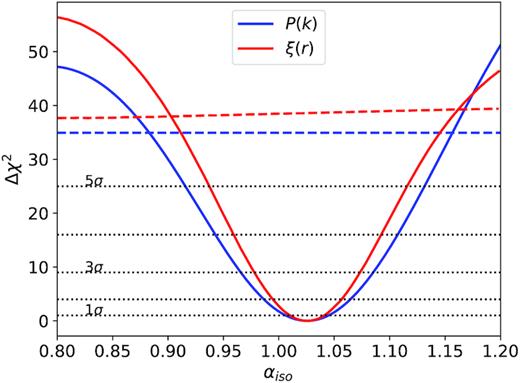
χ² profile of the α_iso BAO parameter in Fourier and configuration space. We show the χ² profile for the BAO model (solid curves) and the χ² difference between a model without BAO peak and the minimum of the BAO model (dashed lines).

In Fig. 6, we compare the parameters measured in configuration and Fourier Space for the 1000 approximate mocks. After selecting mocks for which there is a clear detection of the BAO signal in either analysis (the selection criteria is 0.82 < [|$\alpha _{\parallel }$|⁠, α_⊥] < 1.18 keeping 742/1000 mocks), the Pearson correlation coefficients reach ρ(⁠|$\alpha _{\parallel }$|⁠) = 0.795 and ρ(α_⊥) = 0.821. The errors in |$\alpha _{\parallel }$| and α_⊥ obtained in configuration space are comparable to the errors from the power spectrum fits, although the errors in configuration space, on average, tend be larger in the low S/N regime. The DR16 measurements are shown by the red points in the left-hand panel Fig. 6. The errors measured from the DR16 data are at the edge of the distribution of the EZmocks for both analyses. This is expected since the BAO signal observed in the data is stronger than the average BAO signal in the mocks, as was shown in Fig. 3.

Figure 6.

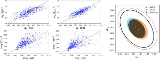
Left: Comparison of the cosmological parameters and errors measured in the BAO analysis of the 2-point correlation function analysis, from Hou et al. (2020) (vertical axis), and of the power spectrum analysis (horizontal axis). The blue points show values of the EZmocks fit while the red point stands for the DR16 measurement. Right: Likelihood contour for the two analyses and the consensus. The orange (blue) contours represent the power spectrum (2-point correlation function) analysis; the black contours represent the consensus.

In the right-hand panel of Fig. 6, we compare the likelihood contours obtained for the Fourier and configuration space BAO analyses as well as the consensus result. The results are in good agreement, as the difference between the two represents only 30 per cent of the standard deviation of the mock-by-mock differences for both |$a _{\parallel }$| and a_⊥.

Then, following Sánchez et al. (2017), we perform a consensus analysis by computing :

$$\begin{eqnarray*} D_\mathrm{ c}=\Psi _\mathrm{ c}^{-1}\sum _{i=1}^m \sum _{j=1}^m\Psi _{\mathrm{ tot},\mathrm{ \mathit{ ji}}}D_i, \end{eqnarray*}$$

(29)

where D_c is the parameter consensus vector, Ψ_c is the inverse of the consensus covariance matrix, m is the number of different statistical analyses (in this case, m = 2), and Ψ_tot is the inverse of the total covariance matrix (each Ψ_tot,_ji term is a p × p matrix with p the number of parameters). The cross-covariance matrix elements are measured using the approximate mocks while the diagonal comes from the covariance matrix of the individual data fits. We convert the dilation scale parameters to the cosmological parameters D_H/r_drag and D_M/r_drag with equation (12). The final results of these cosmological parameters for the BAO analysis in Fourier and configuration spaces and their consensus are given in Table 5. We present the consensus covariance matrix including the statistical errors, the modelling systematics, and the observational systematics:

$$\begin{eqnarray*} {\rm C}_{\rm bao}=\begin{pmatrix}& D_{\rm H}/r_{\rm drag} & D_{\rm M}/r_{\rm drag} \\ & 0.3047 & 0.1707 \\ & - & 0.6373 \\ \end{pmatrix} . \end{eqnarray*}$$

(30)

The consensus results are used to derive the cosmological implications of the eBOSS data (eBOSS Collaboration 2020).

Table 5.

Final results of the BAO-only analyses in Fourier and configuration spaces and their consensus.

	D_H(z_eff)/r_drag	D_M(z_eff)/r_drag	D_V(z_eff)/r_drag
Fourier Space	13.34 ± 0.60	30.60 ± 0.90	26.50 ± 0.55
Configuration space	13.22 ± 0.58	30.82 ± 0.85	26.52 ± 0.44
BAO-only consensus	13.26 ± 0.55	30.69 ± 0.80	26.51 ± 0.42

	D_H(z_eff)/r_drag	D_M(z_eff)/r_drag	D_V(z_eff)/r_drag
Fourier Space	13.34 ± 0.60	30.60 ± 0.90	26.50 ± 0.55
Configuration space	13.22 ± 0.58	30.82 ± 0.85	26.52 ± 0.44
BAO-only consensus	13.26 ± 0.55	30.69 ± 0.80	26.51 ± 0.42

Table 5.

Final results of the BAO-only analyses in Fourier and configuration spaces and their consensus.

	D_H(z_eff)/r_drag	D_M(z_eff)/r_drag	D_V(z_eff)/r_drag
Fourier Space	13.34 ± 0.60	30.60 ± 0.90	26.50 ± 0.55
Configuration space	13.22 ± 0.58	30.82 ± 0.85	26.52 ± 0.44
BAO-only consensus	13.26 ± 0.55	30.69 ± 0.80	26.51 ± 0.42

	D_H(z_eff)/r_drag	D_M(z_eff)/r_drag	D_V(z_eff)/r_drag
Fourier Space	13.34 ± 0.60	30.60 ± 0.90	26.50 ± 0.55
Configuration space	13.22 ± 0.58	30.82 ± 0.85	26.52 ± 0.44
BAO-only consensus	13.26 ± 0.55	30.69 ± 0.80	26.51 ± 0.42

4 FULL-SHAPE RSD ANALYSIS

In this section, we present the Full-Shape RSD analysis of the eBOSS DR16 quasar power spectrum. First, we briefly describe the power spectrum model and then we present the various tests performed both on the EZmocks and on the data to estimate the systematic errors in our measurement. Finally, we present the results we obtain and perform a consensus analysis with the measurement in the configuration space for the same sample as presented in Hou et al. (2020).

4.1 Model

The RSD model used in this analysis is based on the work of Taruya et al. (2010). We use the implementation of de Mattia et al. (2020) and we refer the reader to Section 3.1 of this paper for further details. In this model, the non-linear power spectrum for a tracer of the matter distribution, with bias b₁, is given by:

$$\begin{eqnarray*} P_\mathrm{ q}(k,\mu) &=& P_{\mathrm{ q},\delta \delta }(k)+2f\mu ^2P_{\mathrm{ \mathrm{ q}},\delta \theta }(k)+f^2\mu ^4P_{\mathrm{ q},\theta \theta }(k)\nonumber \\ && + \, b_1^3A(k,\mu ,f/b_1)+b_1^4B(k,\mu ,f/b_1) , \end{eqnarray*}$$

(31)

where P_{q, δδ}, P_{q, δθ}, and P_{q, θθ} are the quasar–quasar, quasar–velocity, and velocity–velocity power spectra, respectively, and A and B are correction terms to account for the non-linearity of the real to redshift space mapping. The 1-loop bias terms are taken from McDonald & Roy (2009) and all terms are calculated at two-loop order following the RegPT scheme (Taruya 2014).It is worth noting that in the bias expansion of P_{q, δδ}, there is an additional term, |$N_\mathrm{ g} = A_\mathrm{ g} P_0^{\rm noise}$|⁠, to account for the constant galaxy stochasticity.

The power spectrum of the quasars, |${\cal P}_\mathrm{ q}(k,\mu)$|⁠, is the product of the non-linear power spectrum P_q(k, μ) (defined in equation 31) for a biased tracer and of a damping term D, which takes into account non-linear effects that are not included in the matter power spectrum,

$$\begin{eqnarray*} {\cal P}_\mathrm{ q}(k,\mu)=P_\mathrm{ q}(k,\mu)D(k,\mu). \end{eqnarray*}$$

(32)

Following Hou et al. (2018), we use a damping term, which comprises a Gaussian and a Lorentzian-like term a_vir ,

$$\begin{eqnarray*} D=\frac{1}{\sqrt{1+(k\mu a_{\rm vir})^2}}\exp {\left[-\frac{(k\mu \sigma _v)^2}{1+(k\mu a_{\rm vir})^2}\right]}, \end{eqnarray*}$$

(33)

where σ_v is the velocity dispersion, and a_vir is associated with the virial motion of quasars in the dark matter halo they inhabit. In the approach adopted here, we consider redshift errors as an additional velocity dispersion, and we let σ_v vary as a free parameter in order to cope for this effect. We do not add an extra term as in Hou et al. (2018).

Furthermore, the window function measured from the data is applied to the model following the same method that was used for the BAO analysis.

For the fiducial analysis, the fit is performed over the range |$k=[0.02, 0.3]\, \mathrm{h}\cdot \mathrm{Mpc}^{-1}$| and 13 parameters are allowed to vary. The cosmological parameters (α_⊥, |$\alpha _{\parallel }$|⁠, f) are common to the two galactic caps, while the parameters of the bias expansion (b₁, b₂), the shot-noise term (A_g) and of the damping term (σ_v, a_vir), are allowed to be different for the two galactic caps. We use flat priors for all parameters, and the intervals of variations are given in Table 6 and are chosen such that the boundaries are not hit.

Table 6.

Interval of variations of the parameters used in the χ² minimization for the Full-Shape RSD analysis.

Parameter	Prior range
b₁	(0, 5)
b₂	(−8, 8)
\|$a _{\parallel }$\|	(0.5, 1.5)
a_⊥	(0.5, 1.5)
f	(0.3, 3)
A_g	(−1, 5)
σ_v	(0, 15)
a_vir	(0, 15)

Table 6.

Interval of variations of the parameters used in the χ² minimization for the Full-Shape RSD analysis.

Parameter	Prior range
b₁	(0, 5)
b₂	(−8, 8)
\|$a _{\parallel }$\|	(0.5, 1.5)
a_⊥	(0.5, 1.5)
f	(0.3, 3)
A_g	(−1, 5)
σ_v	(0, 15)
a_vir	(0, 15)

4.2 Validation of the model

We validate our model using the OuterRim mocks described in Section 2.3.2. This is described in detail in the companion paper of Smith et al. (2020), and we give only the main results here. In a first stage, we used the non-blind mocks, which include various redshift-smearing prescriptions to test the damping term, D, introduced in the previous paragraph. We fit our power spectrum model to the 100 realizations of each HOD model and compute the average of the best-fitting parameters. The results show that the true values of |$\alpha _{\parallel }$| and α_⊥ can be recovered to better than 1 per cent and that fσ₈ can be recovered to better than 3 per cent regardless of the redshift-smearing prescription.

In a second stage, we analysed the ‘blind’ set of mocks, whose cosmology is unknown, using the OuterRim fiducial cosmology. The results of the average fit parameters for the 24 sets of mocks with different HOD and different cosmologies are given in section 6.3 of Smith et al. (2020). From the distribution of the results that we obtain, we determine the rms value to be our systematic error on the modelling:

$$\begin{eqnarray*} \Delta \alpha _\parallel \!\!\left.\right|_\mathrm{model}=0.0098 \quad \Delta \alpha _\perp \!\!\left.\right|_\mathrm{model}=0.0066 \quad \Delta f\sigma _8\!\!\left.\right|_\mathrm{model}=0.0123. \nonumber \\ \end{eqnarray*}$$

(34)

4.3 Results

We perform the Full-Shape RSD analysis of the monopole, quadrupole, and hexadecapole of the power spectrum measured from the QSO DR16 catalogue, as described in Section 4.1. The covariance matrix is computed from the 1000 EZmocks. Fig. 7 shows the best-fitting model (solid lines) to the data (points) with NGC and SGC fitted simultaneously. We take the mean of the samples of the Markov chains as final results for the Full-Shape RSD analysis in Fourier Space:

$$\begin{eqnarray*} \alpha _\parallel =1.049 \pm 0.038 \, \alpha _\perp =1.020 \pm 0.029 \, f\sigma _8=0.476 \pm 0.044, \nonumber \\ \end{eqnarray*}$$

(35)

where the errors are computed from the standard deviation of the samples of the chains. In this section, we discuss the evaluation of the systematic errors entering our measurement. We use the EZmocks to quantify the impact of the different weights (fibre collisions, photometric conditions, redshift efficiency). Fibre collisions weights have a large impact and require an improvement of the power spectrum model that is presented. Taking into account the RIC induced by the generation of the random catalogue is also evaluated. At the end of the section, we present the results of robustness tests performed on the DR16 data and show the impact of the different analysis choices on the final results. For the estimation of the systematic errors using the 1000 approximate mocks, we measure the distributions of the mock-by-mock differences. These distributions are fit with a Gaussian from which the mean values and their errors are determined assuming the differences distributions follow Poisson statistics. We take the largest quantity between the mean value or twice the error as a systematic error.

Figure 7.

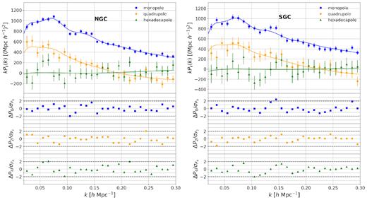
Power spectrum multipoles of the NGC (left) and SGC (right) quasar samples (top panel) and residuals (lower panels) from the NGC and SGC combined fit for the Full-Shape RSD analysis. The points are the data, and the solid lines show the best-fitting model.

4.3.1 Systematic checks

In Fig. 8, we show the change in the power spectrum multipoles when different combinations of systematic effects are included. In each case, the effects are applied to the EZmock catalogues and are corrected for according to the weighting scheme used on the data. It appears that largest systematic offset arises from fibre collisions, and no difference between the two galactic caps is observed beyond the expected statistical error. The impact of the systematic effects on the best-fitting parameters is shown in Table 7 for the average of the 1000 EZmocks and for the combined NGC + SGC fit. In this table, the lines that start with a Δ show the difference in offset between the preceding line with respect to the offset measured for the line described within parentheses. It shows that not correcting for fibre collisions leads to large systematic offsets on all cosmological parameters that go up to 5 per cent for the case of the fσ₈.

Figure 8.

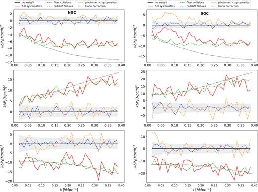
Shifts on the power spectrum multipoles induced by the systematic effects applied to the EZ mocks on the NGC (left-hand panels) and SGC (right-hand panels). The dashed line represents the effect of fibre collisions weights (green) of photometric systematic weights (yellow) and redshift failures weights (blue). The effect of all weights together is shown as the red solid line. The black dotted lines show the full correction for fibre collision as proposed by Hahn et al. (2017). The grey-shaded region represents the statistical error.

Table 7.

Average value of the cosmological parameters recovered from the fits of 1000 EZmocks under different systematic effects applied to the catalogues and corrected for using the standard weighting scheme. The lines that start with a Δ show the difference in offset between the preceding line with respect to the offset measured for the line described within parentheses. The ‘expected’ values for the dilation scales are not unity since the EZmocks cosmology is slightly different from the fiducial cosmology.

Tests on mocks	\|$\alpha _{\parallel }$\|	α_⊥	fσ₈
Expected	1.004	1.002	0.379
Ref : no weights	0.988 ± 0.002	0.990 ± 0.001	0.380 ± 0.002
w_nozw_sys	0.988 ± 0.002	0.992 ± 0.001	0.382 ± 0.002
Δ₁ wrt (ref)	−0.0006(15)	0.0019(12)	0.0026(14)
w_q = w_nozw_sysw_cp	0.974 ± 0.002	0.999 ± 0.001	0.399 ± 0.002
\|$\, \Delta$\| wrt (w_nozw_sys)	−0.0147(9)	0.0081(7)	0.0166(9)
\|$w_\mathrm{ q}+\Delta P_{\mathrm{ cp}}^{u}$\|	0.991 ± 0.002	0.989 ± 0.001	0.380 ± 0.002
\|$\, \Delta _2$\| wrt (w_q)	0.0172(6)	−0.0107(6)	−0.0205(6)
\|$w_\mathrm{ q}+\Delta P_{\rm cp}^{u}+\Delta P_{\rm cp}^{c}$\|	0.991 ± 0.002	0.990 ± 0.001	0.381 ± 0.002
\|$\, \Delta$\| wrt (⁠\|$w_\mathrm{ q}+\Delta P_{\rm cp}^{u}$\|⁠)	0.0008(6)	0.0007(5)	0.0024(6)
\|$\, \Delta _3$\| wrt (w_nozw_sys)	0.0040(9)	−0.0018(7)	−0.0011(10)
\|$\, \Delta$\| wrt (ref)	0.0056(15)	−0.0000(13)	0.0007(15)
No RIC	0.995 ± 0.002	0.986 ± 0.001	0.381 ± 0.002
\|$\, \Delta _4$\| wrt (ref)	0.0074(8)	−0.0039(6)	0.0004(8)
RIC corrected	1.001 ± 0.002	0.985 ± 0.001	0.383 ± 0.002
\|$\, \Delta _5$\| wrt (⁠\|$w_\mathrm{ q}+\Delta P_{\rm cp}^{u}$\|⁠)	0.0077(1)	−0.0047(1)	0.0015(1)

Tests on mocks	\|$\alpha _{\parallel }$\|	α_⊥	fσ₈
Expected	1.004	1.002	0.379
Ref : no weights	0.988 ± 0.002	0.990 ± 0.001	0.380 ± 0.002
w_nozw_sys	0.988 ± 0.002	0.992 ± 0.001	0.382 ± 0.002
Δ₁ wrt (ref)	−0.0006(15)	0.0019(12)	0.0026(14)
w_q = w_nozw_sysw_cp	0.974 ± 0.002	0.999 ± 0.001	0.399 ± 0.002
\|$\, \Delta$\| wrt (w_nozw_sys)	−0.0147(9)	0.0081(7)	0.0166(9)
\|$w_\mathrm{ q}+\Delta P_{\mathrm{ cp}}^{u}$\|	0.991 ± 0.002	0.989 ± 0.001	0.380 ± 0.002
\|$\, \Delta _2$\| wrt (w_q)	0.0172(6)	−0.0107(6)	−0.0205(6)
\|$w_\mathrm{ q}+\Delta P_{\rm cp}^{u}+\Delta P_{\rm cp}^{c}$\|	0.991 ± 0.002	0.990 ± 0.001	0.381 ± 0.002
\|$\, \Delta$\| wrt (⁠\|$w_\mathrm{ q}+\Delta P_{\rm cp}^{u}$\|⁠)	0.0008(6)	0.0007(5)	0.0024(6)
\|$\, \Delta _3$\| wrt (w_nozw_sys)	0.0040(9)	−0.0018(7)	−0.0011(10)
\|$\, \Delta$\| wrt (ref)	0.0056(15)	−0.0000(13)	0.0007(15)
No RIC	0.995 ± 0.002	0.986 ± 0.001	0.381 ± 0.002
\|$\, \Delta _4$\| wrt (ref)	0.0074(8)	−0.0039(6)	0.0004(8)
RIC corrected	1.001 ± 0.002	0.985 ± 0.001	0.383 ± 0.002
\|$\, \Delta _5$\| wrt (⁠\|$w_\mathrm{ q}+\Delta P_{\rm cp}^{u}$\|⁠)	0.0077(1)	−0.0047(1)	0.0015(1)

Table 7.

Average value of the cosmological parameters recovered from the fits of 1000 EZmocks under different systematic effects applied to the catalogues and corrected for using the standard weighting scheme. The lines that start with a Δ show the difference in offset between the preceding line with respect to the offset measured for the line described within parentheses. The ‘expected’ values for the dilation scales are not unity since the EZmocks cosmology is slightly different from the fiducial cosmology.

Tests on mocks	\|$\alpha _{\parallel }$\|	α_⊥	fσ₈
Expected	1.004	1.002	0.379
Ref : no weights	0.988 ± 0.002	0.990 ± 0.001	0.380 ± 0.002
w_nozw_sys	0.988 ± 0.002	0.992 ± 0.001	0.382 ± 0.002
Δ₁ wrt (ref)	−0.0006(15)	0.0019(12)	0.0026(14)
w_q = w_nozw_sysw_cp	0.974 ± 0.002	0.999 ± 0.001	0.399 ± 0.002
\|$\, \Delta$\| wrt (w_nozw_sys)	−0.0147(9)	0.0081(7)	0.0166(9)
\|$w_\mathrm{ q}+\Delta P_{\mathrm{ cp}}^{u}$\|	0.991 ± 0.002	0.989 ± 0.001	0.380 ± 0.002
\|$\, \Delta _2$\| wrt (w_q)	0.0172(6)	−0.0107(6)	−0.0205(6)
\|$w_\mathrm{ q}+\Delta P_{\rm cp}^{u}+\Delta P_{\rm cp}^{c}$\|	0.991 ± 0.002	0.990 ± 0.001	0.381 ± 0.002
\|$\, \Delta$\| wrt (⁠\|$w_\mathrm{ q}+\Delta P_{\rm cp}^{u}$\|⁠)	0.0008(6)	0.0007(5)	0.0024(6)
\|$\, \Delta _3$\| wrt (w_nozw_sys)	0.0040(9)	−0.0018(7)	−0.0011(10)
\|$\, \Delta$\| wrt (ref)	0.0056(15)	−0.0000(13)	0.0007(15)
No RIC	0.995 ± 0.002	0.986 ± 0.001	0.381 ± 0.002
\|$\, \Delta _4$\| wrt (ref)	0.0074(8)	−0.0039(6)	0.0004(8)
RIC corrected	1.001 ± 0.002	0.985 ± 0.001	0.383 ± 0.002
\|$\, \Delta _5$\| wrt (⁠\|$w_\mathrm{ q}+\Delta P_{\rm cp}^{u}$\|⁠)	0.0077(1)	−0.0047(1)	0.0015(1)

Tests on mocks	\|$\alpha _{\parallel }$\|	α_⊥	fσ₈
Expected	1.004	1.002	0.379
Ref : no weights	0.988 ± 0.002	0.990 ± 0.001	0.380 ± 0.002
w_nozw_sys	0.988 ± 0.002	0.992 ± 0.001	0.382 ± 0.002
Δ₁ wrt (ref)	−0.0006(15)	0.0019(12)	0.0026(14)
w_q = w_nozw_sysw_cp	0.974 ± 0.002	0.999 ± 0.001	0.399 ± 0.002
\|$\, \Delta$\| wrt (w_nozw_sys)	−0.0147(9)	0.0081(7)	0.0166(9)
\|$w_\mathrm{ q}+\Delta P_{\mathrm{ cp}}^{u}$\|	0.991 ± 0.002	0.989 ± 0.001	0.380 ± 0.002
\|$\, \Delta _2$\| wrt (w_q)	0.0172(6)	−0.0107(6)	−0.0205(6)
\|$w_\mathrm{ q}+\Delta P_{\rm cp}^{u}+\Delta P_{\rm cp}^{c}$\|	0.991 ± 0.002	0.990 ± 0.001	0.381 ± 0.002
\|$\, \Delta$\| wrt (⁠\|$w_\mathrm{ q}+\Delta P_{\rm cp}^{u}$\|⁠)	0.0008(6)	0.0007(5)	0.0024(6)
\|$\, \Delta _3$\| wrt (w_nozw_sys)	0.0040(9)	−0.0018(7)	−0.0011(10)
\|$\, \Delta$\| wrt (ref)	0.0056(15)	−0.0000(13)	0.0007(15)
No RIC	0.995 ± 0.002	0.986 ± 0.001	0.381 ± 0.002
\|$\, \Delta _4$\| wrt (ref)	0.0074(8)	−0.0039(6)	0.0004(8)
RIC corrected	1.001 ± 0.002	0.985 ± 0.001	0.383 ± 0.002
\|$\, \Delta _5$\| wrt (⁠\|$w_\mathrm{ q}+\Delta P_{\rm cp}^{u}$\|⁠)	0.0077(1)	−0.0047(1)	0.0015(1)

There is an effect of imperfectly correcting for photometric conditions, which affects the monopole (yellow dashed curves in Fig. 8). The shift is located at small k and amounts to about 1|${{\ \rm per\ cent}}$| of the observed monopole and no effect beyond statistics is observed in the higher order multipoles. The shift is higher in the SGC for which the spread of the photometric weights is known to be larger than the NGC (see fig. 12 of Zarrouk et al. 2018). The best-fitting parameters are slightly modified by the amount given in the line Δ₁ of Table 7 that shows the impact of photometric weights and redshift failures together. This difference is then taken as an estimate of the systematic errors arising from photometric conditions.

Taking into account, fibre collision has received much attention, and solutions have been proposed to mitigate their effect on the power spectrum (Hand et al. 2017) and on the 2-point correlation function (Percival & Bianchi 2017). In the approximate method proposed by Hahn et al. (2017) that we use in this paper, the fact that two targets are colliding is modelled by an additional top-hat window function whose width is given by the collision radius D_fc at the effective redshift (⁠|$D_{\rm fc}(z=1.480)=0.9\, \mathrm{h}^{-1}\mathrm{Mpc}$|⁠). In the case the fibre collided objects are uncorrelated, the corrected power spectrum is given by:

$$\begin{eqnarray*} \Delta P_\ell ^{\rm uncorr}(k)=-f_\mathrm{ s} (2l+1)L_\ell (0) \frac{(\pi D_{\rm fc})^2}{k} W_{2\mathrm{ D}}(kD_{\rm fc}), \end{eqnarray*}$$

(36)

where W_x = 2J₁(x)/x is the cylindrical top-hat function in 2D (J₁ is the first kind and first-order Bessel function), and f_s is the fraction of the survey affected by fibre collisions. The latter is determined from the data targets and observational catalogues. Its estimation requires running the tiling algorithm on the full target set, which includes ‘legacy’ objects that have been observed prior to eBOSS, and comparing this to the number of collisions that were actually corrected for in our sample. Our estimation leads to

$$\begin{eqnarray*} f_\mathrm{ s}(\mathrm{ NGC})=0.36 \quad f_\mathrm{ s}(\mathrm{ SGC})=0.45. \end{eqnarray*}$$

(37)

It is substantially lower than the fraction of area of the survey where plates are non-overlapping and collisions are never resolved (60 per cent). It originates from the fact that the ‘legacy’ objects were themselves the result of a tiling algorithm, where collisions were partially resolved. This estimate of f_s was later confirmed to a precision of 10 per cent from the data by measuring the projected correlation function at small transverse scales (see fig. 16 of Hou et al. 2020).

Using the EZmocks, we estimate that for the target density of our sample, |$95{{\ \rm per\ cent}}$| of collisions are uncorrelated. Given that the small-scale clustering of the EZmocks is imperfect, we have confirmed this estimate with the data as it constitutes the dominant part of the correction applied. Nevertheless, as proposed by Hahn et al. (2017), we apply the correction for collisions in the case of correlated objects as:

$$\begin{eqnarray*} \Delta P_\ell ^{\rm corr}(k)=-f_\mathrm{ s} \pi D_{\rm fc}^2 \int \frac{d^2q_{\perp }}{(2 \pi)^2} P(k_{\parallel },q_{\perp })W_{2\mathrm{ D}}(q_{\perp }D_{\rm fc}). \end{eqnarray*}$$

(38)

This correction further decreases the residual offset seen in fσ₈ and does not modify the offset on |$a _{\parallel }$| and a_⊥ (Table 7). The remaining offset after both corrections are applied (line Δ₃ of Table 7) is taken as the systematic error due to fibre collisions. In a companion paper, Mohammad et al. (2020) explore the possibility to use the pair-weighting technique (Percival & Bianchi 2017) for our sample. This method was not used in the present work but its potential for future surveys is indubitable.

The size of the correction given in equation (38) is shown as a dotted line in Fig. 8 that is qualitatively in agreement with the observed systematic shift for all multipoles and also captures the difference between the NGC and the SGC. The agreement is a little worse for the monopole, but this is negligible, since the shift in the monopole is very small compared to its amplitude. After applying this correction to the power spectrum model, the systematic offsets in the best-fitting parameters measured from the EZmocks are reduced by a factor of 5 (Table 7) to an acceptable level of the order of one-tenth of the statistical error on each parameter. The correction depends linearly on the value of f_s that is known to a precision of |$10{{\ \rm per\ cent}}$|⁠. Therefore, we take 10 per cent of the shifts due to this effect (line Δ₂ of Table 7) as a systematic error.

It has been recently shown by de Mattia & Ruhlmann-Kleider (2019) that drawing the redshifts of the random catalogues from the data catalogue introduces a radial integral constraint (RIC). We measure the impact of the RIC on the EZmocks by producing a large random catalogue that samples the random catalogues of all the mocks. The observed shift, given in line Δ₄ of Table 7, shows that correction that would need to be applied to correct for the RIC is of the order of 0.7 per cent on |$\alpha _{\parallel }$|⁠, 0.4 per cent on α_⊥, and no effect is seen on fσ₈. The RIC can be accounted for in the power spectrum model and its effect on cosmological parameter is given in line Δ₅ of Table 7. The agreement with the estimate using different random files is at the per-mil level and we choose, for what follows, to account for the RIC in the model and do not quote systematic errors for this correction.

The observational systematic errors are summarized in Table 8 and summing them in quadrature leads to the following total observational systematic errors:

$$\begin{eqnarray*} \Delta \alpha _\parallel \!\!\left.\right|_\mathrm{obs}=0.005 \quad \Delta \alpha _\perp \!\!\left.\right|_\mathrm{obs}=0.003 \quad \Delta f\sigma _8\!\!\left.\right|_\mathrm{obs}=0.004 . \end{eqnarray*}$$

(39)

Adding the modelling error in quadrature (see Table 8), the total systematic errors on the cosmological parameters from the Full-Shape RSD Fourier Space analysis are:

$$\begin{eqnarray*} \Delta \alpha _\parallel \!\!\left.\right|_\mathrm{syst}=0.011 \quad \Delta \alpha _\perp \!\!\left.\right|_\mathrm{syst}=0.007 \quad \Delta f\sigma _8\!\!\left.\right|_\mathrm{syst}=0.012 . \end{eqnarray*}$$

(40)

These systematic errors represent 30 per cent of the statistical error and the dominant contribution stems from the modelling of the power spectrum.

Table 8.

Systematic errors on the estimate of the cosmological parameters from the Full-Shape RSD analysis. The total observational systematic error is the quadratic sum of the errors given in the first rows of the table. Combining in quadrature with the modelling errors determined from the mock challenge gives the total systematic error.

	\|$\alpha _{\parallel }$\|	α_⊥	fσ₈
Photometry(Δ₁)	±0.0030	±0.0024	±0.0028
\|$\Delta (f_\mathrm{ s})=10\%(\Delta _2$\|⁠)	±0.0017	±0.0011	±0.0021
Fibre collisions (Δ₃)	+0.0040	−0.0018	±0.0020
Total observational	0.0053	0.0032	0.0040
Redshift smearing	0.0036	0.0042	0.0081
Blind challenge	0.0091	0.0051	0.0093
Total modelling	0.0098	0.0066	0.0123
Total systematics	0.0111	0.0073	0.0129
Statistical error	0.0378	0.0289	0.0447
Fraction	30%	25%	29%

	\|$\alpha _{\parallel }$\|	α_⊥	fσ₈
Photometry(Δ₁)	±0.0030	±0.0024	±0.0028
\|$\Delta (f_\mathrm{ s})=10\%(\Delta _2$\|⁠)	±0.0017	±0.0011	±0.0021
Fibre collisions (Δ₃)	+0.0040	−0.0018	±0.0020
Total observational	0.0053	0.0032	0.0040
Redshift smearing	0.0036	0.0042	0.0081
Blind challenge	0.0091	0.0051	0.0093
Total modelling	0.0098	0.0066	0.0123
Total systematics	0.0111	0.0073	0.0129
Statistical error	0.0378	0.0289	0.0447
Fraction	30%	25%	29%

Table 8.

Systematic errors on the estimate of the cosmological parameters from the Full-Shape RSD analysis. The total observational systematic error is the quadratic sum of the errors given in the first rows of the table. Combining in quadrature with the modelling errors determined from the mock challenge gives the total systematic error.

	\|$\alpha _{\parallel }$\|	α_⊥	fσ₈
Photometry(Δ₁)	±0.0030	±0.0024	±0.0028
\|$\Delta (f_\mathrm{ s})=10\%(\Delta _2$\|⁠)	±0.0017	±0.0011	±0.0021
Fibre collisions (Δ₃)	+0.0040	−0.0018	±0.0020
Total observational	0.0053	0.0032	0.0040
Redshift smearing	0.0036	0.0042	0.0081
Blind challenge	0.0091	0.0051	0.0093
Total modelling	0.0098	0.0066	0.0123
Total systematics	0.0111	0.0073	0.0129
Statistical error	0.0378	0.0289	0.0447
Fraction	30%	25%	29%

	\|$\alpha _{\parallel }$\|	α_⊥	fσ₈
Photometry(Δ₁)	±0.0030	±0.0024	±0.0028
\|$\Delta (f_\mathrm{ s})=10\%(\Delta _2$\|⁠)	±0.0017	±0.0011	±0.0021
Fibre collisions (Δ₃)	+0.0040	−0.0018	±0.0020
Total observational	0.0053	0.0032	0.0040
Redshift smearing	0.0036	0.0042	0.0081
Blind challenge	0.0091	0.0051	0.0093
Total modelling	0.0098	0.0066	0.0123
Total systematics	0.0111	0.0073	0.0129
Statistical error	0.0378	0.0289	0.0447
Fraction	30%	25%	29%

In Fig. 9, we show the fit parameters and their errors as measured for the 1000 approximate EZmocks, compared to the DR16 result. Similarly to what was observed for the BAO analysis, the precision of the DR16 sample for the Full-Shape analysis is untypical of the EZmocks and is among the 1 per cent of mocks with the smallest errors. The interpretation of this is that it comes from the fact that the strength of the BAO is weaker in the EZmocks than in the data. We recall here that the agreement between the EZmocks and the DR16 data for the power spectrum is at the level of a few per cent. Therefore, the covariance matrix that is used in the fit is correct to this precision. Furthermore, since the amplitude of the BAO is smaller in the EZmocks than in the data, the systematic effects that were estimated using the EZmocks have a larger dispersion and lead to a conservative estimate of the systematic errors.

Figure 9.

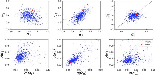
Comparison of the fit parameters and of their errors as measured for the 1000 approximate EZmocks (blue points). The parameters and errors measured for the DR16 sample are represented by a red cross.

4.3.2 Tests on the DR16 sample

We also perform tests to quantify the impact of our choices and for robustness tests to the DR16 data catalogue. Results are summarized in Table 9 and displayed in Fig. 10. First, we quantify the effect of each weight that is used to mitigate systematic effects (see previous section). Then, we vary the fitting conditions to evaluate the impact of the analysis choices that were made on the final results. When the change in cosmological parameters is significant, we compare it with the rms of the mock-by-mock differences distributions and demonstrate that no systematic effect is observed beyond statistics.

Figure 10.

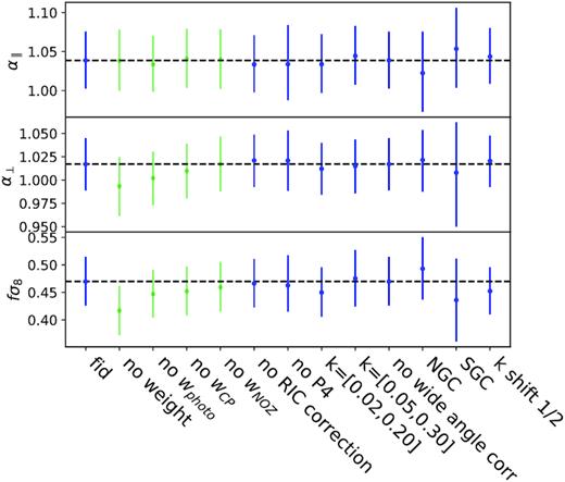
Cosmological parameters measured using the DR16 sample under different choices in the FS analysis. Values of the parameters are taken from Table 9. The subset of green points shows the impact of taking into account different combination of weights to illustrate the size of the correction implied by the weighting scheme but should not be taken as a systematic error.

Table 9.

Best fit and χ² for robustness tests on the data for the Full-Shape RSD analysis. When the difference w.r.t. the reference is significant, we indicate within parentheses () the rms of the mock-by-mock differences observed in the EZmocks under the same conditions.

	\|$\alpha _{\parallel }$\|	α_⊥	fσ₈	b_{1, NGC}σ₈	b_{1, SGC}σ₈	χ²(n_dof)	red.χ²
DR16 best fit	1.039 ± 0.033	1.017 ± 0.025	0.470 ± 0.042	0.960 ± 0.041	0.939 ± 0.040	116.45 (168-13)	0.75
No weight	1.038 ± 0.041	0.993 ± 0.033	0.417 ± 0.046	0.931 ± 0.040	0.916 ± 0.038	95.91 (168-13)	0.62
No w_sys	1.034 ± 0.034	1.002 ± 0.031	0.447 ± 0.044	0.960 ± 0.036	0.946 ± 0.034	115.38 (168-13)	0.74
No w_cp	1.041 ± 0.033	1.010 ± 0.033	0.452 ± 0.045	0.949 ± 0.038	0.930 ± 0.044	104.61 (168-13)	0.67
No w_noz	1.040 ± 0.045	1.017 ± 0.021	0.459 ± 0.043	0.944 ± 0.046	0.916 ± 0.046	106.53 (168-13)	0.69
No RIC correction	1.034 ± 0.035	1.021 ± 0.027	0.466 ± 0.043	0.961 ± 0.041	0.938 ± 0.042	117.00 (168-13)	0.75
No ℓ = 4	1.034 ± 0.056	1.021 ± 0.038	0.463 ± 0.055	0.965 ± 0.035	0.942 ± 0.043	70.51 (112-13)	0.71
	(0.052)	(0.048)	(0.039)
k = (0.02,0.20)	1.034 ± 0.043	1.012 ± 0.024	0.450 ± 0.043	0.968 ± 0.040	0.946 ± 0.046	82.74 (108-13)	0.87
	(0.017)	(0.013)	(0.032)
k = (0.05,0.30)	1.044 ± 0.060	1.015 ± 0.030	0.475 ± 0.058	0.969 ± 0.044	0.931 ± 0.059	104.57 (150-13)	0.76
	(0.018)	(0.015)	(0.020)
k shift 1/2	1.044 ± 0.040	1.020 ± 0.028	0.452 ± 0.045	0.975 ± 0.052	0.954 ± 0.037	125.21 (168-13)	0.81
	(0.019)	(0.017)	(0.019)
No wide angle corr	1.039 ± 0.033	1.017 ± 0.025	0.470 ± 0.042	0.960 ± 0.041	0.939 ± 0.040	116.45 (168-13)	0.75
NGC	1.022 ± 0.047	1.022 ± 0.037	0.493 ± 0.062	0.942 ± 0.054	−	63.91 (84-8)	0.84
SGC	1.054 ± 0.040	1.008 ± 0.041	0.436 ± 0.064	−	0.952 ± 0.044	52.05 (84-8)	0.68

	\|$\alpha _{\parallel }$\|	α_⊥	fσ₈	b_{1, NGC}σ₈	b_{1, SGC}σ₈	χ²(n_dof)	red.χ²
DR16 best fit	1.039 ± 0.033	1.017 ± 0.025	0.470 ± 0.042	0.960 ± 0.041	0.939 ± 0.040	116.45 (168-13)	0.75
No weight	1.038 ± 0.041	0.993 ± 0.033	0.417 ± 0.046	0.931 ± 0.040	0.916 ± 0.038	95.91 (168-13)	0.62
No w_sys	1.034 ± 0.034	1.002 ± 0.031	0.447 ± 0.044	0.960 ± 0.036	0.946 ± 0.034	115.38 (168-13)	0.74
No w_cp	1.041 ± 0.033	1.010 ± 0.033	0.452 ± 0.045	0.949 ± 0.038	0.930 ± 0.044	104.61 (168-13)	0.67
No w_noz	1.040 ± 0.045	1.017 ± 0.021	0.459 ± 0.043	0.944 ± 0.046	0.916 ± 0.046	106.53 (168-13)	0.69
No RIC correction	1.034 ± 0.035	1.021 ± 0.027	0.466 ± 0.043	0.961 ± 0.041	0.938 ± 0.042	117.00 (168-13)	0.75
No ℓ = 4	1.034 ± 0.056	1.021 ± 0.038	0.463 ± 0.055	0.965 ± 0.035	0.942 ± 0.043	70.51 (112-13)	0.71
	(0.052)	(0.048)	(0.039)
k = (0.02,0.20)	1.034 ± 0.043	1.012 ± 0.024	0.450 ± 0.043	0.968 ± 0.040	0.946 ± 0.046	82.74 (108-13)	0.87
	(0.017)	(0.013)	(0.032)
k = (0.05,0.30)	1.044 ± 0.060	1.015 ± 0.030	0.475 ± 0.058	0.969 ± 0.044	0.931 ± 0.059	104.57 (150-13)	0.76
	(0.018)	(0.015)	(0.020)
k shift 1/2	1.044 ± 0.040	1.020 ± 0.028	0.452 ± 0.045	0.975 ± 0.052	0.954 ± 0.037	125.21 (168-13)	0.81
	(0.019)	(0.017)	(0.019)
No wide angle corr	1.039 ± 0.033	1.017 ± 0.025	0.470 ± 0.042	0.960 ± 0.041	0.939 ± 0.040	116.45 (168-13)	0.75
NGC	1.022 ± 0.047	1.022 ± 0.037	0.493 ± 0.062	0.942 ± 0.054	−	63.91 (84-8)	0.84
SGC	1.054 ± 0.040	1.008 ± 0.041	0.436 ± 0.064	−	0.952 ± 0.044	52.05 (84-8)	0.68

Table 9.

Best fit and χ² for robustness tests on the data for the Full-Shape RSD analysis. When the difference w.r.t. the reference is significant, we indicate within parentheses () the rms of the mock-by-mock differences observed in the EZmocks under the same conditions.

	\|$\alpha _{\parallel }$\|	α_⊥	fσ₈	b_{1, NGC}σ₈	b_{1, SGC}σ₈	χ²(n_dof)	red.χ²
DR16 best fit	1.039 ± 0.033	1.017 ± 0.025	0.470 ± 0.042	0.960 ± 0.041	0.939 ± 0.040	116.45 (168-13)	0.75
No weight	1.038 ± 0.041	0.993 ± 0.033	0.417 ± 0.046	0.931 ± 0.040	0.916 ± 0.038	95.91 (168-13)	0.62
No w_sys	1.034 ± 0.034	1.002 ± 0.031	0.447 ± 0.044	0.960 ± 0.036	0.946 ± 0.034	115.38 (168-13)	0.74
No w_cp	1.041 ± 0.033	1.010 ± 0.033	0.452 ± 0.045	0.949 ± 0.038	0.930 ± 0.044	104.61 (168-13)	0.67
No w_noz	1.040 ± 0.045	1.017 ± 0.021	0.459 ± 0.043	0.944 ± 0.046	0.916 ± 0.046	106.53 (168-13)	0.69
No RIC correction	1.034 ± 0.035	1.021 ± 0.027	0.466 ± 0.043	0.961 ± 0.041	0.938 ± 0.042	117.00 (168-13)	0.75
No ℓ = 4	1.034 ± 0.056	1.021 ± 0.038	0.463 ± 0.055	0.965 ± 0.035	0.942 ± 0.043	70.51 (112-13)	0.71
	(0.052)	(0.048)	(0.039)
k = (0.02,0.20)	1.034 ± 0.043	1.012 ± 0.024	0.450 ± 0.043	0.968 ± 0.040	0.946 ± 0.046	82.74 (108-13)	0.87
	(0.017)	(0.013)	(0.032)
k = (0.05,0.30)	1.044 ± 0.060	1.015 ± 0.030	0.475 ± 0.058	0.969 ± 0.044	0.931 ± 0.059	104.57 (150-13)	0.76
	(0.018)	(0.015)	(0.020)
k shift 1/2	1.044 ± 0.040	1.020 ± 0.028	0.452 ± 0.045	0.975 ± 0.052	0.954 ± 0.037	125.21 (168-13)	0.81
	(0.019)	(0.017)	(0.019)
No wide angle corr	1.039 ± 0.033	1.017 ± 0.025	0.470 ± 0.042	0.960 ± 0.041	0.939 ± 0.040	116.45 (168-13)	0.75
NGC	1.022 ± 0.047	1.022 ± 0.037	0.493 ± 0.062	0.942 ± 0.054	−	63.91 (84-8)	0.84
SGC	1.054 ± 0.040	1.008 ± 0.041	0.436 ± 0.064	−	0.952 ± 0.044	52.05 (84-8)	0.68

	\|$\alpha _{\parallel }$\|	α_⊥	fσ₈	b_{1, NGC}σ₈	b_{1, SGC}σ₈	χ²(n_dof)	red.χ²
DR16 best fit	1.039 ± 0.033	1.017 ± 0.025	0.470 ± 0.042	0.960 ± 0.041	0.939 ± 0.040	116.45 (168-13)	0.75
No weight	1.038 ± 0.041	0.993 ± 0.033	0.417 ± 0.046	0.931 ± 0.040	0.916 ± 0.038	95.91 (168-13)	0.62
No w_sys	1.034 ± 0.034	1.002 ± 0.031	0.447 ± 0.044	0.960 ± 0.036	0.946 ± 0.034	115.38 (168-13)	0.74
No w_cp	1.041 ± 0.033	1.010 ± 0.033	0.452 ± 0.045	0.949 ± 0.038	0.930 ± 0.044	104.61 (168-13)	0.67
No w_noz	1.040 ± 0.045	1.017 ± 0.021	0.459 ± 0.043	0.944 ± 0.046	0.916 ± 0.046	106.53 (168-13)	0.69
No RIC correction	1.034 ± 0.035	1.021 ± 0.027	0.466 ± 0.043	0.961 ± 0.041	0.938 ± 0.042	117.00 (168-13)	0.75
No ℓ = 4	1.034 ± 0.056	1.021 ± 0.038	0.463 ± 0.055	0.965 ± 0.035	0.942 ± 0.043	70.51 (112-13)	0.71
	(0.052)	(0.048)	(0.039)
k = (0.02,0.20)	1.034 ± 0.043	1.012 ± 0.024	0.450 ± 0.043	0.968 ± 0.040	0.946 ± 0.046	82.74 (108-13)	0.87
	(0.017)	(0.013)	(0.032)
k = (0.05,0.30)	1.044 ± 0.060	1.015 ± 0.030	0.475 ± 0.058	0.969 ± 0.044	0.931 ± 0.059	104.57 (150-13)	0.76
	(0.018)	(0.015)	(0.020)
k shift 1/2	1.044 ± 0.040	1.020 ± 0.028	0.452 ± 0.045	0.975 ± 0.052	0.954 ± 0.037	125.21 (168-13)	0.81
	(0.019)	(0.017)	(0.019)
No wide angle corr	1.039 ± 0.033	1.017 ± 0.025	0.470 ± 0.042	0.960 ± 0.041	0.939 ± 0.040	116.45 (168-13)	0.75
NGC	1.022 ± 0.047	1.022 ± 0.037	0.493 ± 0.062	0.942 ± 0.054	−	63.91 (84-8)	0.84
SGC	1.054 ± 0.040	1.008 ± 0.041	0.436 ± 0.064	−	0.952 ± 0.044	52.05 (84-8)	0.68

In Table 9 (see also a graphical representation of these results in Fig. 10), we present a series of tests that were performed on the data to evaluate the impact of the choices that were made in the analysis and the robustness of our measurement. First, we see that applying the complete weighting scheme changes the result of the fit by |$\mathcal {O}(1 \sigma)$| for α_⊥ and fσ₈ and has a very small effect on |$\alpha _{\parallel }$|⁠. Changing the weighting scheme by removing one of the weights shows that photometric weights (w_sys) and fibre collisions (w_cp) have the largest effect on the final results.

The analysis is also performed by not including the hexadecapole contribution into the fit. As expected, the errors on the parameters increase and the variations of the central values are at most 1/4 of the statistical error. Comparing this to the rms of the mock-by-mock differences (within parentheses in Table 9) shows that the observed shift is within statistics.

Then, we study the stability of the results while changing the boundaries of the k-range or shifting the centre of the bins in k by one-half of the bin size. We find that the effect on the dilation scales of the order of ±0.005 and that there is a substantial effect on fσ₈ that reaches ±0.019. Again, the observed shifts are at the level of 1 standard deviation (or less) of the results obtained from the mock-by-mock differences and no additional systematic error is quoted for these effects.

Additional tests were performed with modification made to the modelling. The fit was performed using the modelling of the wide-angle correction as proposed by Beutler et al. (2019), and no difference was observed at a level of precision of 1 per mil. Furthermore, the fit was run using a Gaussian prior of mean 0 and standard deviation 0.01 on the quasar-count stochastic term, A_g, described in 4.1. The change of cosmological parameters induced is at the level of one-tenth of the statistical precision.

The analysis was also performed for the Northern and Southern galactic caps separately and the differences are within 1 standard deviation for each of the cosmological parameters.

4.3.3 Results from Full-Shape RSD analysis

The best-fitting Full-Shape power spectrum model, for both caps compared to the data, is shown in Fig. 7. We transform the dilation scale |$\alpha _{\parallel }$| and α_⊥ to, respectively, the Hubble distance and the comoving angular diameter distance. The measurements of the Hubble distance D_H/r_drag, the comoving angular diameter distance D_M/r_drag, and growth rate of structure fσ₈ from this analysis are given in Table 10. The 68 per cent and 95 per cent confidence-level posterior contours of the cosmological parameters, obtained with a Monte Carlo Markov Chain method, are presented in Fig. 11. The contours for all possible pairs of parameters including bias and nuisance parameters are given in Appendix A. The linear bias is allowed to take different values for the two galactic caps, and both values obtained are in agreement.

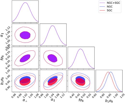
Posterior contour FS for the combined NGC + SGC where the b1σ8 is dependent of the galactic cap.

Figure 11.

Posterior contour FS for the combined NGC + SGC where the b₁σ₈ is dependent of the galactic cap.

Table 10.

Summary of the results on the Hubble distance D_H/r_drag, the transverse comoving diameter distance D_M/r_drag, and of the linear growth rate of structure fσ₈. The quoted error is the quadratic sum of the statistical (standard deviation of chains) and systematic errors. The (OR) line shows the results with a fiducial cosmology being the cosmology used for the OuterRim box, see equation (20).

	D_H/r_drag	D_M/r_drag	fσ₈
DR16	13.52 ± 0.51	30.68 ± 0.90	0.476 ± 0.047
DR16 (OR)	13.81 ± 0.52	30.99 ± 0.92	0.477 ± 0.045
DR14	12.8 ± 0.9	31.0 ± 1.8	0.425 ± 0.077
Error ratio	1.8	2	1.7

	D_H/r_drag	D_M/r_drag	fσ₈
DR16	13.52 ± 0.51	30.68 ± 0.90	0.476 ± 0.047
DR16 (OR)	13.81 ± 0.52	30.99 ± 0.92	0.477 ± 0.045
DR14	12.8 ± 0.9	31.0 ± 1.8	0.425 ± 0.077
Error ratio	1.8	2	1.7

Table 10.

Summary of the results on the Hubble distance D_H/r_drag, the transverse comoving diameter distance D_M/r_drag, and of the linear growth rate of structure fσ₈. The quoted error is the quadratic sum of the statistical (standard deviation of chains) and systematic errors. The (OR) line shows the results with a fiducial cosmology being the cosmology used for the OuterRim box, see equation (20).

	D_H/r_drag	D_M/r_drag	fσ₈
DR16	13.52 ± 0.51	30.68 ± 0.90	0.476 ± 0.047
DR16 (OR)	13.81 ± 0.52	30.99 ± 0.92	0.477 ± 0.045
DR14	12.8 ± 0.9	31.0 ± 1.8	0.425 ± 0.077
Error ratio	1.8	2	1.7

	D_H/r_drag	D_M/r_drag	fσ₈
DR16	13.52 ± 0.51	30.68 ± 0.90	0.476 ± 0.047
DR16 (OR)	13.81 ± 0.52	30.99 ± 0.92	0.477 ± 0.045
DR14	12.8 ± 0.9	31.0 ± 1.8	0.425 ± 0.077
Error ratio	1.8	2	1.7

To test that the results do not depend on the assumed fiducial cosmology, the complete analysis is also done using the OuterRim cosmology as the fiducial cosmology. The results are in agreement, and the observed differences are comparable with what is calculated from the approximate mocks. The effect of the fiducial cosmology is already included in the systematic errors arising from the modelling as studied in the mock challenge (Smith et al. 2020), and we do not quote an additional systematic error from the fiducial cosmology at this stage.

The measurement of the linear growth rate of structures is given in terms of fσ₈ and for the linear power spectrum used in the present analysis, we have σ₈ = 0.401. It is proposed in Gil-Marín et al. (2020) to use the isotropic dilation scale |$\alpha _{\rm iso}=(\alpha _{\parallel }^2\alpha _{\perp })^{1/3}$| to calculate σ₈ in the cosmology implied by the data. This would decrease our measurement of fσ₈ by 2.1 per cent that is close to the systematic error quoted for this parameter. But changes of cosmologies that could lead to such an effect have already been included in the determination of the systematic errors arising from the modelling. Correcting σ₈ should in principle also be applied to the mock challenge and would reduce the systematic error, but we leave this for further work. In another approach, Sanchez (2020) proposes to use σ₁₂ where fluctuations of the linear power spectrum are calculated in spheres of 12 |$\, \mathrm{Mpc}$| instead of 8 |$\, \mathrm{h}^{-1}\mathrm{Mpc}$|⁠. Given the value of h = 0.676 of the fiducial cosmology, the numerical value of σ₁₂ is only 0.8 per cent smaller than σ₈. For completeness, results using this approach are given in appendix D of Hou et al. (2020).

Our results are also compared to those obtained for the Fourier Space analysis of the eBOSS quasar sample from an earlier data release (DR14 Gil-Marín et al. 2018). The interpretation performed in this previous analysis used a different definition of the effective redshift yielding z_eff = 1.52. We recalculate the cosmological parameters D_H(z_eff)/r_drag and D_M(z_eff)/r_drag for the DR14 results using our estimate of the effective redshift (z_eff = 1.480) and we assume that the two samples have the same redshift distribution. The results, given in Table 10, show that the results of the two analyses are statistically compatible at 1-sigma level and that the errors are improved by a factor of 2 for each cosmological parameter using the new data.

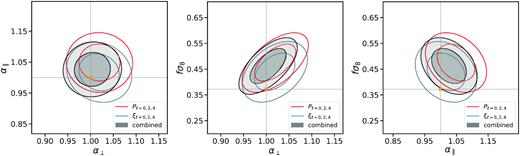
The 2D contours of the posterior for |$\alpha _{\parallel }$| and α_⊥ from the Full-Shape RSD analysis are also compared to the contours obtained for the BAO-only analysis (Fig. 12). The agreement for α_⊥ (resp. |$\alpha _{\parallel }$|⁠) is within 1/10 (resp. 1/2) of the statistical error.

Figure 12.

Posterior contours for the BAO (blue) and FS (red) analysis determined with the MCMC chains.

4.3.4 Consensus

We perform a consensus analysis of our results with the results obtained in configuration space by Hou et al. (2020). The method is based on the work of Sánchez et al. (2017) and is described in section 7.3 of Hou et al. (2020). In this method, a full 6 × 6 covariance matrix is built from the 3 × 3 covariance matrices of the 2-point correlation function and of the power spectrum measurements, and the cross-terms are determined using the 1000 approximate mocks. The observational systematic errors are added in quadrature to the covariance and we consider that they are independent. The modelling systematic error is determined from the mock challenge, where the consensus technique was applied to each mock realization and is found to be smaller than either the configuration or Fourier Space systematic errors. The results are summarized in Table 11 and the posterior contours derived from the MCMC analysis for α_⊥, |$\alpha _{\parallel }$| and fσ₈ are represented in Fig. 13. The measurements are in agreement, and the gain in precision from the consensus is modest. The measurements of |$\alpha _{\parallel }$| and α_⊥ are found to be within 1 σ of a flat ΛCDM model using the cosmological parameters of the combined CMB + BAO measurement of Planck Collaboration VI (2020). Our result of fσ₈ is 1.9 σ above the Planck-derived value.

$Posterior for α⊥, $\alpha _{\parallel }$ and fσ8 configuration space, Fourier Space, and the combined results using the method described in Sánchez et al. (2017). The filled contours are derived from MCMC chains for configuration space (blue) and k-space (red). The black solid ellipses are the combined constraints at 68, 95 confidence limit. The orange crosses denote the values that are inferred from the combined Planck 2018 (Planck Collaboration VI 2020).$

Figure 13.

Posterior for α_⊥, |$\alpha _{\parallel }$| and fσ₈ configuration space, Fourier Space, and the combined results using the method described in Sánchez et al. (2017). The filled contours are derived from MCMC chains for configuration space (blue) and k-space (red). The black solid ellipses are the combined constraints at 68, 95 confidence limit. The orange crosses denote the values that are inferred from the combined Planck 2018 (Planck Collaboration VI 2020).

Table 11.

Final results of the Full-Shape analyses in Fourier and configuration spaces and their consensus.

	D_H(z_eff)/r_drag	D_M(z_eff)/r_drag	fσ₈
Fourier Space	13.52 ± 0.51	30.68 ± 0.90	0.476 ± 0.047
Configuration space	13.11 ± 0.52	30.66 ± 0.88	0.439 ± 0.048
Full-Shape consensus	13.23 ± 0.47	30.21 ± 0.79	0.462 ± 0.045

	D_H(z_eff)/r_drag	D_M(z_eff)/r_drag	fσ₈
Fourier Space	13.52 ± 0.51	30.68 ± 0.90	0.476 ± 0.047
Configuration space	13.11 ± 0.52	30.66 ± 0.88	0.439 ± 0.048
Full-Shape consensus	13.23 ± 0.47	30.21 ± 0.79	0.462 ± 0.045

Table 11.

Final results of the Full-Shape analyses in Fourier and configuration spaces and their consensus.

	D_H(z_eff)/r_drag	D_M(z_eff)/r_drag	fσ₈
Fourier Space	13.52 ± 0.51	30.68 ± 0.90	0.476 ± 0.047
Configuration space	13.11 ± 0.52	30.66 ± 0.88	0.439 ± 0.048
Full-Shape consensus	13.23 ± 0.47	30.21 ± 0.79	0.462 ± 0.045

	D_H(z_eff)/r_drag	D_M(z_eff)/r_drag	fσ₈
Fourier Space	13.52 ± 0.51	30.68 ± 0.90	0.476 ± 0.047
Configuration space	13.11 ± 0.52	30.66 ± 0.88	0.439 ± 0.048
Full-Shape consensus	13.23 ± 0.47	30.21 ± 0.79	0.462 ± 0.045

5 CONCLUSIONS

We perform the analysis of the clustering of the complete eBOSS quasar sample. We did two separate analyses. The BAO-only analysis measures the ratio between the angular diameter distance and the sound horizon at the baryon drag epoch, and the ratio between the Hubble distance and the sound horizon at the baryon drag epoch. The Full-Shape RSD analysis provides in addition a determination of the linear growth rate of structure times the amplitude of matter density fluctuations. We use a dedicated mock challenge (Smith et al. 2020) to estimate the systematic errors due to the modelling of the power spectrum and due to the dependence on the assumed fiducial cosmology. The errors due to the observational systematics are determined from approximate mocks where the observational effects have been modelled. For both methods, the dominant source of systematic error resides in the modelling of the power spectrum. The modelling of fibre collisions also has a large impact on the cosmological parameters, especially on the growth rate measurement. The overall systematic errors are at the level of 30 per cent of the statistical errors. Therefore, improving the models is key for the next-generation quasar surveys with increased statistics. A consensus analysis of our measurement in Fourier Space and the measurement in configuration space from Hou et al. (2020) give the following constraints for the BAO-only analysis:

$$\begin{eqnarray*} D_{\rm H}/r_{\rm drag} = \frac{c}{Hr_{\rm drag}} &=& 13.26 \pm 0.55 \nonumber \\ D_{\rm M}/r_{\rm drag} &=& 30.69 \pm 0.80 , \end{eqnarray*}$$

(41)

and for the Full-Shape RSD analysis, it yields:

$$\begin{eqnarray*} D_{\rm H}/r_{\rm drag} &=&13.23 \pm 0.47 \nonumber \\ D_{\rm M}/r_{\rm drag} &=&30.21 \pm 0.79 \nonumber \\ f\sigma _8 &=&0.462 \pm 0.045 . \end{eqnarray*}$$

(42)

These measurements are proven very robust by all tests performed. Our measurements of cosmological distances are in agreement with a flat ΛCDM model using Planck Collaboration VI (2020) and our measurement of the linear growth of structures, fσ₈, is 1.9 σ above the Planck-derived value. The cosmological interpretation of the DR16 eBOSS quasar sample measurement along with the measurements obtained for the other eBOSS tracers and the consistency with external data sets are discussed in eBOSS Collaboration (2020).

ACKNOWLEDGEMENTS

R. Neveux acknowledges support from grant ANR-16-CE31-0021, eBOSS and from ANR-17-CE31-0024-01, NILAC. Funding for SDSS-III and SDSS-IV has been provided by the Alfred P. Sloan Foundation and participating institutions. Additional funding for SDSS-III comes from the National Science Foundation and the U.S. Department of Energy Office of Science. Further information about both projects is available at www.sdss.org. SDSS is managed by the Astrophysical Research Consortium for the Participating Institutions in both collaborations. In SDSS-III, these include the University of Arizona, the Brazilian Participation Group, Brookhaven National Laboratory, Carnegie Mellon University, University of Florida, the French Participation Group, the German Participation Group, Harvard University, the Instituto de Astrofisica de Canarias, the Michigan State/Notre Dame/JINA Participation Group, Johns Hopkins University, Lawrence Berkeley National Laboratory, Max Planck Institute for Astrophysics, Max Planck Institute for Extraterrestrial Physics, New Mexico State University, New York University, Ohio State University, Pennsylvania State University, University of Portsmouth, Princeton University, the Spanish Participation Group, University of Tokyo, University of Utah, Vanderbilt University, University of Virginia, University of Washington, and Yale University. The Participating Institutions in SDSS-IV are Carnegie Mellon University, Colorado University, Boulder, Harvard-Smithsonian Center for Astrophysics Participation Group, Johns Hopkins University, Kavli Institute for the Physics and Mathematics of the Universe Max-Planck-Institut fuer Astrophysik (MPA Garching), Max-Planck-Institut fuer Extraterrestrische Physik (MPE), Max-Planck-Institut fuer Astronomie (MPIA Heidelberg), National Astronomical Observatories of China, New Mexico State University, New York University, The Ohio State University, Penn State University, Shanghai Astronomical Observatory, United Kingdom Participation Group, University of Portsmouth, University of Utah, University of Wisconsin, and Yale University. This research used resources of the Argonne Leadership Computing Facility, which is a DOE Office of Science User Facility supported under contract DE- AC02-06CH11357. This work made use of the facilities and staff of the UK Sciama High Performance Computing cluster supported by the ICG, SEPNet, and the University of Portsmouth. This research used resources of the National Energy Research Scientific Computing Center, a DOE Office of Science User Facility supported by the Office of Science of the U.S. Department of Energy under contract no. DE-AC02-05CH11231.

DATA AVAILABILITY

The power spectrum, covariance matrices, and resulting likelihoods for cosmological parameters are (will be made) available (after acceptance) via the SDSS Science Archive Server (https://sas.sdss.org/), with the exact address tbd.

Footnotes

1

A summary of all SDSS BAO and RSD measurements with accompanying legacy figures can be found here: https://www.sdss.org/science/final-bao-and-rsd-measurements/. The full cosmological interpretation of these measurements can be found here: https://www.sdss.org/science/cosmology-results-from-eboss/

2

MINUIT, Function Minimization and Error analysis, James F., CERN 1994.

REFERENCES

Alam

S.

et al. ,

2017

,

MNRAS

,

470

,

2617

10.1093/mnras/stx721

Alcock

C.

,

Paczynski

B.

,

1979

,

Nature

,

281

,

358

10.1038/281358a0

10.1111/j.1365-2966.2010.16459.x

Angulo

R. E.

,

White

S. D. M.

,

2010

,

MNRAS

,

405

,

143

Ata

M.

et al. ,

2018

,

MNRAS

,

473

,

4773

10.1093/mnras/stx2630

Bautista

J. E.

et al. ,

2018

,

ApJ

,

863

,

110

10.3847/1538-4357/aacea5

Bautista

J. E.

et al. ,

2020

,

MNRAS

,

in press

10.1093/mnras/staa2800

Beutler

F.

et al. ,

2016

,

MNRAS

,

464

,

3409

10.1093/mnras/stw2373

10.1088/1475-7516/2019/03/040

Beutler

F.

,

Castorina

E.

,

Zhang

P.

,

2019

,

J. Cosmol. Astropart. Phys.

,

2019

,

040

Bianchi

D.

,

Gil-Marín

H.

,

Ruggeri

R.

,

Percival

W. J.

,

2015

,

MNRAS

,

453

,

L11

10.1093/mnrasl/slv090

Blanton

M. R.

,

Lin

H.

,

Lupton

R. H.

,

Maley

F. M.

,

Young

N.

,

Zehavi

I.

,

Loveday

J.

,

2003

,

AJ

,

125

,

2276

10.1086/344761

Blanton

M. R.

et al. ,

2017

,

AJ

,

154

,

28

10.3847/1538-3881/aa7567

10.1088/0004-637X/729/2/141

Bovy

J.

et al. ,

2011

,

ApJ

,

729

,

141

Chuang

C.-H.

,

Kitaura

F.-S.

,

Prada

F.

,

Zhao

C.

,

Yepes

G.

,

2015

,

MNRAS

,

446

,

2621

10.1093/mnras/stu2301

10.1111/j.1365-2966.2005.09318.x

Cole

S.

et al. ,

2005

,

MNRAS

,

362

,

505

10.1111/j.1365-2966.2008.14052.x

Croom

S. M.

et al. ,

2009

,

MNRAS

,

392

,

19

10.3847/0004-6256/151/2/44

Dawson

K. S.

et al. ,

2016

,

AJ

,

151

,

44

10.1088/1475-7516/2019/08/036

de Mattia

A.

,

Ruhlmann-Kleider

V.

,

2019

,

J. Cosmol. Astropart. Phys.

,

2019

,

036

de Mattia

A.

et al. ,

2020

,

preprint (arXiv:2007.09008)

du Mas des Bourboux

H.

et al. ,

2020

,

preprint (arXiv:2007.08995)

eBOSS Collaboration

,

2020

,

preprint (arXiv:2007.08991)

Eftekharzadeh

S.

et al. ,

2015

,

MNRAS

,

453

,

2779

10.1093/mnras/stv1763

Eisenstein

D. J.

et al. ,

2005

,

ApJ

,

633

,

560

10.1086/466512

Feldman

H. A.

,

Kaiser

N.

,

Peacock

J. A.

,

1994

,

ApJ

,

426

,

23

10.1086/174036

Foreman-Mackey

D.

,

Hogg

D. W.

,

Lang

D.

,

Goodman

J.

,

2013

,

PASP

,

125

,

306

10.1086/670067

Fukugita

M.

,

Ichikawa

T.

,

Gunn

J. E.

,

Doi

M.

,

Shimasaku

K.

,

Schneider

D. P.

,

1996

,

AJ

,

111

,

1748

10.1086/117915

Gil-Marín

H.

et al. ,

2018

,

MNRAS

,

477

,

1604

10.1093/mnras/sty453

Gil-Marín

H.

et al. ,

2020

,

preprint (arXiv:2007.08994)

Gunn

J. E.

et al. ,

2006

,

AJ

,

131

,

2332

10.1086/500975

10.1016/j.newast.2015.06.003

Habib

S.

et al. ,

2016

,

New Astron.

,

42

,

49

Hahn

C.

,

Scoccimarro

R.

,

Blanton

M. R.

,

Tinker

J. L.

,

Rodríguez-Torres

S. A.

,

2017

,

MNRAS

,

467

,

1940

10.1093/mnras/stx185

10.1088/1475-7516/2017/07/002

Hand

N.

,

Li

Y.

,

Slepian

Z.

,

Seljak

U.

,

2017

,

J. Cosmol. Astropart. Phys.

,

2017

,

002

Hand

N.

,

Feng

Y.

,

Beutler

F.

,

Li

Y.

,

Modi

C.

,

Seljak

U.

,

Slepian

Z.

,

2018

,

AJ

,

156

,

160

10.3847/1538-3881/aadae0

10.1051/0004-6361:20066170

Hartlap

J.

,

Simon

P.

,

Schneider

P.

,

2007

,

A&A

,

464

,

399

Hinton

S. R.

,

Howlett

C.

,

Davis

T. M.

,

2020

,

MNRAS

,

493

,

4078

10.1093/mnras/staa361

Hou

J.

et al. ,

2018

,

MNRAS

,

480

,

2521

10.1093/mnras/sty1984

Hou

J.

et al. ,

2020

,

preprint (arXiv:2007.08998)

Hu

W.

,

Sugiyama

N.

,

1995

,

Phys. Rev. D

,

51

,

2599

10.1103/PhysRevD.51.2599

Kaiser

N.

,

1987

,

MNRAS

,

227

,

1

10.1093/mnras/227.1.1

Karagiannis

D.

,

Shanks

T.

,

Ross

N. P.

,

2014

,

MNRAS

,

441

,

486

10.1093/mnras/stu590

10.1088/1475-7516/2013/03/024

Kirkby

D.

et al. ,

2013

,

J. Cosmol. Astropart. Phys.

,

2013

,

024

10.1088/0067-0049/192/2/18

Komatsu

E.

et al. ,

2011

,

ApJS

,

192

,

18

10.1088/1475-7516/2016/11/060

Laurent

P.

et al. ,

2016

,

J. Cosmol. Astropart. Phys.

,

11

,

060

10.1016/j.astropartphys.2007.09.003

Linder

E. V.

,

Cahn

R. N.

,

2007

,

Astropart. Phys.

,

28

,

481

Lyke

B. W.

et al. ,

2020

,

ApJS

,

250

,

8

10.3847/1538-4365/aba623

10.1088/1475-7516/2009/08/020

McDonald

P.

,

Roy

A.

,

2009

,

J. Cosmol. Astropart. Phys.

,

2009

,

020

Mead

A. J.

,

Peacock

J. A.

,

2014

,

MNRAS

,

440

,

1233

10.1093/mnras/stu345

Mohammad

F. G.

et al. ,

2020

,

MNRAS

,

498

,

128

10.1093/mnras/staa2344

Myers

A. D.

,

Brunner

R. J.

,

Nichol

R. C.

,

Richards

G. T.

,

Schneider

D. P.

,

Bahcall

N. A.

,

2007

,

ApJ

,

658

,

85

10.1086/511519

10.1088/0067-0049/221/2/27

Myers

A. D.

et al. ,

2015

,

ApJS

,

221

,

27

Navarro

J. F.

,

Frenk

C. S.

,

White

S. D. M.

,

1996

,

ApJ

,

462

,

563

10.1086/177173

Percival

W. J.

,

Bianchi

D.

,

2017

,

MNRAS

,

472

,

L40

10.1093/mnrasl/slx135

10.1111/j.1365-2966.2008.14211.x

Percival

W. J.

,

White

M.

,

2009

,

MNRAS

,

393

,

297

Percival

W. J.

et al. ,

2014

,

MNRAS

,

439

,

2531

10.1093/mnras/stu112

10.1051/0004-6361/201833910

Planck Collaboration VI

,

2020

,

A&A

,

641

,

A6

10.1111/j.1365-2966.2012.21235.x

Raichoor

A.

et al. ,

2020

,

preprint (arXiv:2007.09007)

Ross

A. J.

et al. ,

2012

,

MNRAS

,

424

,

564

Ross

A. J.

,

Percival

W. J.

,

Manera

M.

,

2015

,

MNRAS

,

451

,

1331

10.1093/mnras/stv966

Ross

A. J.

et al. ,

2020

,

MNRAS

,

498

,

2354

10.1093/mnras/staa2416

10.1088/0004-637X/697/2/1634

Ross

N. P.

et al. ,

2009

,

ApJ

,

697

,

1634

Sanchez

A. G.

,

2020

,

preprint (arXiv:2002.07829)

Sánchez

A. G.

et al. ,

2017

,

MNRAS

,

464

,

1493

10.1093/mnras/stw2495

Scolnic

D. M.

et al. ,

2018

,

ApJ

,

859

,

101

10.3847/1538-4357/aab9bb

Sefusatti

E.

,

Crocce

M.

,

Scoccimarro

R.

,

Couchman

H. M. P.

,

2016

,

MNRAS

,

460

,

3624

10.1093/mnras/stw1229

10.1088/0004-637X/697/2/1656

Shen

Y.

et al. ,

2009

,

ApJ

,

697

,

1656

10.1088/0004-6256/146/2/32

Smee

S. A.

et al. ,

2013

,

AJ

,

146

,

32

Smith

A.

et al. ,

2020

,

MNRAS

,

in press

10.1093/mnras/staa2825

10.1103/PhysRevD.82.063522

Tamone

A.

et al. ,

2020

,

preprint (arXiv:2007.09009)

Taruya

A.

,

2014

,

Astrophysics Source Code Library, record ascl:1404.012

Taruya

A.

,

Nishimichi

T.

,

Saito

S.

,

2010

,

Phys. Rev. D

,

82

,

063522

10.1111/j.1365-2966.2012.21251.x

White

M.

et al. ,

2012

,

MNRAS

,

424

,

933

10.1088/0004-6256/140/6/1868

Wright

E. L.

et al. ,

2010

,

AJ

,

140

,

1868

Yamamoto

K.

,

Nakamichi

M.

,

Kamino

A.

,

Bassett

B. A.

,

Nishioka

H.

,

2006

,

PASJ

,

58

,

93

10.1093/pasj/58.1.93

Zarrouk

P.

et al. ,

2018

,

MNRAS

,

477

,

1639

10.1093/mnras/sty506

Zhao

C.

et al. ,

2020

,

preprint (arXiv:2007.08997)

APPENDIX A: POSTERIOR DISTRIBUTIONS DERIVED FROM THE MCMC ANALYSIS

In this appendix, we provide the full 68 per cent and 95 per cent confidence-level contours and Gaussian approximation for all parameters used in the Full-Shape RSD analysis. In Fig. A1 (resp. Fig. A2), we show the contours for the cosmological parameters and for the nuisance parameters of Northern (resp. Southern) galactic caps. Fig. A3 shows the contours of the NGC and SGC nuisance parameters. As stated in the main part of this paper, the contours involving cosmological parameters are found to be Gaussian. For the nuisance parameters, we observe that all contours involving the quasar count stochastic term A_g presented in Section 4 are not Gaussian, and that there is strong degeneracy between A_g and the second-order bias b₂ for both the NGC and the SGC.

Figure A1.

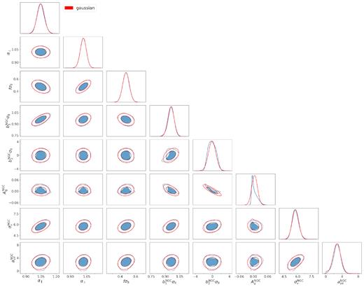
68 per cent and 95 per cent confidence-level contours (blue) and Gaussian approximation (red) for the cosmological parameters and for the NGC nuisance parameters described in Table 6.

Figure A2.

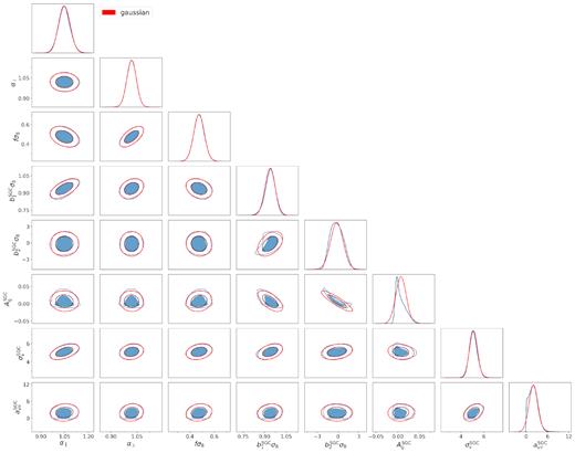
68 per cent and 95 per cent confidence-level contours (blue) and Gaussian approximation (red) for the cosmological parameters and for the SGC nuisance parameters described in Table 6.

Figure A3.

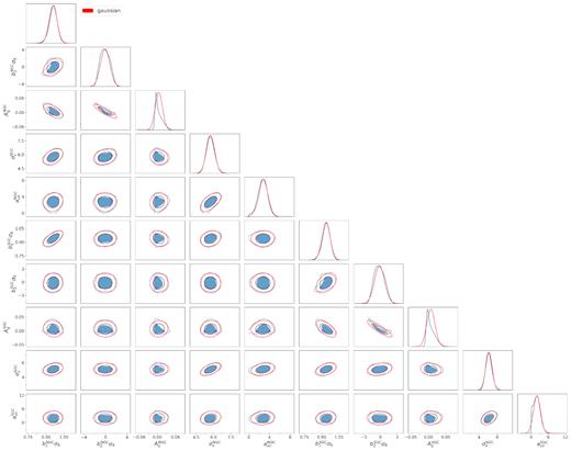
68 per cent and 95 per cent confidence-level contours (blue) and Gaussian approximation (red) for the NGC and SGC nuisance parameters described in Table 6.