


ABSTRACT
We present 2000 mock galaxy catalogues for the analysis of baryon acoustic oscillations (BAOs) in the Emission Line Galaxy (ELG) sample of the extended Baryon Oscillation Spectroscopic Survey Data Release 16 (eBOSS DR16). Each mock catalogue has a number density of |$6.7 \times 10^{-4} h^3 \rm Mpc^{-3}$|, covering a redshift range from 0.6 to 1.1. The mocks are calibrated to small-scale eBOSS ELG clustering measurements at scales of |$\lesssim 30\, h^{-1}$|Mpc. The mock catalogues are generated using a combination of GaLAxy Mocks (GLAM) simulations and the quick particle-mesh (QPM) method. GLAM simulations are used to generate the density field, which is then assigned dark matter haloes using the QPM method. Haloes are populated with galaxies using a halo occupation distribution. The resulting mocks match the survey geometry and selection function of the data, and have slightly higher number density that allows room for systematic analysis. The large-scale clustering of mocks at the BAO scale is consistent with data and we present the correlation matrix of the mocks.
1 INTRODUCTION
In modern cosmology, the study of the large-scale structure (LSS) provides key information about the expansion history and growth of structure in the Universe (Davis & Peebles 1983; Eisenstein et al. 2005). Measurements of baryon acoustic oscillations (BAO; Eisenstein & Hu 1998) and redshift-space distortions (RSD; Kaiser 1987) require spectroscopic surveys to cover large volumes and to have accurate redshift measurements. In the past, large redshift surveys have included 2dFGRS (Cole et al. 2005), the Sloan Digital Sky Survey (SDSS-II; Eisenstein et al. 2005), 6dFGRS (Beutler et al. 2012), WiggleZ (Blake et al. 2011), and SDSS-III Baryon Oscillation Spectroscopic Survey (BOSS; Dawson et al. 2013). The recently completed extended Baryon Oscillation Spectroscopic Survey (eBOSS; Dawson et al. 2016) is a five year program of the Sloan Sky Digital Survey (SDSS-IV; Blanton et al. 2017) and is aiming at measuring the distance–redshift relation with BAO at the per cent-level using various galaxy tracers.
One important question for big redshift surveys is how to determine the uncertainties in the measurements of cosmological parameters. Simulated mock catalogues can be used to estimate the covariance matrix of galaxy clustering and these errors are propagated to cosmological parameter uncertainties by integrating over the parameter likelihood function (Dodelson & Schneider 2013; Percival et al. 2014). This method requires accurate mock catalogues to cover a huge volume and large number density of galaxies as the survey geometry and redshift range grow larger. Determining the uncertainties of a large survey such as eBOSS requires thousands of mock catalogues, which can be computationally expensive. In recent years, several quick methods such as quick particle mesh (QPM; White, Tinker & McBride 2014), effective Zel’dovich approximation (EZmocks; Chuang et al. 2015), and PerturbAtion Theory Catalog generator of Halo and galaxY distributions (PATCHY; Kitaura, Yepes & Prada 2014) have been developed to generate mocks efficiently. EZmocks use an ad hoc model to populate galaxies directly on the dark matter field that is generated using the Zeldovich approximation. A similar approach is used by PATCHY but using Augmented Lagrangian Perturbation Theory instead, while the QPM method selects dark matter particles that mimic the statistics of dark matter haloes, and then populate galaxies in dark matter haloes using a standard halo occupation approach.
We present a set of mock catalogues for the eBOSS ELG sample, which have been tuned to reproduce the small-scale clustering measurements. In this work, we focus on the ELG sample in the 0.6 < z < 1.1 redshift range. ELGs present a unique challenge for error estimation. These galaxies typically lie in low-mass haloes but can be mapped to very large volumes. Thus, even producing a single N-body simulation that properly resolves ELG haloes but covers an appropriate volume is a challenge. To circumvent this problem, we use the GLAM N-body simulations (Klypin & Prada 2018) and the QPM method to construct the ersatz halo catalogues. Galaxies are then populated using the halo occupation distribution (HOD) model to match the two-point statistics of the eBOSS ELG measurements. We produce a set of 2000 accurate mock catalogues for the estimation of the covariance matrix. The mock catalogues are calibrated to match the ELG clustering at 10 h−1Mpc scales.
This study is part of a series of papers of the final eBOSS DR16 data and cosmological measurements. The BAO and RSD results are presented in Bautista et al. (2020) and Gil-Marin et al. (2020) for luminous red galaxies (LRGs); for emission line galaxies (ELGs) see Raichoor (2020), Tamone et al. (2020), and de Mattia (2020); and see Hou et al. (2020) and Neveux et al. (2020) for quasars. The essential data catalogues are presented in Ross et al. (2020) and Lyke et al. (2020), the N-body mocks for systematic errors are presented in Rossi et al. (2020) and Smith et al. (2020), another set of approximate mocks is presented in Zhao et al. (2020). The ELG mock challenge result is presented in Alam et al. (2020), the ELG HOD analysis is presented in Avila et al. (2020). The measurements of BAO in the Lyα forest is presented in du Mas des Bourboux et al. (2020). The mock catalogues produced in this paper are utilized in the BAO and growth-of-structure analysis of the ELG sample in de Mattia (2020). Lastly, the cosmological interpretation of the full eBOSS sample can be found in Collaboration et al. (2020).
This paper is organized as follows: Section 2 describes the eBOSS ELG sample used in the analysis. In Section 3, we present our small-scale clustering measurements, with systematic corrections, that we use to calibrate our mock catalogues. The procedure of creating mock catalogues is described in Section 4. Section 5 compares the large-scale clustering of the ELG sample and GLAM-QPM mocks, and we present the covariance matrix. Finally we discuss our results in Section 6. In this paper, the distances are measured in units of h−1Mpc with the Hubble constant |$H_0=100h \text {km s}^{-1}\text {Mpc}^{-1}$|. We assume a fiducial ΛCDM cosmology with parameters (Ωm, h, Ωbh2, σ8, ns) = (0.307, 0.678, 0.022, 0.828, 0.96) for the redshift–distance relationship and mock catalogue generation.
2 DATA
The eBOSS survey was conducted using the Sloan Foundation 2.5-m Telescope at Apache Point Observatory (Gunn et al. 2006) to conduct spectroscopic observations. It used the same 1000-fibre spectrographs as BOSS (Smee et al. 2013) to measure four tracers of the underlying dark matter density field. In data release 16, the survey has measured accurate redshifts of 174 816 LRGs in the redshift range 0.6 < z < 1.0 (Ross et al. 2020), 173 736 ELGs in the redshift range 0.6 < z < 1.1 (Raichoor 2020), 343 708 quasars within 0.8 < z < 2.2 (Lyke et al. 2020; Ross et al. 2020), and 210 005 Lyα quasars within z > 2.1 (du Mas des Bourboux et al. 2020). Overall these data sets constrain the redshift–distance relation to 1–3 per cent level at 4 redshifts (Dawson et al. 2016; Collaboration et al. 2020).
The eBOSS/ELG program started in September 2016 and it is the first time ELG tracers have been used in SDSS for large-scale clustering measurements. Preliminary work tested the feasibility of using the BOSS spectrograph to conduct ELG observations (Comparat et al. 2013) and the reliability of redshift measurements (Comparat et al. 2015, 2016). The ELG target selection (Raichoor et al. 2017) uses the DECam Legacy Survey (DECaLS; Dey et al. 2018). Its deep imaging data provides the opportunity to reach higher redshift and higher efficiency, defined aspercentage of observed ELGs having reliable zspec (Raichoor et al. 2017). The eBOSS/ELG footprint covers an effective area of 369.5 deg2 in the north galactic cap (NGC) and 357.5 deg2 in the south galactic cap (SGC), with an overall number density of 313.0 deg−2 (Raichoor 2020).
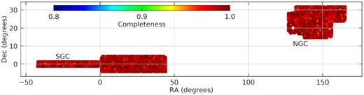
The footprint of the ELG SGC and NGC survey, where the colour represents the completeness in each sector. The mean completeness in each sector is 0.9909 for NGC and 0.9906 for SGC. Gaps and variations in the completeness maps are due to tiles that could not be observed, or locations in the footprint where tiles did not overlap. See Raichoor (2020) for details.
3 GALAXY CLUSTERING
Galaxies are not randomly distributed in the Universe. Density perturbations, which are created in the early Universe, evolve under gravitational attraction, and are the seeds of the LSS we see today. In this paper, we study the statistics of the ELG galaxy distribution in the eBOSS survey using the two-point correlation function, ξ(r) = 〈δ(x)δ(x + r)〉, which is a measure of the excess probability of finding a pair of galaxies, separated by a distance r, compared to if the galaxies were distributed randomly (Peebles 1980). Measurements of clustering on large scales allow us to constrain cosmological parameters via measuring the position of BAO peak and the shape of the clustering signal. On small scales, clustering measurements can be used to probe the relationship between galaxy properties and dark matter haloes. At scales |$\gtrsim 30\, h^{-1}$| Mpc, clustering is more sensitive to systematic errors in the imaging, while carrying less information about galaxy-halo connection. Thus, we focus on small-scale clustering to calibrate the adopted HOD model to generate the ELG mocks. We will discuss the HOD model further in Section 4.3.
The systematic weights, wsys, are calculated by using a linear fit of the ELG target density in various photometric variables: galactic extinction, stellar density, H i density, grz-band image seeing, and grz-band image depth (Raichoor 2020). The close-pair weights, wcp, are calculated by upweighting galaxies in collided pairs by coefficient Ntarget/Nfibre, where Ntarget is the total number of targets in the collision group and Nfibre is the number of targets in the collision group that has been assigned fibres. The redshift failure weights, wnoz, are the inverse of two fitting functions to the plate-averaged signal-to-noise ratio (pSN) and the fibre position in the focal plane. Details of the systematic model is described in the eBOSS ELG catalogue paper (Raichoor 2020).
Fig. 2 presents our results of the small-scale clustering from 0.34 to |$70\,h^{-1}\,\rm Mpc$| in 12 logarithmic bins, after applying the weighting described above. The lower limit is set by shot noise in the pair counts. We refer to these data as ‘small-scale’ to separate them from clustering at the BAO scale. The SGC and NGC are divided into 25 roughly equal spherical areas and the errors are estimated using the jackknife resampling technique. There is no significant difference seen between the clustering of the SGC and NGC. We refer to these data as small-scale clustering to separate them from clustering at the BAO scale.
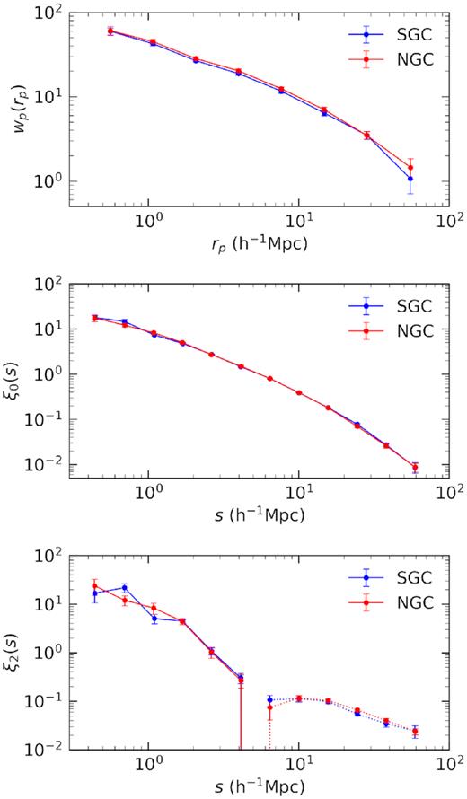
Projected correlation function, wp (upper panel), redshift-space monopole, ξ0 (middle panel), and quadrupole, ξ2 (lower panel) for ELGs in the SGC (blue) and NGC (red). Correlation functions are shown for separations between 0.3 and |$70\,h^{-1}\,\rm Mpc$|, for ELGs in the redshift range 0.6 < z < 1.1. Dotted curves in the lower panel indicate negative values. The errorbars are estimated using jackknife resampling, with 25 jackknife samples.
4 MOCK GENERATION
In order to construct accurate mocks to interpret the ELG clustering, we combine GaLAxy Mocks (GLAM) simulations with the quick particle-mesh (QPM) scheme. The whole process can be summarized in the following steps:
In the first step, we run 2000 large GLAM N-body simulations with box size of |$3000\, h^{-1}\,\rm {Mpc}$|. This box size is large enough to cover the whole footprint of ELGs up to redshift z = 1.1.
In the second step, we apply the QPM code to assign dark matter haloes within the density field of the GLAM simulations.
In the third step, we populate the haloes with galaxies using an HOD model that is calibrated to reproduce the small-scale clustering measurements of the data.
In the fourth step, we cut the mock catalogues according to the ELG survey geometry. We compare the large-scale clustering of the mocks with the data.
In the next sub-sections, we will describe the details of generating the mock galaxy catalogues.
4.1 GLAM simulations
GLAM (Klypin & Prada 2018) is a new parallel version of the particle-mesh (PM) code that can quickly produce a large number of N-body simulations. We use the GLAM code to generate the matter density field for our mock catalogues since the computational speed is much faster than for QPM simulations. We used MareNostrum-4 computer at Barcelona Supercomputer Center to generate 2000 realizations in the adopted cosmology (see Section 1). The volume of each simulation is |$3\,h^{-1}\,\rm Gpc$|, which is large enough to cover the ELG redshift range 0.6 < z < 1.1. We used 15003 particles with a mass per particle of |$6.8\times 10^{11}h^{-1}\,\rm M_\odot$|. The simulations were started at z = 100 and a constant time-step is used at low redshifts but periodically increases at high redshifts. The total number of time-steps is 94, which is large enough to satisfy both accuracy and stability of the integration of the particle trajectories inside dense regions (Klypin & Prada 2018). Under this set of simulation parameters, the total number of CPU hours is 52 000. In order to make the process as efficient as possible, we incorporate QPM as a module in the GLAM code, so halo catalogue creation is done on the fly. This procedure prevents extra time consumption due to I/O of large files, and saves disk storage.
4.2 From N-body simulation to halo catalogues
There are many benefits to first create halo catalogues and then generate galaxy mocks using galaxy-halo models. One of which is that we can model multiple target samples with different biases within the halo occupation framework. The other advantage is that we can study and test different galaxy-halo models for the same sample.
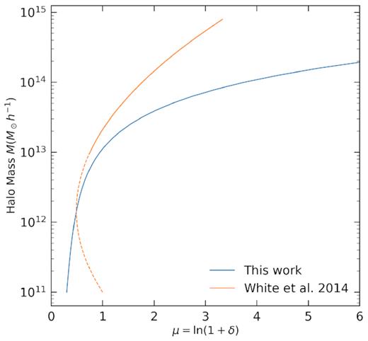
Fitting function describing the relationship between the dark matter overdensity and halo mass, where μ = ln (1 + δ). The fitting function used in this work (blue) is approximately logarithmic approximation at low halo masses, transitioning to a power law at the high halo mass end. For comparison, the mapping used in White et al. (2014) is shown in orange. The scatter of the mapping is 0.1 dex, as described in equation (10). Only haloes with Mh > 1013h−1M⊙ are used in White et al. (2014). The functions differ at high masses since they are for haloes at different redshifts.
Finally, in order to have the correct halo mass function, we divided the halo masses into Nh bins, where the number Nh is large so that the change in b(Mh) between each bin is small. For each mass bin we calculate the number of particles we need to sample to match the mass function n(Mh) of Tinker et al. (2008), then we loop over all particles, assigning particles as haloes with the corresponding probability.
In Fig. 4, we show the average halo mass function from 10 halo catalogues. The 10 catalogues are generated independently from different GLAM simulations. Compared to the QPM mocks used for BOSS LRG sample (Alam et al. 2017), our halo catalogues agree very well to the halo mass function in Tinker et al. (2008) at low halo mass. This verifies that our method yields the correct halo mass function. The small discrepancy at the high halo mass end is due to the power-law formalism we choose for μ(Mh), which means it is less likely to have haloes with mass larger than |$10^{15}\,h^{-1}\,\rm M_\odot$|. Since the fraction of ELGs in haloes with |$M_h\gtrsim 10^{15}\,h^{-1}\,\rm M_\odot$| is negligible, this discrepancy will not have a significant impact on our mocks.
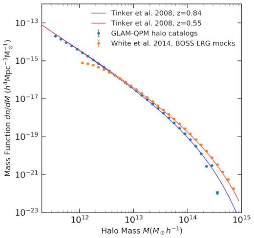
The halo mass function from the GLAM-QPM mocks generated in this work (blue points) compared to BOSS LRG mocks (orange points), which are created using the QPM method (White et al. 2014). For both, we show the average mass function of 10 mocks. The errorbars are the standard deviation among the 10 halo catalogues. As a comparison, we also plot the halo mass function from Tinker et al. (2008) at redshift z = 0.55 (red) and z = 0.84 (blue).
In Fig. 5, we compare the halo bias calculated from the halo catalogues with the halo bias of Tinker et al. (2010). The result are in very good agreement for |$M_h\lt 10^{13.5}\, h^{-1}\, \rm M_\odot$|. The small discrepancy at higher halo mass is due to lack of information of the bias in high-density regions: there is insufficient number of particles that have high density to compute the bias. Considering that the mean halo mass of ELGs is around |$10^{12}\, h^{-1}\, \rm M_\odot$|, this discrepancy should be negligible.
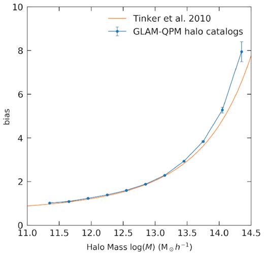
The average halo bias from 10 GLAM-QPM halo catalogues (blue), where the error bars indicate the standard error on the mean. The orange curve indicates the fitting function of Tinker et al. (2010) at redshift z = 0.84.
4.3 Halo occupation distribution for ELGs
We use the HOD to model galaxy bias (Benson et al. 2000; Peacock & Smith 2000; Seljak 2000; Scoccimarro et al. 2001; Berlind & Weinberg 2002; Zheng et al. 2009; White et al. 2011). The HOD formalism describes the relation between a typical class of galaxies and dark matter haloes by the probability P(N|M) that a halo with mass M contains N such galaxies. The population of galaxies can be split into central galaxies, which reside at the centre of the halo, and satellite galaxies. Here, we assume that the satellite galaxies in each halo follow the same radial distribution as the dark matter, corresponding to a NFW profile (Navarro, Frenk & White 1997) where we use the concentration–mass relation of Macciò et al. (2007). The HOD model is a complete description of galaxy bias, i.e. given an HOD model and the halo population from a cosmological model, one can calculate any galaxy clustering statistic on any scale.
This formalism is simplified from previous studies, but it is sufficient to model the ELG clustering. The six free parameters in our HOD model are {fmax, Mmin, σlog M, Mcut, M1, α}. The units of Mmin, M1, and Mcut are |$h^{-1}\, \rm M_\odot$|, while α, fmax, and σlog M are dimensionless quantities. We perform a coarse HOD parameter space search for parameter optimization. A value for each parameter is selected for {Mmin, Mcut, M1, α} while fixing fmax = 0.15 and σlog M = 0.25. There is significant degeneracy between these two parameters and the large-scale galaxy bias. These parameters were chosen to match expected ELG bias as well as meet the expectation that only a minority of haloes would house ELG galaxies in the sample. But these choices prevent the halo occupation model from going significantly below the halo resolution limit of the GLAM-QPM catalogues. The full parameter space is shown in Table 1. In subsequent sections, we will demonstrate that the ELG clustering is relatively insensitive to the choice of parameters. Thus, we did not explore the whole HOD parameter space, which would be out of the scope of this paper. For the purpose of mock generation, our method is sufficient to model the large-scale bias of ELGs, with reasonable choices for the satellite fraction of the target sample.
HOD parameter space for parameter optimization.
| Parameter space | |
|---|---|
| |$M_{\rm min}\, (h^{-1}\,\rm M_\odot)$| | 1.0 × 10¹², 1.5 × 10¹², 2.0 × 10¹² |
| M1|$(h^{-1}\,\rm M_\odot)$| | 2.0 × 10¹³, 5.0 × 10¹³, 8.0 × 10¹³ |
| Mcut|$(h^{-1}\,\rm M_\odot)$| | 7 × 10¹¹, 4 × 10¹² |
| α | 0.8, 1.0, 1.2 |
| Parameter space | |
|---|---|
| |$M_{\rm min}\, (h^{-1}\,\rm M_\odot)$| | 1.0 × 10¹², 1.5 × 10¹², 2.0 × 10¹² |
| M1|$(h^{-1}\,\rm M_\odot)$| | 2.0 × 10¹³, 5.0 × 10¹³, 8.0 × 10¹³ |
| Mcut|$(h^{-1}\,\rm M_\odot)$| | 7 × 10¹¹, 4 × 10¹² |
| α | 0.8, 1.0, 1.2 |
There are 54 sets of parameter in total. For each set, we generate a galaxy mock and measure the redshift-space monopole ξ0(s), quadrupole ξ2(s), as well as projected correlation function wp(rp). We calibrate the HOD by finding the set of parameters which most closely match the clustering of the data at scales between 10 and 30 h−1Mpc, as one would interpret the linear bias at this scale. We also require that the HOD model match the data at <1h−1Mpc, which constraints the fraction of ELGs that are satellite galaxies. At intermediate scales, i.e. s ∼ 1 h−1 Mpc, the QPM scheme does not model the bias well. We will illustrate this point presently. At larger scales, the uncertainty in the clustering measurements from the data is large due to sample variance, and the clustering measurements are more prone to residual photometric systematics. The best-fitting HOD parameters that we use to generate ELG mocks are listed in Table 2. We tested the effect of varying fmax and σlog M, and found that this does not significantly change the clustering measurements.
HOD parameters for our fiducial galaxy mocks.
| Best fit | |
|---|---|
| Mmin | |$1.5\times 10^{12}~ h^{-1}\,\rm M_\odot$| |
| M1 | |$8\times 10^{13}~ h^{-1}\,\rm M_\odot$| |
| Mcut | |$7\times 10^{11}~ h^{-1}\,\rm M_\odot$| |
| α | 1.0 |
| fmax | 0.15 |
| σlog M | 0.25 |
| Best fit | |
|---|---|
| Mmin | |$1.5\times 10^{12}~ h^{-1}\,\rm M_\odot$| |
| M1 | |$8\times 10^{13}~ h^{-1}\,\rm M_\odot$| |
| Mcut | |$7\times 10^{11}~ h^{-1}\,\rm M_\odot$| |
| α | 1.0 |
| fmax | 0.15 |
| σlog M | 0.25 |
The occupation function of central galaxies and satellite galaxies is shown in the upper left panel of Fig. 6. The satellite fraction is |$17.4{{\ \rm per\ cent}}$|, in accordance with |$\sim 20{{\ \rm per\ cent}}$| satellite fraction of star-forming galaxies in Tinker et al. (2013). This is also in agreement with Favole et al. (2016), where it was found that |$22.5\pm 2.5{{\ \rm per\ cent}}$| of ELGs at redshift 0.8 are satellite galaxies. The galaxy number density produced by our HOD is |$6.7\times 10^{-4}\, h^3 \,\rm Mpc^{-3}$|, which is slightly higher than the peak ELG number density |$6.4\times 10^{-4} \,h^3 \,\rm Mpc^{-3}$|. This is intended to be so, as the higher number density allows studies of systematic corrections. This HOD implies that ELGs reside in haloes with mass larger than 1011h−1 M⊙, and most of the central galaxies in haloes with mass larger than 1013h−1 M⊙ are quenched, which is in agreement with the HOD analysis at redshift z ∼ 0.85 of Tinker et al. (2013). We also compare our result with the HOD study of eBOSS ELGs in Gonzalez-Perez et al. (2018) and Guo et al. (2019) at redshift 0.8 < z < 0.9. The amplitude of our HOD function is higher than the results of Gonzalez-Perez et al. (2018) and Guo et al. (2019) because we aim to match the peak number density of eBOSS ELG targets for the purpose of producing mock catalogues. In addition, their results are for ELGs in the redshift bin 0.8 < z < 0.9, while we cover a wider redshift range. Fig. 6 also compares the clustering measurements between mocks and data. The clustering is measured from 100 mocks generated with the HOD parameters in Table 2. The errorbars represent the 1σ scatter between mocks. The mocks agree with data at scales from a few h−1 Mpc to around 20 h−1 Mpc. At scales around |$s\sim 1\, h^{-1}\,\rm{Mpc}$|, the mocks are less clustered than the data. The reason is that the method of sampling the density field to find haloes does not yield the correct number of haloes with small separations, thus leading to a deficit in the correlation function at the transition scale between one-halo and two-halo galaxy pairs. The lower halo mass region of the ELG sample accentuates this effect relative to earlier mocks with LRGs. Due to this fact, we do not perform a χ2 test on different HOD parameters because we do not want the clustering measurements at small scale |$(s\sim 1\, h^{-1}\,\rm {Mpc})$| have undue influence on the selection of HOD parameters.
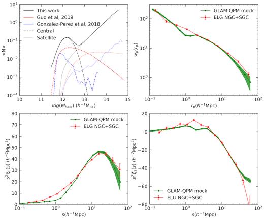
HOD model and galaxy clustering comparison between the GLAM-QPM mocks and ELG data. The upper left panel shows the best-fitting HOD model for the eBOSS ELG sample (black), where the dashed curve indicates the central HOD, dotted curve the satellite HOD, and the solid curve is the total HOD. The satellite fraction of our HOD model is |$17.4{{\ \rm per\ cent}}$|. As a comparison, we also show the HOD prediction for eBOSS ELG in the redshift range 0.8 < z < 0.9 from Gonzalez-Perez et al. (2018) (blue) and Guo et al. (2019) (red). The remaining three panels show the measurements of wp(rp), ξ0(s), and ξ2(s), respectively. The red curves are measurements from ELG data, averaged between the SGC and NGC, weighted by area. The errorbars are estimated using the jackknife resampling technique, with 25 jackknife samples. The green curves are the mean of the clustering of 100 GLAM-QPM mocks using the best-fitting HOD parameters in Table 2. The errorbars are the standard deviation, indicating the 1σ scatter.
Instead, we test the impact of HOD parameters to the small-scale clustering of ELGs by changing one parameter around the best-fitting parameter set. As shown in Fig. 7, we fix fmax = 0.15, σlog M = 0.25 and perturb other parameters around our fiducial parameter set in Table 2. The red curve shows the fiducial HOD parameter set, the blue and green curves show the clustering after the perturbation. Mmin and M1 affect the clustering of ELGs the most. This is because Mmin is the mean halo mass of the Gaussian function for central galaxies, so this parameter determines the halo mass scale that central galaxies reside in, and determines the ELG linear bias. M1 affects the mass of haloes that satellite galaxies reside in, so a smaller M1 would result in satellite ELGs being placed in higher mass haloes, increasing the linear bias. There is no significant change in the clustering even if we increase Mmin and M1 by a factor of 2. The impact of Mcut and α is even less. We conclude that by choosing suitable HOD parameters, we can produce mock catalogues with small-scale clustering that is in reasonable agreement with the data, and the large-scale bias is relatively insensitive to the parameters chosen.
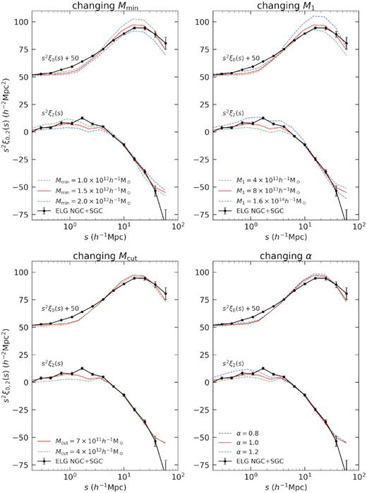
The impact of varying the fiducial HOD parameters on the redshift-space monopoles and quadrupoles. Redshift-space monopoles are vertically shifted by 50 to conveniently visualize. Our results for the fiducial set of HOD parameters (see Table 2) are shown with red curves, and each panel shows the result of perturbing one parameter at a time. The upper left panel shows the impact of varying Mmin, and the upper right panel shows the impact of varying M1. The lower panels show the impact of varying Mcut and α on the ELG clustering. The measured clustering of the eBOSS ELGs is indicated by the black points.
5 LARGE-SCALE CLUSTERING AND COVARIANCE MATRIX
5.1 Large-scale clustering
We generate 2000 galaxy mocks with the HOD parameters presented in Table 2, and cut the mock to the ELG chunk geometry as well as redshift distribution n(z). We measure the redshift-space monopole and quadrupole up to |$200 \,h^{-1}\,\rm {Mpc}$| using the same method and systematic weights as described in Section 3. We choose 40 equally spaced bins for s from 0 to 200 h−1 Mpc.
The large-scale clustering of the mocks is shown in Fig. 8, in comparison with the data. The shaded area indicates the 1σ and 2σ scatter in the 2000 mocks. The BAO feature can be clearly seen in the mocks, but there is some visible discrepancy between the mocks and data at the BAO scale, and also between the SGC and NGC. We first present the covariance matrix in Section 5.2, then test the statistical significance of the differences between SGC and NGC in Section 5.3.
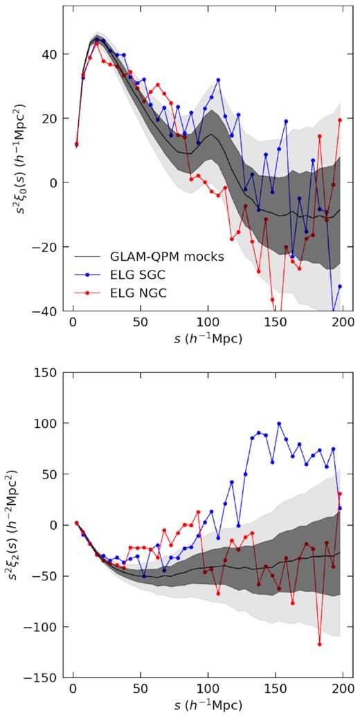
Large-scale clustering of ELG data and mocks. The upper panel shows redshift-space monopoles and lower panel shows redshift-space quadrupoles. The ELG SGC and NGC clustering are coloured in blue and red, respectively. The clustering of GLAM-QPM mock is shown in black, with the grey region showing the 1σ and 2σ range.
In Fig. 9, we compare the monopole and quadrupole of the ELG correlation function yielded by our GLAM-QPM mocks to that produced by the set of 1000 EZMocks of Zhao et al. (2020). The shape and amplitude of the clustering signals between the two mock sets are similar, despite the fact that they are achieved in very complementary ways. Whereas in the QPM method, ersatz halo populations are created and then populated with HOD models, in the EZMock approach the matter density field is mapped directly on to the galaxy density field, without haloes. The EZMocks further incorporate the effects of redshift evolution within the ELG sample, as well as some systematic errors accrued in target selection through the imaging data. These effects yield slightly higher sample variance estimates in the clustering, as seen in Fig. 9.
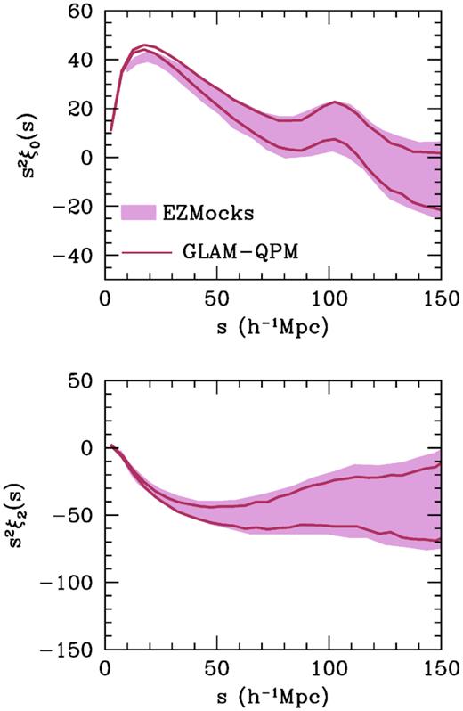
Comparison of the large-scale clustering between the GLAM-QPM mocks and EZMocks of Zhao et al. (2020). The upper panel shows the monopole and the lower panel shows the quadrupole. For both mocks, the lines and shaded regions indicate the 1σ errors on each quantity.
5.2 Covariance matrix
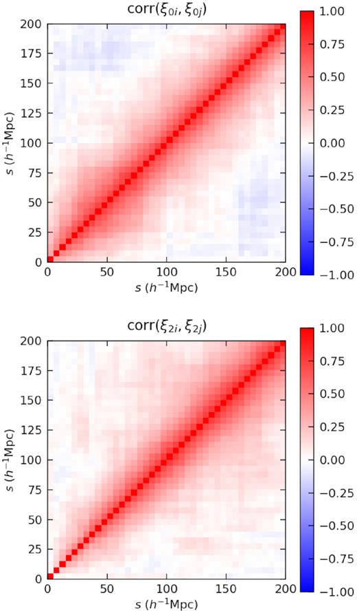
Correlation matrix of the GLAM-QPM mocks. The upper panel shows the correlation matrix of the monopole and the lower panel shows correlation matrix of the quadrupole. We use 40 equally spaced bins in s from 0 to 200 h−1 Mpc.
In Fig. 11, we show the correlation matrix for the ELG redshift-space monopole measurements at small scales. The result is as expected, with a correlation between galaxy pairs on scales |$s\gtrsim 2.5\,h^{-1}\,\rm Mpc$|, where the pairs are from two distinct haloes. Monopole measurements are uncorrelated on scales |$s\lesssim 2.5\, h^{-1}\,\rm Mpc$|, where galaxy pairs are within the same halo and galaxies are randomly sampled from the halo density profile.
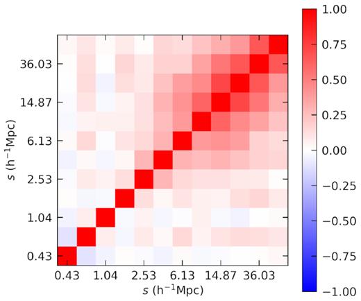
Correlation matrix for the ELG redshift-space monopole measurements at small scales. Distance separations are binned logarithmically from 0.34 to |$70\,h^{-1}\,\rm Mpc$|.
5.3 NGC and SGC difference
We use the GLAM-QPM mocks produced in this paper to test the consistency of the NGC and SGC measurements. For the redshift-space monopole at small scales, we measure the cross-|$\chi ^2=(\xi _{0_{\rm SGC}} - \xi _{0_{\rm NGC}})^TC_{\rm tot}^{-1}(\xi _{0_{\rm SGC}} - \xi _{0_{\rm NGC}})$| with 12 data points between 0.34 and 70 h−1 Mpc, where the covariance matrix Ctot = CNGC + CSGC is estimated using the GLAM-QPM mocks. We measure χ2/d.o.f. = 22.3/12 and conclude that on small scales, the SGC and NGC clustering measurements are compatible.
In order to see whether the difference between SGC and NGC at large scales is significant, we compute the cross-χ2 for both the monopole and the quadrupole measurements. We choose 10 linear s bins from |$77.5$| to |$122.5\,h^{-1}\rm Mpc$|, since we are most interested in the BAO scale at |$s\sim 100\,h^{-1}\rm Mpc$|. In Fig. 12,the results are χ2/d.o.f. = 12.53/10 for monopoles and χ2/d.o.f. = 14.91/10 for quadrupoles. The corresponding p-value is 0.25 and 0.14, meaning that the difference is insignificant and we cannot reject the null hypothesis that the difference between the SGC and NGC is caused by cosmic variance. We also build the χ2 distribution from our mock sample by selecting 200 NGC mocks and 200 SGC mocks (all from different GLAM simulations) and building the sample distribution from 40 000 χ2 values from each SGC–NGC pair. Our sample distribution agrees with the χ2 distribution with d.o.f. = 10 perfectly well, indicating that our covariance matrix are valid for robust BAO and RSD analysis, as is done in de Mattia (2020).
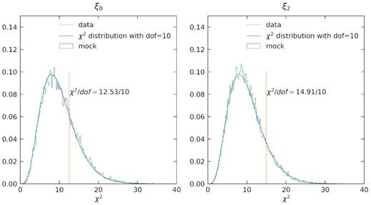
Cross-χ2 value from the SGC and NGC clustering measurements (vertical line), calculated using the covariance matrix from the GLAM-QPM mocks, given by |$\chi ^2= (\xi _{\rm SGC} - \xi _{\rm NGC})^TC_{\rm tot}^{-1}(\xi _{\rm SGC} - \xi _{\rm NGC})$|. The left-hand panel shows the χ2 for the monopole and the right-hand panel is for the quadrupole. We choose 10 r bins from 77.5 to |$122.5\,h^{-1}\,\rm Mpc$| to study the clustering signal around BAO peak |$(r\sim 100\,h^{-1}\,\rm Mpc)$|. We also show the χ2 distribution from 40 000 pairs of NGC and SGC mocks (blue histogram), in order to see where the data falls in the distribution. A χ2 distribution with d.o.f. = 10 is shown by the green curve.
6 SUMMARY
We present 2000 GLAM-QPM mock catalogues for the eBOSS DR16 ELG sample. We use GLAM simulations to produce the dark matter density field and the QPM method to assign dark matter haloes to particles in the simulation. The haloes are then populated with ELGs using an HOD methodology. We have calibrated the HOD parameters for the eBOSS ELG sample to model the large-scale bias of ELGs. The majority of central galaxies falls in haloes with mass between 1011 and |$10^{13}\,h^{-1}\,\rm M_\odot$|, and the satellite fraction of our HOD model is |$17.4{{\ \rm per\ cent}}$|. The eBOSS ELG survey geometry and radial selection functions are applied to our mocks. This set of mock catalogues is used in the eBOSS ELG RSD analysis in de Mattia (2020).
We have shown that the GLAM-QPM mock catalogues agree with ELG data at large scales, in general, within 2σ for monopole. For quadrupole the ELG SGC data shows higher clustering signal than GLAM-QPM mocks. We examined the cross-χ2 value for SGC and NGC around BAO scales, and find χ2/d.o.f. = 10.09/10 for the monopole and χ2/d.o.f. = 14.86/10 for the quadrupole. We cannot conclude that the difference between SGC and NGC are due to reasons other than cosmic variance.
ACKNOWLEDGEMENTS
SL is grateful to the support from CCPP, New York University. JLT and MRB are supported by NSF Award 1615997. FP and AK acknowledge support from the Spanish Ministry of Science and Innovation (MICINU) grant GC2018-101931-B-100. GR acknowledges support from the National Research Foundation of Korea (NRF) through grants nos. 2017R1E1A1A01077508 and 2020R1A2C1005655 funded by the Korean Ministry of Education, Science and Technology (MoEST), and from the faculty research fund of Sejong University. The GLAM simulations used in this paper were done on MareNostrum-4 at the Barcelona Supercomputer Center in Spain.
Funding for the Sloan Digital Sky Survey IV has been provided by the Alfred P. Sloan Foundation, the U.S. Department of Energy Office of Science, and the Participating Institutions. SDSS-IV acknowledges support and resources from the Center for High-Performance Computing at the University of Utah. The SDSS web site is www.sdss.org.
SDSS-IV is managed by the Astrophysical Research Consortium for the Participating Institutions of the SDSS Collaboration including the Brazilian Participation Group, the Carnegie Institution for Science, Carnegie Mellon University, the Chilean Participation Group, the French Participation Group, Harvard-Smithsonian Center for Astrophysics, Instituto de Astrofísica de Canarias, The Johns Hopkins University, Kavli Institute for the Physics and Mathematics of the Universe (IPMU)/University of Tokyo, Lawrence Berkeley National Laboratory, Leibniz Institut für Astrophysik Potsdam (AIP), Max-Planck-Institut für Astronomie (MPIA Heidelberg), Max-Planck-Institut für Astrophysik (MPA Garching), Max-Planck-Institut für Extraterrestrische Physik (MPE), National Astronomical Observatory of China, New Mexico State University, New York University, University of Notre Dame, Observatário Nacional/MCTI, The Ohio State University, Pennsylvania State University, Shanghai Astronomical Observatory, United Kingdom Participation Group, Universidad Nacional Autónoma de México, University of Arizona, University of Colorado Boulder, University of Oxford, University of Portsmouth, University of Utah, University of Virginia, University of Washington, University of Wisconsin, Vanderbilt University, and Yale University.
DATA AVAILABILITY
The GLAM-QPM mock galaxy catalogues will be published along with eBOSS DR16 galaxy catalogue release, and will also be placed at the Skies and Universes site (Klypin, Prada & Comparat 2017).1
