The MOSDEF survey: an improved Voronoi binning technique on spatially resolved stellar populations at z ∼ 2 Free

ABSTRACT

1 INTRODUCTION

Quantifying the distributions of stars, gas, and dust is an important step in understanding the formation and evolution of galaxies. For example, the locations of massive stars and their rates of formation can help address the assembly history of galaxies (e.g. Wuyts et al. 2012; Hemmati et al. 2014; Boada et al. 2015), the rate and efficiency with which gas is converted into stars (e.g. Lang et al. 2014; Jung et al. 2017; Tacchella et al. 2018), and a galaxy’s merger history (e.g. Conselice 2003; Lotz, Primack & Madau 2004; Lotz et al. 2008; Cibinel et al. 2015). Studying the structure of galaxies at z ∼ 2 is particularly relevant as cosmic star formation reaches its peak at this epoch, and galaxies were rapidly assembling their stellar mass (see Madau & Dickinson 2014).

Galactic structure can be assessed either qualitatively by eye (e.g. Hubble’s Tuning Fork; Hubble 1926) or quantitatively using parametric (e.g. Sérsic profile; Sérsic 1963) and non-parametric (e.g. CAS, Gini, M₂₀; Abraham, van den Bergh & Nair 2003; Conselice 2003; Lotz et al. 2004) metrics that measure the distribution of light. However, morphological classification schemes can potentially break down at higher redshifts. Compared to typical local galaxies, high-redshift galaxies are at an earlier stage in their evolution and appear clumpier and irregular in shape (e.g. Griffiths et al. 1994; Dickinson 2000; Papovich et al. 2005; Shapley 2011; Conselice 2014). Furthermore, since galaxies at z ∼ 2 are in the process of building the bulk of their stellar mass (Madau & Dickinson 2014), they are typically physically smaller in size due to their lower stellar masses (e.g. Toft et al. 2007; Trujillo et al. 2007; van der Wel et al. 2014; Scott et al. 2017; van de Sande et al. 2018) compared to their low-redshift counterparts. Observationally, these distant galaxies are also subject to the effects of cosmological dimming (see Barden, Jahnke & Häußler 2008), and the highest spatial resolution achievable with space-based facilities like the Hubble Space Telescope (HST) covers physically larger regions (few-kpc per resolution element) compared to that of lower redshift galaxies that are observed with the same instruments (sub-kpc per resolution element). Consequently, careful analyses are required when quantifying the morphology of galaxies (i.e. the distribution of stars, gas, and dust within galaxies) across a range of redshifts in an effort to infer how the structure of galaxies changes with cosmic time.

Several studies have explored resolved stellar populations in z ≳ 2 galaxies by fitting the observed pixel-to-pixel spectral energy distribution (SED) with stellar population synthesis models (Guo et al. 2012, 2015, 2018; Boada et al. 2015; Jung et al. 2017; Tacchella et al. 2018). While the highest resolution (for a given pixel scale) is obtained by fitting for the resolved SEDs within individual pixels, the signal to noise (S/N) within individual pixels may be too low such that the derived resolved stellar population properties may be unreliable. Furthermore, the signal may be correlated between adjacent pixels, given that the spatial resolution of the instrument (i.e. the point-spread function, or PSF) is larger than the size of the individual pixels. To compensate for these effects, several studies have implemented an adaptive Voronoi binning technique (Cappellari & Copin 2003) that groups pixels based on their S/N distribution such that low S/N pixels are grouped together into larger bins (e.g. Wuyts et al. 2012, 2013, 2014; Genzel et al. 2013; Lang et al. 2014; Tadaki et al. 2014; Chan et al. 2016). Typically, Voronoi bins are constructed using the S/N in a single filter, namely the H₁₆₀ band. However, for redder galaxies, such construction can lead to Voronoi bins with low S/N in bluer bands, resulting in poor constrains on the resolved stellar populations. If the S/N is not sufficiently high in at least five resolved filters (see Torrey et al. 2015), then the resulting best-fitting SEDs may not produce reliable stellar population inferred quantities for these bins.

In this work, we introduce an improved Voronoi binning method that groups pixels based on reaching a desired S/N threshold in multiple resolved filters. Our method improves the reliability of the derived stellar population parameters – albeit by sacrificing some spatial resolution – compared to the traditional single-filter approach for constructing Voronoi bins. In this paper, we apply our methodology to a sample of 350 star-forming galaxies drawn from the MOSFIRE Deep Evolution Field survey (MOSDEF; Kriek et al. 2015). The MOSDEF survey obtained rest-frame optical spectra for ∼1500 star-forming galaxies and active galactic nuclei (AGNs) at 1.4 ≲ z ≲ 3.8 that were drawn from the Cosmic Assembly Near-IR Deep Extragalactic Legacy Survey (CANDELS; Grogin et al. 2011; Koekemoer et al. 2011) and overlap with observations from the 3D-HST survey (Brammer et al. 2012; Skelton et al. 2014). Our study of the resolved stellar populations in high-redshift galaxies improves upon previous work. Previous resolved studies of z ≳ 2 galaxies either lacked accurate spectroscopic redshifts necessary to mitigate degeneracies in SED fitting (typically only photometric redshifts were used) or had samples with fewer than 100 galaxies (Wuyts et al. 2012; Guo et al. 2012, 2015, 2018; Tadaki et al. 2014; Boada et al. 2015; Jung et al. 2017; Tacchella et al. 2018). The statistically large sample of galaxies with robust spectroscopic redshifts and emission line measurements in the MOSDEF data set, on the other hand, enables an unprecedented view into the resolved stellar populations of z ∼ 2 galaxies. In this paper, we focus on the methodology of our Voronoi binning technique and demonstrate its utility. Detailed analysis of the resolved stellar population parameters obtained based on the new methodology will be presented in a follow-up paper.

The data, sample selection, and integrated stellar population synthesis modelling are presented in Section 2. In Section 3, our modified multifilter Voronoi binning technique for building stellar population and reddening maps is outlined. The resolved SEDs and SED-derived properties are compared to unresolved global quantities derived from the 3D-HST photometry in Section 4 and our modified multifilter Voronoi binning method is compared to the traditional single-filter Voronoi binning technique. Finally, the key points are summarized and we provide recommendations for resolved SED fitting analyses in Section 5.

All line wavelength measurements are given in vacuum and magnitudes are expressed in the AB system (Oke & Gunn 1983) throughout this paper. A cosmology with H₀ = 70 km s⁻¹ Mpc⁻¹, Ω_Λ = 0.7, and Ω_m = 0.3 is assumed.

2 DATA, SAMPLE SELECTION, AND INTEGRATED SED-DERIVED PROPERTIES

In this section, we present our observations, sample selection, and stellar population parameters inferred from fitting unresolved (integrated, or global) photometry. In Section 2.1, we discuss the high-resolution, multiwavelength CANDELS/3D-HST photometry from which we construct the resolved stellar population and reddening maps. The MOSDEF survey is described in Section 2.2, including the spectroscopic redshift measurements. The sample drawn from the parent MOSDEF survey is discussed in Section 2.3. Finally, in Section 2.4, we list the assumptions used to obtain global and resolved stellar population parameters.

2.1 CANDELS/3D-HST photometry

We use multiwavelength broad-band photometry from 0.3 to 8.0 μm in the five CANDELS (Grogin et al. 2011; Koekemoer et al. 2011) extragalactic fields: AEGIS, COSMOS, GOODS-N, GOODS-S, and UDS. CANDELS HST imaging covers ∼900 arcmin² and is 90 per cent complete at H₁₆₀ ∼ 25 mag. We make use of the publicly available¹ imaging and photometric catalogues that were processed and compiled by the 3D-HST grism survey team (Brammer et al. 2012; Skelton et al. 2014; Momcheva et al. 2016). The HST images were drizzled to a 0|${_{.}^{\prime\prime}}$|06 pixel⁻¹ scale and PSF convolved to the same 0|${_{.}^{\prime\prime}}$|18 spatial resolution as the H₁₆₀ data.

2.2 MOSDEF spectroscopy

Targets for the MOSDEF survey were selected from the five CANDELS extragalactic fields using the 3D-HST photometric and spectroscopic catalogues in three redshift bins (1.37 < z < 1.70, 2.09 < z < 2.61, and 2.95 < z < 3.80) such that the following strong rest-frame optical emission lines fall in near-IR windows of atmospheric transmission: [O ii]λ3727, 3730, H β, [O iii]λλ4960, 5008, H α, [N ii]λλ6550, 6585, and [S ii]λ6718, 6733. The targets were selected to an H₁₆₀-band limit of 24.0, 24.5, and 25.0 mag for the z = 1.37−1.70, 2.09−2.61, and 2.95−3.80 redshift bins (hereafter referred to as the z ∼ 1.5, z ∼ 2.3, and z ∼ 3 samples), respectively, corresponding to a stellar mass limit of ∼10⁹ M_⊙ for all three redshift bins. The galaxy identifications used throughout this paper refer to the 3D-HST v4 photometric catalogue.

The 4.5-yr MOSDEF survey obtained rest-frame optical spectra for ∼1500 star-forming and AGN galaxies using the MOSFIRE multiobject spectrograph (McLean et al. 2010, 2012) in the Y, J, H, and K bands (R = 3400, 3000, 3650, and 3600 using 0|${_{.}^{\prime\prime}}$|7 slit widths) on the 10-m Keck I telescope. Every slit mask also included at least one slit star, which is used for the absolute flux calibration and corrections for slit loss. Line fluxes are measured by fitting a linear function to the continuum and a Gaussian function to each emission line. For the [O ii]λλ3727, 3730 doublet and Hα+[N ii]λλ6550, 6585 lines, a double and triple Gaussian is fit the the lines, respectively. The stellar population model that best fits the observed 3D-HST photometry (Section 2.4) is used to correct H α and H β line fluxes for underlying Balmer absorption. Flux errors are obtained from the 68th-percentile width of the distribution of line fluxes that have been remeasured from the 1D spectra that have been perturbed by their error spectra 1000 times. Finally, the spectroscopic redshift is measured from the observed wavelength of the highest S/N emission line, which is typically H α or [O iii]λ5008. Refer to Kriek et al. (2015) and Reddy et al. (2015) for additional details on the MOSDEF survey, including the observing strategy, data reduction, and line flux measurements.

In this study, the redshift of each galaxy (and its resolved components) is fixed to the measured MOSDEF spectroscopic redshift in order to constrain the stellar population parameters derived from the SED fitting.

2.3 Sample selection

Our sample is derived from the MOSDEF parent sample in the z ∼ 1.5 and z ∼ 2.3 redshift bins. First, only galaxies with robust spectroscopic redshifts that have been measured using at least two emission features with an S/N >2 are selected. AGNs are removed based on their identification through their X-ray luminosities, optical emission lines (log ([N ii]/H α) > −0.3), and/or mid-IR luminosities (Coil et al. 2015; Azadi et al. 2017, 2018; Leung et al. 2019). This initial sample contains 830 star-forming galaxies at 1.24 < z < 2.66, including 74 galaxies that were serendipitously detected outside of the targeted MOSDEF redshift bins. Additional constraints to the S/N and resolution of the photometry are applied when performing adaptive Voronoi binning (see Section 3.2), which brings our sample to 350 star-forming galaxies at redshifts 1.25 < z < 2.66.

The spectroscopic redshift distribution, SFR–M_* relation, and size–M_* relation are shown in Fig. 1 for the galaxies in our initial (white histogram; empty circles) and final (grey histogram; filled circles) samples. Also shown is the median SFR, size, and stellar mass of our sample divided into four equally sized bins (yellow stars). The SFR bins are, on average, 0.16 dex above the main sequence relation defined in Shivaei et al. (2015), which is within the intrinsic scatter of the relation. Our final selected sample is marginally biased against low-mass and low-SFR galaxies, primarily due to the tendency of such galaxies to be compact and/or faint. It is difficult to spatially resolve compact galaxies into several components and faint galaxies do not have sufficient S/N for measuring reliable spatially resolved fluxes across several filters. Therefore, these factors cause low-mass and low-SFR galaxies to be excluded from our sample during the Voronoi binning procedure (see Section 3.2).

Figure 1.

Left: Spectroscopic redshift distribution of galaxies in our sample covering two redshift bins: 1.24 < z < 1.74 and 1.84 < z < 2.66. The white histogram shows the initial sample distribution (830 galaxies). The grey histogram denotes our primary sample (350 galaxies) that results after S/N restrictions are applied in the Voronoi binning procedure (see Section 3.2). Middle: H α SFR versus stellar mass, i.e. the star-forming main sequence. H α emission is corrected for dust using the Balmer decrement and assuming the Cardelli, Clayton & Mathis (1989) extinction curve. All H α SFRs are calculated assuming a Chabrier (2003) IMF and 20 per cent Solar metallicity (see Section 2.4). The solid green line (extended by the dashed line for visual clarity) is the best linear fit to the SFR–M_* relation based on the first 2 yr of data from the MOSDEF survey (Shivaei et al. 2015). The empty and filled circles show the galaxies in the initial (830) and final samples (350), respectively. The yellow stars are the medians of the individual points of the 350 galaxies in our sample, equally divided into four bins of stellar mass. Right: The size–M_* relation for our initial and selected samples, with the same symbol colouring as the middle panel. The area is measured from the detected 3D-HST segmentation map region for each galaxy. Our final sample selection is marginally biased against compact, low-mass galaxies due to the S/N requirements imposed by the Voronoi binning procedure (see Section 3.2).

Open in new tabDownload slide

2.4 Spatially unresolved SED fitting

The stellar populations are modelled on both resolved (see Section 3.4) and unresolved scales for galaxies in our sample to obtain SED-derived E(B − V)_stars, stellar population ages, SFRs, and stellar masses. Here, we describe the SED fits to the integrated galaxy light, as measured from the 3D-HST photometric catalogues. A χ² minimization technique is used to select the Bruzual & Charlot (2003) stellar population model that best fits the observed photometry (see Reddy et al. 2012). First, the photometry is corrected for the strongest emission lines measured in the MOSDEF spectroscopy, including H α, H β, [O iii]λλ4960, 5008, and the [O ii]λ3728 doublet. In the SED modelling, we assume a Chabrier (2003) initial mass function (IMF), constant star-formation histories (SFHs), and allow the ages to range between 50 Myr and the age of the Universe at the redshift of each galaxy.² Reddening in the range |$0.0 \le {E(B-V)_{\rm {stars}}}\ \le 0.4$| is considered while assuming a Small Magellanic Cloud (SMC) extinction curve (Fitzpatrick & Massa 1990; Gordon et al. 2003) and sub-solar metallicity (0.2 Z_⊙).³

Typical SED parameter errors are derived using a subset of 50 randomly selected galaxies from our sample that span the SED fitting parameter space in E(B − V)_stars, stellar population age, SFR, and stellar mass in both redshift bins. Only 50 galaxies are selected for the error analysis in the interest of limiting computation time, but the range of SED parameters probed by these 50 galaxies is similar to that of the larger sample. The measured fluxes are perturbed 100 times by their flux errors and refit. The width of the parameter space of the 68 (of 100) models with the lowest χ² relative to the observed photometry is assumed to represent the errors in the SED parameters. The typical SED parameter error is then estimated as the average of the errors from all galaxies in the subsample. The typical random SED parameter errors derived from the SEDs fit to the perturbed 3D-HST photometry are as follows: 0.01 in E(B − V)_stars, 0.20 dex in log stellar population age, 0.05 dex in log SFR, and 0.16 dex in log stellar mass.

3 RESOLVED STELLAR POPULATION AND REDDENING MAPS

3.1 Resolved photometry

The resolved stellar population and reddening maps are constructed using HST/WFC3 resolved imaging in the F125W, F140W, and F160W filters (hereafter J₁₂₅, JH₁₄₀, and H₁₆₀), and HST/ACS resolved imaging in the F435W, F606W, F775W, F814W, and F850LP filters (hereafter B₄₃₅, V₆₀₆, i₇₇₅, I₈₁₄, and z₈₅₀). Note that not all of the filters are available for all of the CANDELS fields. The resolved imaging is supplemented with unresolved Spitzer/IRAC photometry at 3.6 μm, 4.5 μm, 5.8 μm, and 8.0 μm, which has been corrected for contamination by neighbouring sources using models of the HST images that have been PSF-smoothed to the lower resolution IRAC photometry. Pixels associated with the 3D-HST photometry are identified using the Source Extractor (Bertin & Arnouts 1996) segmentation maps provided by the 3D-HST grism survey (Skelton et al. 2014), which are based on a noise-equalized combination of J₁₂₅+JH₁₄₀+H₁₆₀.

3.2 Adaptive Voronoi binning

Construction of the resolved stellar population and reddening maps begins with isolating individual galaxies in our sample. Sub-images that are 80 × 80 pixels in size (4|${_{.}^{\prime\prime}}$|8 × 4|${_{.}^{\prime\prime}}$|8, or approximately 40 × 40 kpc at z ∼ 2) are cut for each galaxy from the CANDELS/3D-HST imaging and its respective spatially matched noise map. The 3D-HST segmentation map is then used to mask any pixels not associated with the galaxy. The median of the pixels that are unassociated with any detected sources is used to apply a local background subtraction to each pixel of the sub-image, although the correction is negligible since the CANDELS images are already background subtracted.

The modifications applied to the Cappellari & Copin (2003) algorithm add constraints only while building the Voronoi bins. Unmodified processes include the pixel selection while building candidate bins, the ‘roundness’ threshold of a candidate bin, or the assignment of unsuccessfully binned pixels after the bins have been created. We refer the reader to Cappellari & Copin (2003) for further details on their adaptive Voronoi binning technique. Here, we describe how Voronoi bins are constructed, given our modifications (refer to Fig. 2 for a visual outline). The layout of the Voronoi bins is based on the S/N distribution of a primary filter (H₁₆₀ is used, similar to other studies), although the S/N distribution in all applicable filters is considered. A candidate bin begins with the unbinned pixel that has the highest S/N in the primary filter and then neighbouring pixels are added to the bin until the specified target S/N is reached in all applicable filters. The modified algorithm also includes designating an optional minimum Voronoi bin size. The smallest Voroni bins are constrained to contain at least 3 pixels (in contrast with typical Voronoi binning schemes that allow single pixels to be Voronoi bins) such that they match the HST PSF resolution of 0|${_{.}^{\prime\prime}}$|18, translating to the smallest resolution elements having an area of ∼0.75 kpc². If this binning procedure fails (for example, the entire galaxy has been grouped into a single bin), the process is repeated using one less filter – specifically, the filter with the lowest (S/N)_total as calculated in equation (2) (note that the primary filter is always required). Upon each failed binning attempt, this procedure will repeat iteratively until only the primary filter remains. If all other filters have been rejected, the revised adaptive Voronoi binning algorithm is applied to the primary filter (H₁₆₀) alone using an S/N that is twice that of the original target S/N (S/N = 10, matching the requirements used by previous studies). However, for this study, we require that the bins be defined by multiple filters that span the Balmer and 4000 Å breaks in order to more robustly quantify ages and stellar masses on a bin-by-bin basis. Therefore, any galaxies that failed to be adaptively binned using at least two filters (H₁₆₀ and one additional filter) are removed from our sample.

Figure 2.

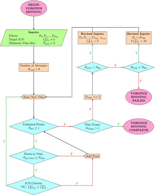
Flowchart highlighting the modifications we applied to the Cappellari & Copin (2003) adaptive Voronoi binning algorithm. For this study, the primary filter is F₀ = H₁₆₀, the target signal to noise is (S/N)_t = 5, and the minimum number of pixels per Voronoi bin is N_min = 3. N_filt is the number of additional filters used in addition to the primary filter, N_trial is the number of times adaptive Voronoi binning has been attempted, N_pix is the number of unbinned pixels remaining, N_pix,Vbin is the number of pixels within the Voroni bin being constructed, and N_Vbins is the total number of Voronoi bins after all pixels have been assigned into a Voronoi bin.

Open in new tabDownload slide

As an example, Fig. 3 shows how the S/N distribution for one of the galaxies in our sample (UDS 21834, z = 1.67) varies between the H₁₆₀ and V₆₀₆ filters on the pixel-to-pixel level in panels (a) and (b) and across the Voronoi bins in panels (d) and (e). Panel (f) in Fig. 3 shows the number of filters that have an S/N ≥ 5 in each Voronoi bin. For comparison, panel (c) shows the number of filters that have an S/N ≥ 5 on the pixel-to-pixel level. Torrey et al. (2015) found that applying a simplified set of SED fitting assumptions (i.e. dust-free, restricted ages, and limited metallicities) to a sample of simulated galaxies observed in five filters reproduced stellar masses within a factor of 2 of the known simulated mass. Therefore, reliable best-fitting SEDs are expected to be produced from the regions where an S/N ≥ 5 is reached in at least five filters, as is represented by the darkest blue colour in panels (c) and (f) of Fig. 3. By comparing the areas covered by the darkest blue colour in panels (c) and (f), it can be seen that a larger region of the galaxy can be used for reliable SED fitting when adaptive Voronoi binning is applied with a multifilter requirement. For this reason, we consider only Voronoi bins that have an S/N ≥ 5 in a minimum of five filters for the primary SED fitting. Throughout the text, we refer to the bins with an S/N ≥ 5 in at least five filters as the ‘Voronoi bins.’ We also ensure that the high S/N filters cover both sides of the Balmer and 4000 Å break region, which further constrains the stellar population age estimates. Bins that are not above the target S/N contain the ‘remaining’ signal and tend to be in the outskirts of the galaxy [light blue bins shown in panel (f) of Fig. 3]. The bins that have less than five filters with S/N ≥ 5 are referred to as ‘outskirt’ components of the galaxy. Collectively, the high S/N Voronoi bins combined with the outskirt bins cover exactly the same area defined by the 3D-HST segmentation map. In Section 4, the integrated SED and its respective parameters derived from the conservatively selected Voronoi bins are compared to those derived from additionally including the outskirt components. It is specifically noted when outskirt bins are included in the analysis, but outskirt bins are typically not included as their SED-derived properties are more uncertain due to the lower S/N in these bins.

Figure 3.

The S/N maps before and after applying adaptive Voronoi binning for one of the galaxies in our sample, UDS 21834 (z = 1.67). Only the 911 pixels and 41 bins identified by the segmentation map are shown. Top row: the pixel-to-pixel S/N distribution in (a) H₁₆₀ and (b) V₆₀₆. Panel (c) shows that for each pixel, the number of filters (N_filt) have an S/N ≥ 5. Bottom row: the Voronoi bin S/N distribution in the (d) H₁₆₀ and (e) V₆₀₆ filters. Panel (f) shows that for each Voronoi bin, the number of filters have an S/N ≥ 5. The Voronoi bins within the darkest blue region match our criteria of an S/N ≥ 5 in ≥5 filters, which throughout the text will be referred to simply as the ‘Voronoi bins.’ All other lighter blue regions make up the ‘outskirt’ component and will be referred to as such throughout the text.

Open in new tabDownload slide

Galaxies that have less than five Voronoi bins (outskirt bins do not contribute) remaining are removed from our sample, as they are considered unresolved. Galaxies in our sample have 5–151 Voronoi bins (∼16 bins on average), as is shown by the histogram in Fig. 4. On average, an individual Voronoi bin contains ∼18 pixels (∼4.5 kpc²) and the median bin size is 6 pixels (1.5 kpc²). Overall, the Voronoi binning procedure reduces the sample size from the 830 star-forming galaxies discussed in Section 2.3 to 350 galaxies. As can be seen in Fig. 1, the Voronoi binning requirements marginally biases our sample against low-mass, low-SFR, and compact galaxies.

Figure 4.

Distribution of the number of Voronoi bins within each galaxy in our sample. To be included in our sample, galaxies must have at least five Voronoi bins. The black dashed vertical line shows the average number of Voronoi bins per galaxy, N = 16. The median Voronoi bin size is 6 pixels and the minimum Voronoi bin size is set to 3 pixels.

Open in new tabDownload slide

3.3 Flux measurements

The counts in the convolved science images and noise maps are converted to flux density, and the AB magnitude and magnitude error are calculated within each Voronoi bin. The minimum magnitude error is set to 0.05 mag, in order to prevent any single photometric point from skewing the SED fit.

Using the normalization defined by equation (3) forces the H₁₆₀–IRAC colours to be constant across the entire galaxy, thus constraining the strength of the Balmer and 4000 Å breaks for the highest redshift galaxies in our sample (z ≳ 2.5). As the Balmer/4000 Å break is sensitive to stellar population age and attenuation (e.g. Worthey 1994; Shapley et al. 2001), we must be wary of how fixing the H₁₆₀–IRAC colour affects the derived age and reddening maps. In Appendix  B, we investigate how variations in the H₁₆₀–IRAC colours influence the distribution of stellar population ages and reddening inferred through the SED fitting. In general, we find that the redder Voronoi bins remain red [higher E(B − V)_stars] and the bluer Voronoi bins remain blue [lower E(B − V)_stars] when their H₁₆₀–IRAC colours are perturbed, indicating that our constraint on the H₁₆₀–IRAC colours (i.e. equation 3) does not unduly influence the results concerning the distribution of stellar population ages and attenuation within galaxies.

3.4 Resolved SED fitting

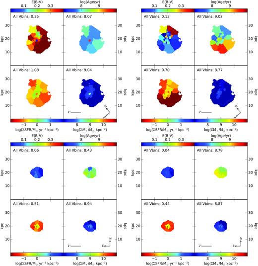
The same model assumptions that were outlined in Section 2.4 are also used for the resolved SED fitting. For each galaxy in our sample, two representations of the integrated properties are obtained by fitting a single SED to (a) the multiwavelength 3D-HST broad-band photometry (Skelton et al. 2014, see Section 2.4) and (b) the total sum of the flux within all of the valid Voronoi bins (including the total 3D-HST IRAC fluxes). Resolved SED modelling is performed on all of the individual Voronoi bins and outskirt components. In Section 4, we compare the resolved and integrated SED fitting results and demonstrate how using only the high S/N Voronoi bins does not significantly affect the results from the SED fitting (see Section 3.2). Fig. 5 shows the resolved stellar population and reddening maps for UDS 21834 (z = 1.67) and COSMOS 3666 (z = 2.09) as examples. The average E(B − V)_stars, average stellar population age, summed SFR, and summed stellar mass derived from the Voronoi bins are listed in the top left corner of each panel in Fig. 5.

Figure 5.

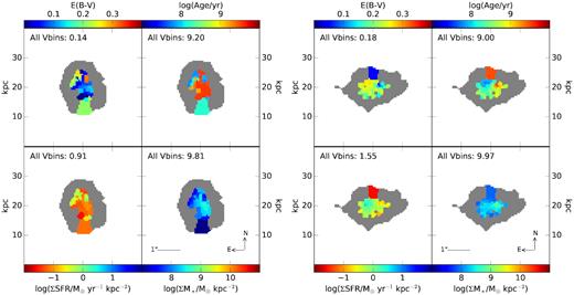
Stellar population and reddening maps from resolved SED fitting for UDS 21834 (z = 1.67, left-hand panels) and COSMOS 3666 (z = 2.09, right-hand panels), showing the distribution of E(B − V)_stars (top left), stellar population age (top right), SFR (bottom left), and stellar mass (bottom right). These galaxies both have 41 Voronoi bins with the bins containing an average of 8 and 6 pixels (∼2 kpc² and ∼1.5 kpc²), respectively. The grey regions indicate the outskirt component consisting of regions that are included in the segmentation map but do not fulfill the Voronoi bin criteria (S/N ≥ 5 in at least five filters) discussed in Section 3.2. The listed number in each panel shows the average E(B − V)_stars or stellar population age weighted by the Voronoi bin areas or the summed SFR or stellar mass from all of the Voronoi bins.

Open in new tabDownload slide

Typical resolved SED parameter errors are derived using the same subset of 50 galaxies as was used to obtain the integrated SED parameter errors (see Section 2.4). Only 50 galaxies are selected for the error analysis in the interest of limiting computation time, but the range of SED parameters probed by these 50 galaxies is similar to that of the larger sample. The measured fluxes in each Voronoi bin are perturbed 100 times by their flux errors and refit. The width of the distribution of parameters for the 68 (of 100) models with the lowest χ² relative to the observed photometry is assumed to represent the errors in those parameters for each individual Voronoi bin. Within a single galaxy, the SED parameter errors of the individual Voronoi bins are averaged together, resulting in a typical Voronoi bin error within the individual galaxy. Finally, the typical Voronoi bin SED parameter error is estimated as the average of the typical Voronoi bin errors from all 50 galaxies in the subsample. The typical SED parameter errors derived from the SEDs fit to the perturbed Voronoi bin fluxes are as follows: 0.03 in E(B − V)_stars, 0.21 dex in log stellar population age, 0.16 dex in log SFR, and 0.10 dex in log stellar mass.

4 RESOLVED VERSUS INTEGRATED PROPERTIES

In comparing the resolved and integrated stellar population parameters, we must be aware of the different apertures over which the measurements are made and the slightly different methodology used to fit the SEDs. Specifically, the integrated 3D-HST flux measurements are based on the flux within 0|${_{.}^{\prime\prime}}$|7 apertures and are corrected for the contribution from the strongest emission lines that were detected in the MOSFIRE spectra, including [O ii]λ3727, 3730, H β, [O iii]λλ4960, 5008, and H α (Reddy et al. 2015). The resolved Voronoi bin fluxes, on the other hand, are measured directly from the sum of the flux detected by the pixels in the resolved imaging and are not corrected for the contribution of the emission lines detected by MOSDEF. Additionally, the integrated 3D-HST photometry covers a larger dynamic range in wavelength than the range covered by the filters that are available for resolved photometry due to the ancillary ground-based data that are available. While the Spitzer/IRAC photometry is included to increase wavelength coverage of the resolved photometry, we assume that the H₁₆₀–IRAC colours are fixed across all resolved elements using equation (3). Despite these inherent differences between the integrated and resolved photometry, the V₆₀₆ − H₁₆₀ colours measured from the integrated 3D-HST fluxes and the sum of the flux from all Voronoi bins and outskirt components agree within the measured scatter of 0.3 mag.

The biases that may arise from differences between the resolved and unresolved photometry are explored by directly comparing the associated best-fitting SEDs (Section 4.1) and SED-derived parameters (Section 4.2). In Section 4.3, we show how our modified multifilter Voronoi binning technique can improve upon that using the H₁₆₀ filter alone by comparing the best-fitting SEDs and SED-derived parameters from the two techniques. Finally, the implications of our findings on resolved stellar population studies are discussed in Section 4.4.

4.1 Comparing best-fitting SEDs

The unresolved and summed resolved SEDs for eight galaxies in our sample that span the SED fitting parameter space (low/high E(B − V)_stars, stellar population age, SFR, and stellar mass) are shown in Fig. 6. The summed best-fitting SEDs derived from the resolved Voronoi bin photometry (light blue points and curves) are compared to the SEDs derived from the unresolved photometry (black points and curves). The 3D-HST photometry (black points) has extended wavelength coverage and includes more light than the valid Voronoi bins (light blue points) – typically 0.85 mag brighter. The summed Voronoi bin SEDs do not include ‘outskirt’ components, which are defined as low S/N regions in Section 3.2. Therefore, Fig. 6 additionally shows the SEDs that result from adding the outskirt component SEDs to the summed Voronoi bin SEDs (red points and curves). The total flux from the sum of the Voronoi bins and outskirt components is nearly equivalent to the measured flux from the unresolved 3D-HST photometry for filters with resolved imaging (red and black points). Similarly, the summed resolved SEDs that include outskirt components are nearly identical to the unresolved SEDs obtained from the 3D-HST photometry (red and black curves).⁴ Note that not all galaxies, such as GOODS-N 21507, have an outskirt component as all of the regions have sufficient S/N to be included as Voronoi bins.

Figure 6.

Best-fitting SEDs for eight example galaxies spanning the SED fitting parameter space. From top to bottom, each row, respectively, shows example galaxies with low (left) and high (right) E(B − V)_stars, stellar population ages, SFRs, and stellar masses. The black points are the fluxes from the 3D-HST photometric catalogue (Skelton et al. 2014) corrected for the brightest MOSDEF emission lines and the black curves are their respective best-fitting SEDs. The light blue points are the total integrated fluxes within the Voronoi bins (Voronoi bins with S/N ≥ 5 in at least five different filters). The light blue curves represent the sum of the SEDs that are best fit to the individual Voronoi bins. The red points indicate the total flux obtained when summing the Voronoi bin and outskirt bin fluxes, which naturally lie close to the values obtained from the 3D-HST photometry. The red curves show the SED fits to the red points. Photometric errors are typically smaller than the size of the points. Note that not all galaxies have outskirt components, such as GOODS-N 21507.

Open in new tabDownload slide

From Fig. 6, we conclude that the shapes of the SEDs are generally well preserved between the resolved and integrated results (with the exception of galaxies similar to AEGIS 8907, which are further discussed in Section 4.2). The primary difference between the resolved and integrated SEDs is the normalization, which is attributed to the fact that the Voronoi bins contain less light than the broad-band measurements. This causes the Voronoi bins to exhibit systematically lower stellar masses and SFRs compared to the 3D-HST photometry (as expected), but, on average, the offset is less than the uncertainties in the SED-derived stellar masses and SFRs.

4.2 Comparison of SED-derived parameters

The shapes of the resolved SEDs are generally consistent with the unresolved SEDs presented (Fig. 6), but several galaxies exhibit summed resolved SEDs that are systematically offset from the integrated SED. The E(B − V)_stars and stellar population age derived from the SED that is best fit to the integrated 3D-HST photometry are compared to the average E(B − V)_stars and stellar population age derived from the Voronoi bins weighted by the area of each Voronoi bin.⁵ The stellar masses and SFRs derived from the SED fit to the integrated photometry are compared to the sum of the stellar mass and SFR within all of the Voronoi bins. While the SED normalization differences caused by different area coverage between the Voronoi bins and the integrated photometry do cause systematically lower stellar masses and SFRs, we find that, on average, all SED-derived parameters inferred from the resolved SEDs are within 1 standard deviation of those derived from the integrated 3D-HST photometry.

A notable exception is that the resolved SEDs of the z ∼ 1.5 galaxies are, on average, redder and younger than indicated by the broad-band SED fits, as is showcased by AEGIS 8907 in Fig. 6. The AEGIS 8907 photometry demonstrates that this discrepancy is caused by the lack of resolved imaging covering the rest-frame UV for our z ∼ 1.5 sample. The number of filters that cover the UV slope depends on the field, where all of the z ∼ 1.5 galaxies in AEGIS, COSMOS, or UDS have only one HST filter available that covers the UV slope (1250–2500 Å). We find that the best-fitting SEDs prefer redder and younger solutions when the UV slope is unconstrained. Only above redshifts z ≳ 2.1 do AEGIS, COSMOS, and UDS galaxies have at least two filters covering the UV slope. The left-hand panel of Fig. 7 demonstrates how the resolved SED fitting of the z ∼ 1.5 sample produces redder inferred E(B − V)_stars compared to those from the unresolved broad-band SED fits, while the preference for redder E(B − V)_stars completely disappears for the z ∼ 2.3 sample. Similarly, the right-hand panel of Fig. 7 shows how the redder E(B − V)_stars and younger stellar ages in the z ∼ 1.5 sample cause the derived SFRs from the Voronoi plus outskirt bins⁶ to be overestimated compared to SFRs inferred from the 3D-HST photometry. The discrepancy between the inferred E(B − V)_stars derived from the unresolved and resolved photometry in the z ∼ 1.5 sample occurs at all E(B − V)_stars values that are probed by the SED model grid [|$0.0\le {E(B-V)_{\rm {stars}}}\le 0.4$|] and does not correlate with stellar mass, such that the measured differences in E(B − V)_stars are not likely associated with our choice in dust attenuation curve (see footnote 3). However, there may be intrinsic differences in the stellar populations between the two redshift samples.

Figure 7.

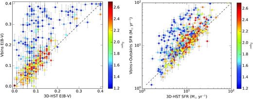
Left: The average Voronoi bin E(B − V)_stars weighted by the area of the Voronoi bins versus the E(B − V)_stars derived from the 3D-HST photometry. Right: The total SFR of the Voronoi plus outskirt bins versus the SFR derived from the 3D-HST photometry. The points are colour-coded by their spectroscopic redshift. The dashed black line indicates where the E(B − V)_stars or SFR derived from the Voronoi bins equals those inferred from the 3D-HST photometry. Only the galaxies in the z ∼ 1.5 sample exhibit E(B − V)_stars or SFRs that deviate significantly from those derived from the 3D-HST photometry due to the lack of resolved imaging covering the UV slope (e.g. AEGIS 8907 in Fig. 6).

Open in new tabDownload slide

In order to further investigate whether the redder inferred E(B − V)_stars are caused by the lack of UV slope coverage or differences between the intrinsic stellar populations in the two redshift bins, we select 111 galaxies from our z ∼ 2.3 sample that have observations in at least seven resolved HST filters. The two bluest filters observed are removed such that only one remaining filter covers the UV slope, with at least five resolved filters remaining for the SED fitting. As can be seen in the right-hand panel of Fig. 7, when the resolved SED fitting (see Section 3.4) is repeated, we find that the average E(B − V)_stars inferred across all Voronoi bins are redder than that inferred when there are additional filters covering the UV slope. Therefore, we conclude that the inferred E(B − V)_stars values for the z ∼ 1.5 sample are overestimated due to there being fewer than two filters covering the UV slope. Fig. 8 shows how the sum of the resolved SEDs changes (thick light blue curve compared to the thick purple curve) when the two bluest filters covering the UV slope are removed (red crosses) for GOODS-N 22669 (z = 2.13). For context, a subset of the SED models are also shown, where each colour represents a step in E(B − V)_stars for a range of stellar population ages (i.e. the black, blue, green, yellow, and red SEDs represent SED models with |$0\le {E(B-V)_{\rm {stars}}}\le 0.4$| in steps of 0.1 mag, respectively). There are three significant features that can be seen in Fig. 8: (1) when the UV photometry is included, the shape of the best-fitting SED is primarily constrained by the rest-frame UV photometry (light blue curve); (2) when the UV photometry is not included, the shape of the best-fitting SED is primarily constrained by the rest-frame optical photometry (purple curve); and (3) the SED fits generally under-predict the IRAC photometry. The IRAC photometry may be brighter than what can be fit with the model SEDs in the rest-frame near-IR due to the higher sensitivity and larger aperture over which these measurements are made. Systematically brighter IRAC fluxes and the known discrepancy between stellar population age and extinction in the SED models at optical wavelengths (e.g. Worthey 1994; Shapley et al. 2001) may together explain why there is a bias towards redder best-fitting SEDs when the UV slope is unconstrained (such as AEGIS 8907).

Figure 8.

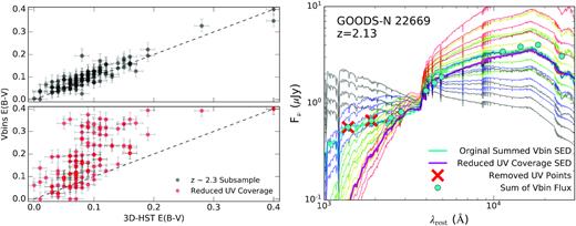
Left: The average Voronoi bin E(B − V)_stars weighted by the area of the Voronoi bins versus the E(B − V)_stars derived from the 3D-HST photometry for the z ∼ 2.3 galaxies. The black points show the original E(B − V)_stars of the z ∼ 2.3 galaxies (top). The red points show how removing the two bluest filters from the z ∼ 2.3 galaxies reproduces the relative reddening observed in the z ∼ 1.5 sample (bottom). Right: The sum of the model SEDs that best fit the resolved Voronoi bins for GOODS-N 22669 (z = 2.13). The thick light blue curve shows the summed SED that includes all of the data from the resolved imaging (blue points). The thick purple curve shows the summed SED where the data from the two bluest filters were not included in the SED fitting (red crosses). The faded curves in black, blue, green, yellow, and red represent SED models with E(B − V)_stars equal to 0.0, 0.1, 0.2, 0.3, and 0.4, respectively. Several curves of the same colour are shown to demonstrate how the SED model shape varies with different stellar population ages when E(B − V)_stars are held constant.

Open in new tabDownload slide

The lack of UV slope coverage in the resolved Voronoi bin fitting for the z ∼ 1.5 sample may complicate inferences of the intrinsic variation in the reddening distribution for these galaxies. However, rather than observing a flat reddening distribution in the z ∼ 1.5 galaxies, structure is observed in the E(B − V)_stars maps (e.g. see Fig. 5 for UDS 21834 at z = 1.67) due to the reddening and ages being constrained in part by the strength of the Balmer/4000 Å breaks in the SED fitting. Finally, we note that the SED-derived SFRs and stellar masses are constrained by the overall normalization of the SED, and they are minimally affected by the lack of observations covering the UV slope.

4.3 Traditional Voronoi binning

In constructing the Voronoi bins in Section 3.2, we enforce more stringent requirements (minimum 3 pixels and S/N ≥ 5 in five filters) than the ‘traditional’ Voronoi binning procedure (S/N ≥ 10 in H₁₆₀) performed in previous studies (Wuyts et al. 2012, 2013, 2014; Genzel et al. 2013; Lang et al. 2014; Tadaki et al. 2014). In this section, the results from our multifilter Voronoi binning technique are directly compared to the traditional Voronoi binning approach using the same subset of 50 galaxies that were used to determine the typical SED errors (see Sections 2.4 and 3.4). Only 50 galaxies are selected for this analysis in the interest of limiting computation time, but the range of SED parameters probed by these 50 galaxies is similar to that of the larger sample. The traditional Voronoi bins are constructed using the original Cappellari & Copin (2003) algorithm (version 3.0.4), which exclusively requires each Voronoi bin to attain an S/N ≥ 10 in the H₁₆₀ filter alone. Traditional Voronoi bin construction failed for one galaxy, resulting in a final subsample of 49 galaxies for this exercise.

The left-hand panel of Fig. 9 shows that the average E(B − V)_stars inferred across the traditional Voronoi bins determined by the H₁₆₀-band alone are typically redder (higher) compared to the average E(B − V)_stars inferred from the multifilter determined by Voronoi bins. For context, the average E(B − V)_stars derived from both Voronoi binning procedures are also compared to the E(B − V)_stars derived from the unresolved 3D-HST photometry in the right-hand panel of Fig. 9. We find that the average E(B − V)_stars inferred from the traditional H₁₆₀-only Voronoi bins (red points and stars) are, on average, 0.02 mag redder (higher) than our multifilter approach (light blue points and stars) in both redshift bins but deviate as much as 0.20 mag. Meanwhile, the E(B − V)_stars from our multifilter approach are 0.10 and 0.02 mag redder (higher) than the 3D-HST globally derived E(B − V)_stars (black dashed line) for our z ∼ 1.5 and z ∼ 2.3 samples, respectively. For the z ∼ 1.5 sample, the likely explanation as to why both resolved methods exhibit redder (higher) E(B − V)_stars compared those derived from the unresolved 3D-HST photometry is that the UV slope is unconstrained by the available resolved data, as explained in Section 4.2. Meanwhile, the differences between the E(B − V)_stars derived from our multifilter technique and the unresolved 3D-HST photometry are, on average, smaller than the differences in the E(B − V)_stars derived from the traditional Voronoi binning technique and the unresolved 3D-HST photometry. This is due to the larger Voronoi bin sizes inherent to our technique that are consequently less resolved compared to Voronoi bins that are defined by a single filter.

Figure 9.

Left: The average E(B − V)_stars weighted by the area of the Voronoi bins derived from the ‘traditional’ Voronoi bins derived from the H₁₆₀ S/N distribution exclusively versus the Voronoi bin distribution derived from several filters (see Section 3.2). The Spearman rank correlation coefficient and its significance are listed in the top left corner. Right: The average E(B − V)_stars weighted by the area of the Voronoi bins derived from both Voronoi binning schemes compared to the E(B − V)_stars inferred from the 3D-HST photometry for both redshift samples. The red points represent the ‘traditional’ Voronoi binning technique and the light blue points represent our multifilter Voronoi binning technique. The red and light blue stars are the averages from individual points equally divided into four bins of E(B − V)_stars in the x-axis. The black dashed lines indicate where the E(B − V)_stars derived from all sources are equal.

Open in new tabDownload slide

The differences observed between the E(B − V)_stars inferred from the H₁₆₀-derived Voronoi bins and the multifilter-derived Voronoi bins could also be explained by the high S/N requirement for bluer filters in the multifilter technique, in that it will force blue regions of the galaxy to be included with intrinsically red regions. Forcing additional blue light to be included with intrinsically red regions would cause the multifilter Voronoi bins to typically exhibit systematically shallower UV slopes compared to traditionally defined Voronoi bins – particularly those covering the reddest regions of the galaxy. Therefore, in Fig. 10, the resolved SEDs that cover the same spatial areas from the two methodologies are directly compared such that they have the same total fluxes (light blue and red points). Individual Voronoi bins built from the multifilter procedure (Section 3.2) are typically larger than traditionally constructed Voronoi bins based only on the H₁₆₀ filter. Specifically, Fig. 10 shows examples of the resolved SEDs from the traditional Voronoi bins (black points and grey curves) that entirely make up an individual Voronoi bin from the multifilter procedure (light blue points and curves). As can be seen, there are examples where the shape of the summed SEDs derived from the traditionally defined H₁₆₀-only Voronoi bins (light blue curves) either matches (left column) or deviates (right column) from the shape of the SEDs derived from the multifilter Voronoi bins covering the same region (red curves). Based on the matching UV slopes from the examples shown in the left column of Fig. 10 and the fact that the discrepant SED examples in the right column have been compared over the same resolved regions where all filters contain the same total flux, we conclude that bluer light being forced into the multifilter Voronoi bins does not serve as an adequate explanation to the observed systematic difference between the E(B − V)_stars inferred from the two methodologies in Fig. 9. However, Fig. 10 also shows that the best-fitting SEDs from the multifilter technique are typically more tightly constrained by the higher S/N photometry than the SEDs fit to the smaller Voronoi bins constructed from the H₁₆₀ filter alone. The inclusion of any resolved components with low S/N at short wavelengths appears to cause the summed best-fitting SEDs to exhibit steeper UV slopes that result in redder (higher) E(B − V)_stars for galaxies in both the z ∼ 1.5 and z ∼ 2.3 samples (right column of Fig. 10). Furthermore, since the discrepancy between the UV slopes of the two Voronoi binning methods is observed in both of our redshift bins, it is important to note that the redder inferred E(B − V)_stars from the summed traditional SEDs are independent from the redder E(B − V)_stars that are caused by the lack of resolved UV slope coverage in the z ∼ 1.5 sample (see Section 4.2). Overall, the preference towards redder SEDs tends to occur when the UV slope is generally poorly constrained (in this case by large photometric errors or, as discussed in Section 4.2, limited data).

Figure 10.

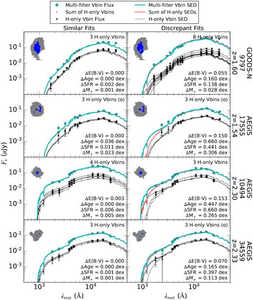
Examples of the best-fitting SEDs from the Voronoi bins built from the H₁₆₀ filter alone compared to best-fitting SED of the single Voronoi bin constructed from our multifilter procedure (Section 3.2) that covers the same physical area as the H₁₆₀-only Voronoi bins. The black points represent the fluxes within the H₁₆₀-only Voronoi bins, which add up to the fluxes from a single, larger Voronoi bin built using our new criteria (light blue/red points). The errors for the light blue/red points are typically smaller than the size of the points. The grey curves are the SEDs that are best fit to the H₁₆₀-only Voronoi bin fluxes. The red curves represent the sum of the grey curves and are generally hidden behind the light blue curves that represent the SEDs that are best fit to the individual Voronoi bin constructed from our multifilter procedure. The number of H₁₆₀-only Voronoi bins is listed in the top right corner of each panel and an (o) is shown if the matched multifilter Voronoi bin is considered an outskirt component. The values in the bottom right corner of each panel show the differences in E(B − V)_stars, stellar population age, SFR, and stellar mass inferred from the integrated H₁₆₀-only Voronoi bin SEDs versus the individual Voronoi bin from our multifilter procedure. The image in the top left corner of each panel shows for each galaxy: the segmentation map area in grey, the area where the Voronoi bins have an S/N ≥ 5 in at least five filters in dark blue, and the individual Voronoi bin that is represented by the curves in light blue. The two columns show examples where the summed SEDs (light blue and red curves) are similar (left column) or discrepant (right column) compared to each other.

Open in new tabDownload slide

Based on the results presented here, we find that traditionally defined Voronoi bins result in resolved SEDs that are systematically redder [higher E(B − V)_stars] than multifilter defined Voronoi bins. This systematic effect is due to the lower S/N in bluer filters when constructing Voronoi bins based only on the distribution of H₁₆₀-band light. By extension, we expect SED fitting across individual pixels to exhibit redder (higher) E(B − V)_stars as well. In order to best constrain the shape of the SEDs that are fit to resolved photometry, we recommend using a binning procedure that enforces high S/N across both blue and red resolved filters – especially covering the UV slope and Balmer/4000 Å breaks. Additionally, caution should be taken when including regions that have low S/N overall (i.e. ‘outskirt’ components) in resolved studies.

4.4 Discussion

The structure of high-redshift galaxies can give insight into the evolution of galaxies on resolved scales (see Conselice 2014). In particular, the SFR of a galaxy is an important measure of how galaxies build their stellar mass. However, the intrinsic SFR of a galaxy must be inferred by correcting for the obscuring effects of dust. The scattering and attenuation of starlight by dust depend on the amount and distribution of dust (e.g. Draine & Lee 1984; Fitzpatrick & Massa 1986; Calzetti, Kinney & Storchi-Bergmann 1994; Calzetti et al. 2000), which is typically accounted for by assuming an attenuation curve. Obtaining accurate dust reddening on resolved scales may inform the assumptions made when fitting unresolved photometry, such as the slope and shape of the dust attenuation curve (Reddy et al. 2018; Shivaei et al. 2020). While stellar masses are generally quite robust to methodology, we have shown throughout this paper that the inferred resolved reddening can be difficult to constrain due to a combination of the age–extinction–metallicity degeneracy (Worthey 1994; Shapley et al. 2001; see Appendix  B), unconstrained UV slopes (see Section 4.2), and generally low S/N resolved rest-frame UV photometry (see Section 4.3). In such cases, Voronoi bins constructed based on multiple filters may be desirable in order to obtain more robust resolved stellar population parameters and, in particular, robust reddening maps.

In Appendix  B, we discussed how constraining the Balmer/4000 Å breaks is important for breaking the age-extinction degeneracy (Worthey 1994; Shapley et al. 2001), particularly for galaxies at z > 2.5 where the Balmer/4000 Å breaks shift into the H₁₆₀ filter. Through our choice of normalizing the unresolved IRAC photometry by the resolved H₁₆₀ flux, we made the assumption that the resolved H₁₆₀–IRAC colours are constant across all bins in each galaxy. We showed that constraining the H₁₆₀–IRAC colours does not significantly influence the distribution of stellar population ages and reddening within galaxies. While only 15 galaxies in our sample are at z > 2.5, constraining the Balmer/4000 Å breaks by assuming a constant H₁₆₀–IRAC colour distribution may be a viable solution for resolved studies at higher redshifts.

Throughout this paper, we showed that if the UV slope is not well constrained by the resolved photometry, such as at lower redshifts (z < 2.1; see Section 4.2) or by low S/N regions (see Section 4.3), then the derived resolved stellar populations properties may be biased towards SEDs with redder (higher) E(B − V)_stars. If the inferred E(B − V)_stars are overestimated, then observed SFRs may consequently be overcorrected for dust attenuation, which would result in the inferred intrinsic SFRs also being overestimated (see Fig. 7). This observational reddening bias most significantly affects our z ∼ 1.5 sample, where only one resolved filter covers the UV slope (see Section 4.2), but more generally, this systematic bias has a greater influence on intrinsically blue galaxies (young, dust-free stellar populations) opposed to intrinsically red galaxies (old, dusty stellar populations). A Wuyts et al. (2012) methodology can be implemented to adjust the resolved SEDs to better reproduce the integrated SED shape in cases where it is not possible to obtain at least two resolved filters covering the UV slope (1250–2500 Å) but at the cost of increased uncertainty in the specific distribution of the resolved stellar population properties (see Appendix  A). For galaxies where the resolved UV slope is not well constrained due to low S/N, we introduced a technique in Section 3.2 that increases the S/N across all resolved filters to produce more reliable SEDs that are fit to the resolved photometry at the cost of a marginally decreased resolution compared to previous methods (see Section 4.3). Our multifilter Voronoi binning technique increases the number of resolved elements that can confidently recover resolved stellar population parameters through SED fitting, particularly for galaxies with low surface brightness or extended diffuse light.

Based on the analyses presented throughout this paper, we provide a list of recommendations for confidently deriving resolved stellar population properties. (1) If possible, ensure that at least two photometric observations span key rest-frame SED features, particularly the UV slope and Balmer/4000 Å breaks. (2) Incorporate a binning technique that either includes information about the S/N distribution of both red and blue filters or otherwise ensures that at least five filters are significantly detected – especially shorter wavelength filters that are typically lower S/N. (3) Generally be wary of biases that may exist between resolved properties that are inferred from well- (e.g. full wavelength coverage, S/N ≥ 5 in five filters) versus poorly constrained (e.g. unconstrained SED features, ‘outskirt’ components) SEDs.

5 SUMMARY

In this paper, we presented an improved Voronoi binning technique for studying resolved stellar populations at high redshifts, which overall aims to increase the confidence in the best-fitting SEDs and stellar population properties that are derived from the resolved photometry. The layout of the resolved components for performing resolved SED fitting was determined from the S/N distribution of multiple filters in the high-resolution CANDELS/3D-HST imaging for a sample of 350 star-forming galaxies drawn from the MOSDEF survey at spectroscopic redshifts 1.25 < z < 2.66. The stellar population and dust maps were constructed based on our new multifilter Voronoi binning technique and their integrated stellar population properties were compared to those derived from the unresolved broad-band imaging and those derived from a ‘traditional’ Voronoi binning approach that used the H₁₆₀ filter alone to determine Voronoi bins. Our main conclusions are summarized as follows.

• In Section 3.2, we described a modified Voronoi binning technique (see Fig. 2) that accounts for the S/N distribution of multiple resolved filters opposed to the H₁₆₀ filter alone. In order for an individual Voronoi bin to be included in our analysis, we required the bin to contain an S/N ≥ 5 in at least five resolved filters. Any bins that did not satisfy this criteria were deemed ‘outskirt’ components (see Fig. 3).

• We found that the shapes of the summed resolved SEDs from our multifilter binning technique were generally consistent with the SEDs that were fit to the unresolved broad-band photometry (see Fig. 6) in Section 4.1. Similarly, in Section 4.2, we found that the average E(B − V)_stars, average stellar population ages, summed SFRs, and summed stellar masses are typically within 1 σ of the stellar population properties derived from the unresolved broad-band photometry.

• The most significant deviation between the resolved and unresolved SEDs and best-fitting stellar population parameters was the shape of the UV slope and the average E(B − V)_stars inferred from the resolved reddening maps for galaxies in the z ∼ 1.5 sample (see Fig. 7). By removing rest-frame UV photometry from the z ∼ 2.3 sample and repeating the resolved SED fitting, we determined in Section 4.2 that the discrepancy in the z ∼ 1.5 inferred reddening is most likely caused by the lack of data that are able to constrain the UV slope (1250–2500 Å).

• When comparing our multifilter Voronoi binning technique (S/N ≥ 5 in at least five filters) with a ‘traditional’ single-filter approach (S/N ≥ 10 in H₁₆₀) in Section 4.3, we found that the single-filter technique results in E(B − V)_stars values that are systematically redder by 0.02 mag, on average, than our multifilter method but could deviate by as much as 0.20 mag (see Fig. 9). We also found that our multifilter technique produces average inferred E(B − V)_stars that are closer to those derived from the unresolved broad-band photometry compared to the single-filter approach, but we note that this may be expected from the larger (i.e. lower resolution) bins that are inherent to our technique. We also demonstrated through Fig. 10 that systematically redder UV slopes may result from poorly constrained rest-frame UV photometry, which can occur in the smaller, traditionally defined Voronoi bins. Finally, we note that SED-derived stellar masses remain robust between methodologies when all Voronoi bins are included.

The methodology presented here will be applied to future resolved analyses using the MOSDEF data set, which will additionally incorporate results from the rest-frame optical emission line measurements. In general, we advocate for a methodology that best constrains the SEDs that are best fit to the resolved photometry. Well-constrained SEDs can generally be obtained by using high S/N multiband photometry that covers key features in the rest-frame SED (i.e. UV slope, Balmer/4000 Å breaks). Furthermore, low S/N ‘outskirt’ regions could be excluded from analyses; otherwise, biases between well- and poorly constrained resolved SEDs must be understood when interpreting the results. Finally, we note that higher confidence in resolved stellar population parameters through the methods presented here comes at the cost of lower resolution. However, these methods will similarly push to higher resolutions when applied to future high-resolution imaging instruments, such as the NIRcam on the upcoming James Webb Space Telescope.

ACKNOWLEDGEMENTS

This work is based on observations taken by the CANDELS Multi-Cycle Treasury Program and the 3D-HST Treasury Program (GO 12177 and 12328) with the NASA/ESA HST, which is operated by the Association of Universities for Research in Astronomy, Inc., under NASA contract NAS5-26555. The MOSDEF team acknowledges support from an NSF AAG collaborative grant (AST-1312780, 1312547, 1312764, and 1313171) and grant AR-13907 from the Space Telescope Science Institute, grant NNX16AF54G from the NASA ADAP program, and Chandra archival award AR6-17011X. Some of the data presented herein were obtained at the W.M. Keck Observatory, which is operated as a scientific partnership among the California Institute of Technology, the University of California, and the National Aeronautics and Space Administration. The Observatory was made possible by the generous financial support of the W.M. Keck Foundation. The authors wish to recognize and acknowledge the very significant cultural role and reverence that the summit of Maunakea has always had within the indigenous Hawaiian community. We are most fortunate to have the opportunity to conduct observations from this mountain.

Facilities: HST (WFC3, ACS), Keck:I (MOSFIRE), Spitzer (IRAC)

Software:astropy (Astropy Collaboration 2013, 2018), matplotlib (Hunter 2007), numpy (Oliphant 2007), scipy (Oliphant 2007), and Voronoi Binning Method (Cappellari & Copin 2003).

DATA AVAILABILITY

Resolved CANDELS/3D-HST photometry is available at: https://3dhst.research.yale.edu/Data.php (Grogin et al. 2011; Koekemoer et al. 2011; Brammer et al. 2012; Skelton et al. 2014; Momcheva et al. 2016). Spectroscopic redshifts from the MOSDEF survey are available at: http://mosdef.astro.berkeley.edu/for-scientists/data-releases/ (Kriek et al. 2015).

Footnotes

REFERENCES

APPENDIX A: THE WUYTS ET AL. (2012) METHOD

In order to best constrain stellar mass estimates determined from the resolved SED fitting and constrain the shape of the resolved SEDs in the near-IR, we elect to include the unresolved Spitzer/IRAC photometry with the resolved photometry. Wuyts et al. (2012) presented a method for incorporating unresolved photometry into the results of resolved SED fitting by modifying the best-fitting resolved SEDs such that their sum produces an SED that is optimally fit to the integrated photometry. We alternatively use a simple normalization based on the H₁₆₀ flux to directly use the IRAC photometry in the resolved SED fitting (see Section 3.3 and equation 3). In this appendix, we compare the best-fitting SEDs and SED-derived properties that result from the simple normalization we assumed versus the Wuyts et al. methodology. For this investigation, we select GOODS-N 21507 (z = 1.57), AEGIS 8907 (z = 1.59), COSMOS 6750 (z = 2.13), and GOODS-N 17714 (z = 2.23), thus including two galaxies from our z ∼ 1.5 and z ∼ 2.3 redshift bins.

In Fig. A1, we show the sum of the resolved SEDs from both our method (red curves) and the Wuyts et al. method (dark blue curves) compared to the SED that is fit to the unresolved 3D-HST photometry (black curves and points). The contribution from outskirt bins is included to best compare the summed SEDs with the SED that is fit to the unresolved 3D-HST photometry, but we note that a small normalization offset remains in some cases due to minor differences in the apertures (see the beginning of Section 4).⁷ With the exception of AEGIS 8907, the integrated SEDs are consistent with each other. As discussed in Section 4.2, the UV slope of AEGIS 8907 is not well constrained due to there being only one resolved filter available at 1250–2500 Å. Therefore, our SED fitting procedure prioritizes fitting the data in the near-IR that is covered by the IRAC photometry, whereas the Wuyts et al. method emphasizes the shape of the optical photometry initially and later adjusts to best match the integrated 3D-HST SED.

Figure A1.

Best-fitting integrated SEDs from three different SED-fitting methods for four example galaxies. The colours of the points and curves are the same as in Fig. 6. The black points and curves show the fluxes from the 3D-HST photometry and the respective best-fitting SED. The red points and curves indicate the total flux from all Voronoi bins (including outskirts) and the sum of their best-fitting resolved SEDs for the IRAC data that have been normalized to the H₁₆₀ flux [see Section 3.3 and equation (3)]. The dark blue curves show the sum of the resolved SEDs that have alternatively been modified to include the IRAC photometry using the method described by Wuyts et al. (2012). The errors are typically smaller than the size of the points. Note that not all galaxies have outskirt components, such as GOODS-N 21507.

Open in new tabDownload slide

The resolved SEDs that are fit to the flux contained within each Voronoi bin are compared between our method and the Wuyts et al. method for AEGIS 8907 and GOODS-N 17714 in Fig. A2. We remind the reader that the SEDs from the Wuyts et al. method (dark blue curves) show the SEDs that have been adjusted to produce a better match to the integrated photometry, such that the stellar population model has changed and the individual resolved SEDs may not necessarily match the resolved UV and optical photometry. Fig. A2 shows that the resolved SEDs are most discrepant in outskirt bins (panels with red points and curves), whereas the resolved SEDs generally agree between the two methods for the well-constrained Voronoi bins (S/N ≥ 5 in at least five  filters; panels with light blue points and curves). It is important to note that because the resolved stellar population models have changed in the Wuyts et al. method, the distribution of resolved properties may not be well preserved – particularly in outskirt bins where the resolved SEDs are less constrained. However, in cases such as AEGIS 8907, the Wuyts et al. method better reproduces the overall shape of the integrated 3D-HST photometry since the UV slope is unconstrained by the resolved photometry for low-redshift objects using our methodology (see Section 4.2). In most cases though, the sum of all the resolved SEDs from both methods represents good fits to the unresolved photometry. Finally, the resolved stellar population and dust maps (including outskirts) are shown in Fig. A3 for AEGIS 8907 (top panels) and GOODS-N 17714 (bottom panels) from our method (left-hand panels) and the Wuyts et al. method (right-hand panels). We find that most cases are similar to GOODS-N 17714, where the resolved SED properties are comparable between the two methods. For cases like AEGIS 8907, the SFR and stellar mass distributions are also consistent between the two methods, with the greatest deviation being in the E(B − V)_stars distribution. As stated previously, the UV slope of AEGIS 8907 is not well constrained by the resolved photometry alone, such that the discrepancy in the resolved E(B − V)_stars distribution is unsurprising.

Figure A2.

The resolved SEDs for every Voronoi and outskirt bin comparing the two methods that incorporate the unresolved IRAC photometry for AEGIS 8907 (top panels) and GOODS-N 17714 (bottom panels). The colours of the points and curves are the same as in Fig. 6 and Fig. A1. The first panel is the same as in Fig. 6 but also includes the light blue points and curves that show the sum of the flux and SEDs from the well-constrained Voronoi bins (S/N ≥ 5 in at least five  filters). The panels with light blue points and curves show resolved SEDs fit to Voronoi bins and the panels with red points and curves show resolved SEDs fit to outskirt bins. The light blue and red SED curves directly include the IRAC photometry in the resolved SED fitting by normalizing the IRAC flux by the H₁₆₀ resolved flux (see equation 3). The dark blue curves show the resolved SEDs that have been modified to include the contribution of the IRAC photometry using the method described by Wuyts et al. (2012). Note that in some cases, particularly in the outskirt bins, there is no change between the original SED and the SED modified by the Wuyts et al. method, such that the SED curves overlap in the figure. The labels in each panel indicate the central pixel coordinate of each bin.

Open in new tabDownload slide

Figure A3.

Stellar population and reddening maps from the resolved SED fitting (including outskirt components) that incorporates IRAC photometry using a normalization based on the H₁₆₀ flux (left-hand panels) and the method described by Wuyts et al. (2012) (right-hand panels). The distribution of E(B − V)_stars (top left), stellar population age (top right), SFR (bottom left), and stellar mass (bottom right) is shown for AEGIS 8907 (z = 1.59, top panels) and GOODS-N 17714 (z = 2.23, bottom panels). The listed number in each panel shows the average E(B − V)_stars or stellar population age weighted by the Voronoi bin areas or the summed SFR or stellar mass from all of the Voronoi bins.

Open in new tabDownload slide

In this work, we are interested in best preserving the distribution of the resolved stellar populations. Therefore, we elect to directly include the IRAC photometry in the resolved SED fitting by normalizing the IRAC photometry by the H₁₆₀ flux contained in each resolved element (see equation 3). In this appendix, we have shown that the results obtained through the Wuyts et al. method are comparable to those obtained through our methodology. However, the Wuyts et al. method may be more appropriate in situations where key SED features (e.g. UV slope, Balmer/4000 Å breaks) cannot be constrained by the resolved photometry but at the cost of the specific distribution of stellar population properties being more uncertain. Throughout our analysis, we retain separation between our z ∼ 1.5 and z ∼ 2.3 samples due to the discrepancies in the inferred E(B − V)_stars caused by the UV slope being unconstrained by the resolved photometry.

APPENDIX B: H₁₆₀–IRAC COLOUR PERTURBATIONS

In Section 3.3, we normalized the unresolved Spitzer/IRAC photometry by the H₁₆₀ flux in each resolved element to accommodate for different area coverage. However, this unrealistically assumes that the IRAC flux directly traces the H₁₆₀-band flux. Most critically, this impacts galaxies at redshifts z ≳ 2.5, where the Balmer/4000 Å breaks shift into the H₁₆₀ filter and the break strength becomes constrained exclusively by the IRAC photometry. As a probe of stellar population age, the strength of the Balmer/4000 Å breaks is crucial towards breaking the age-extinction degeneracy (e.g. Worthey 1994; Shapley et al. 2001), where the shape of the SED in the rest-frame UV to near-IR of a young, dusty stellar population looks similar to an old, dust-free population. In this appendix, the H₁₆₀–IRAC colours are perturbed to simulate spatially resolved variations in the IRAC photometry to assess how constraining the H₁₆₀–IRAC colours influences the integrated and resolved stellar population properties, with special care towards the stellar population ages and reddening. For this investigation, we select GOODS-S 36093, GOODS-N 20924, COSMOS 6750, and UDS 22341, thus including two galaxies with redshifts above (2.62 and 2.55) and below (2.20 and 1.38) z = 2.5.

The H₁₆₀–IRAC colours are perturbed in all Voronoi bins simultaneously while maintaining a constant total flux. The H₁₆₀–IRAC colour shift is calculated for each resolved element based on a normal distribution centred on the average of the four H₁₆₀–IRAC colours (where the IRAC flux is calculated by equation 3) and a width of 1.0 mag. The proposed perturbations are restricted to be physically plausible values by requiring the H₁₆₀–IRAC perturbations to fall within the range of the H₁₆₀–IRAC colours in the Bruzual & Charlot (2003) stellar population synthesis model templates (constant SFH at the known redshift). The H₁₆₀–IRAC colours are perturbed for all but one Voronoi bin in the galaxy. If the sum of the perturbed IRAC fluxes is less than the original total IRAC flux, then the remaining Voronoi bin is attributed the leftover IRAC flux. Otherwise, if the sum of the perturbed IRAC fluxes add up to be greater than the original total IRAC flux, then all of the perturbations are repeated. The ‘leftover’ bin often appears as an outlier in our results, but it does not alter the conclusions made here. An individual galaxy is perturbed n times, where n is the number of Voronoi bins in the galaxy, such that for each iteration, a different Voronoi bin receives the leftover IRAC flux. In summary, for a given galaxy with n Voronoi bins, the entire resolved distribution is perturbed n times with every iteration having the same total flux. Finally, we use the perturbed IRAC fluxes to repeat the integrated and resolved SED modelling.

In Fig. B1, the SED-derived properties are compared between the original results with constant H₁₆₀–IRAC colours and the perturbed solutions. Regardless of redshift, we find that a perturbed Voronoi bin (black points) on average (green circles) has the same properties as the case of constant H₁₆₀–IRAC colours (x-axis values) and by extension maintains its intrinsic colour. Fig. B2 shows an example (GOODS-S 36093, z = 2.62) of how the resolved reddening and stellar population ages change with each perturbation of the H₁₆₀–IRAC colours, further demonstrating that the colours do not vary significantly from bin to bin. While the Voronoi bin that received the leftover IRAC flux is occasionally seen as an outlier, the average E(B − V)_stars or stellar population age (values in the bottom right corner of each panel in Fig. B2) remains consistent. In general, the average of the resolved distribution for all SED-derived properties is comparable with the average of the original distribution (light blue stars in Fig. B1). Therefore, we conclude that we are not unduly constraining the resolved stellar ages or reddening by simplifying the IRAC flux distribution through our use of equation (3).

Figure B1.

The SED-derived E(B − V)_stars, stellar population ages, SFRs, and stellar masses for each Voronoi bin as the H₁₆₀–IRAC colours are perturbed. Each row represents a single galaxy from our sample for a spread of redshifts. Each vertically connected green line represents a single Voronoi bin that has been perturbed n times, where n is the number of Voronoi bins in the galaxy. The black points along a single vertical line show how the SED-derived properties change as that single Voronoi bin is perturbed, compared to the original values. Each green circle is the average of the perturbed results within a single Voronoi bin, compared to the original value. The light blue stars compare the average of the Voronoi bins over n perturbations with the average of the original distribution (see Fig. B2). The errors of the blue stars show the spread in the averaged Voronoi bins over all n perturbations. The dashed black lines indicate where the perturbed properties equal the original properties.

Open in new tabDownload slide

Figure B2.

E(B − V)_stars (top) and stellar population age (bottom) maps for GOODS-S 36093 (z = 2.62). The top left-hand panels show the original E(B − V)_stars and stellar population age distribution from SED fitting, where the H₁₆₀–IRAC colours are constant across all Voronoi bins (see equation 3). All other panels show the E(B − V)_stars and stellar population age distributions when SED fitting was performed on the H₁₆₀–IRAC colour perturbations. The value in the bottom right of each panel is the average E(B − V)_stars or log stellar population age (in dex) derived from the entire galaxy area.

Open in new tabDownload slide

Author notes