


ABSTRACT
In a previous paper, we reported simulations of the evolution of the magnetic field in neutron star (NS) cores through ambipolar diffusion, taking the neutrons as a motionless uniform background. However, in real NSs, neutrons are free to move, and a strong composition gradient leads to stable stratification (stability against convective motions) both of which might impact on the time-scales of evolution. Here, we address these issues by providing the first long-term two-fluid simulations of the evolution of an axially symmetric magnetic field in a neutron star core composed of neutrons, protons, and electrons with density and composition gradients. Again, we find that the magnetic field evolves towards barotropic ‘Grad–Shafranov equillibria’, in which the magnetic force is balanced by the degeneracy pressure gradient and gravitational force of the charged particles. However, the evolution is found to be faster than in the case of motionless neutrons, as the movement of charged particles (which are coupled to the magnetic field, but are also limited by the collisional drag forces exerted by neutrons) is less constrained, since neutrons are now allowed to move. The possible impact of non-axisymmetric instabilities on these equilibria, as well as beta decays, proton superconductivity, and neutron superfluidity, are left for future work.
1 INTRODUCTION
Neutron stars (NSs) are classified in several types based on their substantially different observational properties, which appear to be determined mainly by their rotation rates, magnetic field strengths, and presence or absence of accretion from a binary companion. In particular, the magnetic fields control the torque that slows down their rotation, can have a crucial effect on the free energy budget and radiation processes, and influence the flow of accreted matter on and around these stars. On the other hand, the structure and evolution of these magnetic fields is far from understood as different classes of NSs have very different magnetic field strengths, which appear to be correlated with their age. Young NSs; such as magnetars, classical radio pulsars, and high-mass X-ray binaries; have strong surface magnetic fields ∼1011–15 G; while the much older low-mass X-ray binaries and millisecond pulsars have weaker fields ∼108–9 G (Kaspi 2010; Viganò et al. 2013). This suggests a magnetic field decay, which is usually attributed to the accretion process (Backer et al. 1982; Bhattacharya 1991, 1995; Tauris & van den Heuvel 2006), but might also be explainable through its own dynamics and spontaneous decay as the NS cools and ages (Cruces, Reisenegger & Tauris 2019). Furthermore, the high time-averaged luminosity of magnetars is thought to be linked to the decay of their magnetic field, since their rotational energy loss is insufficient to account for it. Since these objects appear to be isolated, their field decay must be attributed to processes intrinsic to the NSs (Thompson & Duncan 1995, 1996). Therefore, understanding the mechanisms that drive the long-term evolution of the magnetic field in NSs may help us unveil the relation between their different classes.
The physics of the evolution of the magnetic field varies in different regions of the NS (Goldreich & Reisenegger 1992). For example, in the solid crust, ions have very restricted mobility, so the currents are carried by electrons. Therefore the long-term mechanisms that control the evolution of the field in this region are Ohmic diffusion, i.e. current dissipation by electric resistivity; and Hall drift which corresponds to the transport of the magnetic flux by the electron motion. Since the magnetic field dynamics is intrinsically non-linear, its recent studies have mainly taken a numerical point of view (Hollerbach & Rüdiger 2002; Pons & Geppert 2007; Pons, Miralles & Geppert 2009; Viganò, Pons & Miralles 2012; Gourgouliatos et al. 2013; Viganò et al. 2013; Lander & Gourgouliatos 2019), finding that the magnetic field evolves towards stable ‘attractor’ configurations (Gourgouliatos & Cumming 2014; Marchant et al. 2014).
In this work, we concentrate on the long-term magnetic field dynamics in the core of NSs, which is conceptually much more involved than in the crust. Indeed, the core of an NS is a fluid mixture of neutrons, protons, and electrons, joined by other species at increasing densities. The mechanisms for field evolution in this region are strongly dependent on the star’s core temperature T. Shortly after the NS is formed, neutrons and charged particles are strongly coupled by collisions, behaving essentially as a single fluid, coupled to the magnetic flux. This fluid is stably stratified by its composition gradient (due to the different density profiles of charged particles and neutrons) (Pethick 1992; Goldreich & Reisenegger 1992; Reisenegger 2009); thus, strong buoyancy forces oppose convective motions. However, as noted by Reisenegger (2007), weak interaction processes (so-called ‘Urca reactions’; Gamow & Schoenberg 1941; Haensel 1995) can quickly adjust the composition of a fluid element, overcoming stable stratification and allowing the fluid to transport the magnetic flux. In this ‘strong-coupling’ regime, the matter can be regarded as a single, stably stratified, non-barotropic fluid (i.e. pressure depends on the non-uniform chemical composition in addition to density). However, as weak interactions are strongly temperature dependent, this regime applies only for a very short time after the NS birth (while T ≳ 5 × 10⁸ K). As the star cools, the progressive reduction of the collisional coupling makes relative motions possible, so the charged particles can carry the magnetic flux with a different velocity field than that of the neutrons, a process called ‘ambipolar diffusion’ (Pethick 1992; Goldreich & Reisenegger 1992). Hence, on long time-scales, the NS core is in a ‘weak-coupling’ regime, in which neutrons and charged particles act as independent barotropic fluids (assuming charged particles other than p and e can be ignored), with only the charged particles coupling significantly to the magnetic field. It has been argued that ambipolar diffusion may be relevant to explain the activity of magnetars due to its strong dependence on the magnetic field intensity (Thompson & Duncan 1995, 1996).
In Castillo, Reisenegger & Valdivia (2017) (hereafter paper I), we provided the first simulations that evolve simultaneously and consistently the structure of the magnetic field and the small density perturbations it induces on the charged particles (taken to be a nearly uniform, locally neutral mix of protons and electrons) inside the core of an isolated, spherical NS through ambipolar diffusion in axial symmetry. We modelled the neutrons as a motionless uniform background that produces a frictional drag on the charged particles (see Goldreich & Reisenegger 1992) and neglected the currents in the crust, assuming it has a very low conductivity. We also ignored the effects of superfluidity, superconductivity, and weak interactions (‘Urca reactions’).
We found that the magnetic field evolves in the expected time-scales, eventually reaching equillibrium states in which the magnetic forces are balanced by the degeneracy pressure gradient and gravitational force of charged particles. The latter, being a homogeneous mixture of protons and electrons, can be regarded as a barotropic fluid (with a one-to-one relation between pressure and density), so these equilibrium states satisfy the Grad–Shafranov equation (Grad & Rubin 1958; Shafranov 1966), strongly constraining the magnetic field configuration. The toroidal field is confined to regions of closed poloidal field lines forming ‘twisted tori’ whose number is conserved by the evolution, since ambipolar diffusion by itself cannot produce magnetic reconnection. Outside these tori, i.e. along poloidal field lines that extend beyond the star, the toroidal field disappears through ‘unwinding’ of the field lines by a toroidal component of the ambipolar velocity. We also confirmed that previously found solutions of the Grad–Shafranov equation (e.g. Armaza, Reisenegger & Valdivia 2015) are stable in axial symmetry.
We must remark that barotropic axially symmetric equillibria (as the ones found in paper I, and eventually in this work) are likely to become unstable under non-axisymmetric perturbations, as there are numerous magneto-hydrodynamic instabilities identified for axially symmetric magnetic fields, all of which break the axial symmetry (Tayler 1973; Markey & Tayler 1973; Wright 1973). Additionally, stable stratification (non-barotropy) appears to be required to stabilize magnetic field configurations (Braithwaite 2009; Reisenegger 2009; Mitchell et al. 2015). Such instabilities might lead to a complete dissipation of the field, unless the charged particle fluid is stably stratified by a gradient of muons or other particle species, in addition to protons and electrons. Addressing 3D motions, as well as the high temperature ‘strong-coupling’ regime (in which collisional coupling and weak interactions between species become important) is left for future work.
Paper I was a starting point, but contains several simplifications that must be considered. For instance, we modelled the neutrons as a motionless, uniform background with the only effect of providing a frictional force on the charged particles. However, in real NSs, neutrons can move, and both neutrons and charged particles have strong, but different density gradients, so their velocity fields must also be different, as long as their relative abundances cannot be adjusted ‘in real time’ by Urca reactions, as is the case at high temperatures. Thus, there will both be a bulk motion and a relative motion of neutrons and charged particles, setting time-scales that might be somewhat shorter than those previously found. This has been recently studied by Ofengeim & Gusakov (2018), who evaluated the different instantaneous particle velocities for a fixed magnetic field configuration, finding that the magnetic field may lead to the generation of a macroscopic fluid velocity that is substantially larger than the relative velocities between species. The impact of the neutron motion on an evolving magnetic field has been previously studied by Hoyos, Reisenegger & Valdivia (2008, 2010); however, their one-dimensional simulations cannot capture all the relevant physics of the process. Therefore, in this work we address those issues by numerically evolving the magnetic field, including the motion of neutrons, in a spherical star with an axially symmetric magnetic field.
In this paper, we neglect the effects of superfluidity and superconductivity, which should at the very least change the couplings between superfluid neutrons and superconducting protons, thus modifying the time-scales for the processes simulated here, and possibly change the equillibrium configurations found. These issues have been studied by several authors in the last years (e.g. Glampedakis, Jones & Samuelsson 2011; Graber et al. 2015; Elfritz et al. 2016; Passamonti et al. 2017a; Bransgrove, Levin & Beloborodov 2018), and the discussion has not been exempt from controversy (Gusakov & Dommes 2016; Dommes & Gusakov 2017; Passamonti et al. 2017b). Until recently, the impact of superfluidity and superconductivity was thought to be well understood only in particularly simple situations, such as the one studied by Kantor & Gusakov (2018). However, it was not until very recently that an expression for the force on proton vortices in superfluid and superconducting matter (Gusakov 2019) was proposed, which is a key ingredient for studying the long-term magnetic evolution. Thus, performing magneto-hydrodynamic simulations including such effects is left for future work.
This paper is organized as follows. In Section 2, we discuss the physical model and construct the equations to be solved in axial symmetry. Here, we also discuss the relevant time-scales and describe our toy model for the equation of state. In Section 3.1, we test the impact of including an extra artificial friction, which is used in our simulations to keep the magnetic field close to a magneto-hydrostatic quasi-equillibrium throughout its evolution. In Section 3.2, we check if the simulations are in agreement with the analytically expected time-scales. In Section 3.3, we study the equillibrium configurations found. Finally, in Section 4, our results are summarized and conclusions are outlined.
2 PHYSICAL MODEL
2.1 Basic equations
Under any perturbation, the star very quickly reaches a magneto-hydrostatic quasi-equilibrium state in which all the forces on a fluid element are close to balancing each other. The time-scale to reach this state is a few Alfvén times, tAlf ∼ (1014G/B) s. Since we are interested in the long-term evolution of the field, which happens on much longer time-scales, ∼103–10 yr, we do not intend to follow the propagation of sound waves, gravity (buoyancy) waves, and Alfvén waves in detail. Instead, we filter them out by replacing the inertial terms on the left-hand side of the equations of motion by an artificial frictional force acting on the neutrons, of the form |$\boldsymbol{f_\zeta }\equiv -\zeta n_\mathrm{ n} \boldsymbol{v_\mathrm{ n}}$| (Hoyos et al. 2008). The balance between this and the other forces acting on a fluid element determines the velocity field |$\boldsymbol{v_\mathrm{ n}}$|, which quickly restores the hydro-magnetic quasi-equilibrium by rearranging the particles and magnetic field on a time-scale set by the parameter ζ. The value of this parameter is chosen to be small enough so its associated time-scale is much longer than the dynamical time-scales (∼Alfvén times), but shorter than the time-scales relevant to us (see discussion in Section 2.6).
In paper I, we did not need to explicitly introduce such mechanism. As we froze the neutrons, their friction with the charged particles provided a mechanism ensuring that the latter would evolve through successive quasi-equilibrium states. In contrast, in this work we are allowing neutrons to move and rearrange in a way in which they help to maintain a hydro-magnetic quasi-equilibrium, which might be much closer to reality.
2.2 Background NS model
As in paper I, we consider the (realistic) situation where the magnetic field induces only small perturbations with respect to a hypothetical non-magnetized stellar structure (see also Reisenegger 2009). Thus, we split the particle densities, and hence the chemical potentials, in two:
- time-independent background densities ni(r) and chemical potentials μi(r) determined by the conditions of chemical (beta) equillibrium,and hydrostatic equilibrium in the absence of the magnetic field(15)$$\begin{eqnarray*} \mu _{\mathrm{ n}}=\mu _{\mathrm{ c}}\equiv \mu (r), \end{eqnarray*}$$and(16)$$\begin{eqnarray*} \boldsymbol{\nabla }\mu +\mu \boldsymbol{\nabla }\Psi /c^2=0, \end{eqnarray*}$$
much smaller time-dependent perturbations δnc, δnn, δμc, and δμn, respectively, induced by the evolving magnetic field (to be discussed in Section 2.3).
An important improvement of this work over paper I is that we consider the non-magnetized background star to have non-uniform particle densities, with different radial gradients for the neutrons and charged particles, as imposed by beta equilibrium.
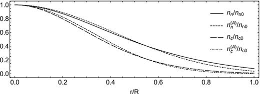
Comparison between nn/nn(0) and nc/nc(0) (obtained by numerically solving the hydrostatic equilibrium equation 16), and the simple analytical approximations |$n_\mathrm{ n}^{(A)}/n_\mathrm{ n}(0)$| and |$n_\mathrm{ c}^{(A)}/n_\mathrm{ c}(0)$|, respectively. Here, |$n_\mathrm{ n}^{(A)}$| is computed from equation (19), using |$n_\mathrm{ c}^{(A)}$|, the analytical expression for nc given by equation (20).
The transport coefficients γij(r, T) between species i and j are computed for the relations derived for τij(r, T) by Yakovlev & Shalybkov (1990), where T denotes the core temperature.
This stellar model, although very simplified, allows us to capture the effects of radial density gradients, gravity, and stable stratification into our simulations, which is a vast improvement over paper I, where the background densities were treated as fixed radially independent numbers.
2.3 Linearization
Since the density perturbations are small, we can linearize δμn = Knnδnn (where Knn = dμn/dnn), and δμc = Kccδnc (where Kcc = dμc/dnc). In our model, as there are no strong interactions, the cross-derivatives Kcn = ∂μc/∂nn and Knc = ∂μn/∂nc vanish.
2.4 Boundary conditions
2.5 Axial symmetry
2.6 Time-scale estimates
2.6.1 Short-term relaxation through fictitious friction
In order to mimic the quick hydro-magnetic relaxation due to the propagation and damping of sound waves, gravity waves, and Alfvén waves, which happens much faster than ambipolar diffusion, the fictitious friction parameter introduced in equation (2) must satisfy ζ ≪ γcnnc, so a net force imbalance on a fluid element (in round brackets on the right-hand side of equation 24) is reduced by bulk motions (with velocity |$\boldsymbol{v}_\mathrm{ n}$|) much more quickly than an imbalance of the partial forces on the charged-particle component (in round brackets on the right-hand side of equation 25) is reduced by ambipolar diffusion (with relative velocity |$\boldsymbol{v}_{\mathrm{ ad}}$|). Thus, for an arbitrary, non-equilibrium initial condition, the dynamics is initially dominated by a bulk motion with the neutron velocity, |$\boldsymbol{v}_\mathrm{ n}$|. For a characteristic spatial scale L ≲ R of the magnetic field, the time-scales for the evolution of the density perturbations, ∼(δnn/nn)(L/vn) (from equation 22) and ∼(δnc/nc)(L/vn) (from equation 23) are much shorter than that for the magnetic field, ∼L/vn (from equation 21). Thus, for t ≪ L/vn, the magnetic field can be regarded as fixed, and only the density perturbations evolve.1
These arguments remain valid when removing the restriction of axial symmetry. As two gradient forces can only balance two different components of the magnetic force (in a time-scale tζg), one component will always remain unbalanced. Therefore, reaching a state of hydro-magnetic quasi-equilibrium will always require the magnetic field to adjust so that the latter component vanishes, which will happen on a time-scale ∼tζB. Since we are interested in an evolution on a time-scale many orders of magnitude longer than an Alfvén-like time, we only need ζ to be small enough to make tζB sufficiently short to maintain the hydro-magnetic quasi-equilibrium discussed above.
Gusakov, Kantor & Ofengeim (2017) used the time-derivative of the toroidal component of the quasi-equilibrium condition, |$\partial \boldsymbol{f}_B^{\mathrm{Tor}}/\partial t=0$|, to obtain the macroscopic toroidal velocity of the particle flow. However, solving this equation at all time-steps in a simulation is unpractical, as it would require high spatial resolution to properly resolve the fourth-order derivatives over |$\boldsymbol{B}$|. Our approach is simpler, as we do not attempt to solve this equation directly, rather, we let the system relax to this condition through the addition of the fictitious friction force.
2.6.2 Long-term evolution through ambipolar diffusion
As the magnetic force acts only on the charged particles (which are coupled to the neutrons only by collisions), it induces a slow relative motion with velocity |$\boldsymbol{v}_{\mathrm{ ad}}$| in which the magnetic field lines are carried along with the charged particles. This process slowly modifies the hydro-magnetic quasi-equilibrium, eventually reaching a state in which the magnetic force is balanced mainly by the fluid force of the charged particles, while the contribution of the neutrons becomes negligible. During this process, the magnetic field has to adjust, since it has to transition from a state in which |$\boldsymbol{f}_B^{\mathrm{Pol}}$| is balanced by the sum of two different gradients to a state in which only one gradient is available. While the charged particles diffuse through neutrons at a velocity vad ∼ B2/4|$\pi$|Lγcnncnn, the neutrons have to adjust accordingly. Therefore, the velocity of the neutrons is also controlled by γcn and independent of the value given to ζ (granted that ζ is sufficiently small, so tζB is much shorter than the ambipolar diffusion time-scale).
2.7 Dimensionless equations
In order to evolve the magnetic field in the NS core, we upgraded the code described in paper I to include the motion of neutrons and the radial density gradients, so it evolves the set of equations (42)–(49). This is done by discretizing the values of the variables over a staggered polar grid composed of Nr points inhomogeneously distributed in the radial direction inside the core and Nθ points equally spaced in the polar direction, while the external multipolar expansion of α(r, θ) is truncated to the first NExp terms. The numerical computation is done conservatively for the evolution of the toroidal magnetic field and the density perturbations of the charged particles and neutrons, using a finite-volume scheme. The time derivative of the poloidal potential is computed using finite differences, and the system is evolved to second-order accuracy in time. This scheme guarantees that the |$\boldsymbol{\nabla }\cdot \boldsymbol{B}=0$| condition, as well as the total number of particles, are conserved at all times to machine precision. Details on the numerical code can be seen in paper I.
3 RESULTS
3.1 Dependence on the artificial friction
In our model, the fictitious friction force is a device to allow the particle densities and the magnetic field configuration to reach a hydro-magnetic equilibrium on time-scales ≲tζB shorter than the ambipolar diffusion time tad, but close enough to the latter for the numerical simulation to be feasible. Thus, the friction parameter ζ needs to be chosen to satisfy this compromise, and its value should not affect the long-term evolution of the magnetic field on scales ∼tad. In order to estimate its optimal value, we compare three simulations that differ only by their value of ζ. Since the total integration time is proportional to tad/tζp = 16.45/ζb2, decreasing the values of ζ and b increases the integration time very quickly. Therefore, to keep it manageable, we perform this test with an unrealistically large value of b2, namely, 10−2. For ζ, we take the values ζ1 = 10−2, ζ2 = 10−3, and ζ3 = 10−4, which yield ratios tad/tζB = 102, 103, and 104, respectively.
Our results are summarized in Fig. 2. Panel (a) shows that during the early stages (∝tζB), there is a small adjustment of the magnetic field. This is expected, as growing the density perturbations up to |δni|/ni ∼ b2 (for i = n, c) implies spatial displacements of a fraction ∼b2 of the core radius thus the magnetic field strength is expected to be reduced by a similar fraction. We also see that, while the early dynamics is dominated by the artificial friction, the three simulations converge to the same curve at t ∼ tζB∝ζ. This can be seen more clearly in panel (b). The convergence of |$\boldsymbol{v_\mathrm{ n}}$| for simulations with very different values of ζ confirms that the scheme is indeed yielding the expected results, namely fζ∝ζ, thus reproducing the correct ‘physical’ neutron velocity on time-scales t ∼ tζB, independent of the value used for ζ (as long as it is sufficiently small). The good agreement of the three curves after this time suggests that all three values chosen for ζ are adequate for our purpose. To be on the safe side, we will use ζ ∼ 10−3 to perform long-term simulations (reaching t ∼ tad), as it still yields manageable integration times.
![Comparison of the evolution of simulations using the initial condition from equation (55) and three different values of ζ (10−2, 10−3, and 10−4), which yield the following ratios between the different relevant time-scales at the centre of the star: tζp: tζg: tζB: tad = 1: 16.45: 1645: 1.645 × 10⁵ (continuous line), =1: 16.45: 1645: 1.645 × 10⁶ (dashed), and =1: 16.45: 1645: 1.645 × 10⁷ (dotted), respectively. The vertical lines show the value of the time-scale tζB for each simulation. We show the time evolution of (a) the magnetic field $\langle \boldsymbol{B} \rangle$ in units of B0, where 〈.〉 denotes rms in the volume of the core, (b) the neutron velocity $\langle \boldsymbol{v_\mathrm{ n}} \rangle$, (c) the ambipolar diffusion velocity $\langle \boldsymbol{v_{\mathrm{ ad}}} \rangle$, and (d) the ratio $\langle \boldsymbol{\nabla }\cdot (n_i\boldsymbol{v_{i}})\rangle /\langle [\boldsymbol{\nabla }\!\times \!(n_i\boldsymbol{v_{i}})]_\phi \rangle$ for neutrons (i = n, black lines), and charged particles (i = c, grey lines).](https://oup.silverchair-cdn.com/oup/backfile/Content_public/Journal/mnras/498/2/10.1093_mnras_staa2543/1/m_staa2543fig2.jpeg?Expires=1750460163&Signature=nqrX6MMovHHA6s1muEaeScPduJ-ncjqyo4NSho5qW8jRFIOjf8OjIBO2jsDWiJv32h10bs-TCqw~dbGiYsp~mF556T~wBM6EneDsGWWNs8e1M55oBx6JmnUuAHsHsXuN9~zw1D9gB6DHb9bM4BqLmuR3CCiGu-q7ZL5LkSiUSDUazFTUW8oE9VpzrIA7JxYucBlgEfDDnQ2lP3MCOJP1CsrfLRUPvq6sDlphzXnieatmzomk3KCd4Xu3gcDOY92rMPkzFTKBXYiaswbG6TNHdJ5IYcLZGX7oFSzfK6YnpgM~FU~qLLunkJGZLiJYtcVW0iTKfEW2bzzJkOzp8R~lqA__&Key-Pair-Id=APKAIE5G5CRDK6RD3PGA)
Comparison of the evolution of simulations using the initial condition from equation (55) and three different values of ζ (10−2, 10−3, and 10−4), which yield the following ratios between the different relevant time-scales at the centre of the star: tζp: tζg: tζB: tad = 1: 16.45: 1645: 1.645 × 10⁵ (continuous line), =1: 16.45: 1645: 1.645 × 10⁶ (dashed), and =1: 16.45: 1645: 1.645 × 10⁷ (dotted), respectively. The vertical lines show the value of the time-scale tζB for each simulation. We show the time evolution of (a) the magnetic field |$\langle \boldsymbol{B} \rangle$| in units of B0, where 〈.〉 denotes rms in the volume of the core, (b) the neutron velocity |$\langle \boldsymbol{v_\mathrm{ n}} \rangle$|, (c) the ambipolar diffusion velocity |$\langle \boldsymbol{v_{\mathrm{ ad}}} \rangle$|, and (d) the ratio |$\langle \boldsymbol{\nabla }\cdot (n_i\boldsymbol{v_{i}})\rangle /\langle [\boldsymbol{\nabla }\!\times \!(n_i\boldsymbol{v_{i}})]_\phi \rangle$| for neutrons (i = n, black lines), and charged particles (i = c, grey lines).
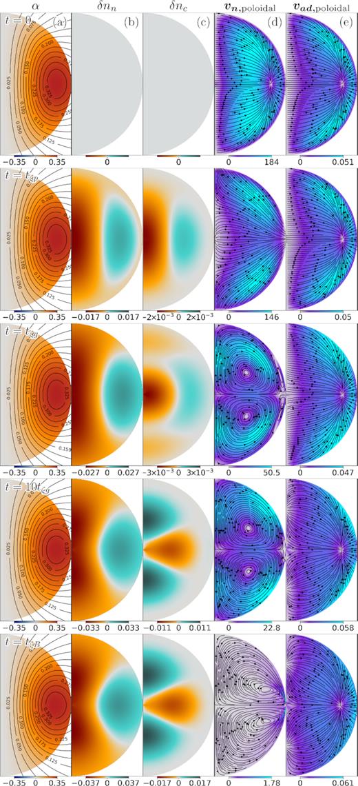
Evolution of the magnetic field discussed in Section 3.2.1, with initial conditions set by α from equation (55) and β = 0, and parameters ζ = 10−4 and b2 = 10−2, yielding time-scales at the centre of the star in proportions tζp: tζg: tζB: tad = 1: 16.45: 1645: 1.645 × 10⁷. We used a grid of Nr = 60 radial steps and Nθ = 91 polar steps inside the core, as well as NExp = 27 external multipoles. From left to right: (a) Configuration of the magnetic field, where lines represent the poloidal magnetic field and the colours the poloidal potential α; (b) and (c) density perturbations δnn and δnc, respectively, normalized to nc0; (d) and (e) poloidal component of the neutron velocity, |$\boldsymbol{v_{\mathrm{ n}}}$|, and ambipolar diffusion velocity, |$\boldsymbol{v_{\mathrm{ ad}}}$|, where arrows represent the direction and colours the magnitude normalized to R/t0. Rows correspond to different times: t = 0, tζp, tζg, 10tζg, and tζB.
It remains to be seen if the fictitious force is indeed negligible during the long-term evolution of the field, and if our estimates for the different time-scales of evolution are in agreement with our results. This will be addressed in the following section.
3.2 Hydro-magnetic evolution
3.2.1 Reaching hydro-magnetic quasi-equilibrium with a purely poloidal configuration
In this section, we study the process in which the fictitious friction rearranges the particle densities and magnetic field to reach hydro-magnetic quasi-equilibrium, checking if the associated time-scales agree with the analytical estimates of Section 2.6. For this purpose, we perform a simulation using the same initial condition as in the previous section (see equation 55). The initial condition and some snapshots of its evolution are shown in Fig. 3.
The short time-scales tζp and tζg (equations 38 and 39, respectively) are associated with a quick adjustment of the densities in the presence of a magnetic force, nevertheless they do not explicitly depend on the magnetic field strength. As they are much shorter than the time-scales for magnetic field evolution, the magnetic field remains essentially unchanged during this process. Although in our simulations we use an unrealistically high value of b, the value chosen is still small enough to understand the dynamics of the fluid motion, since tζp/tζB = 6 × 10⁻⁴. Also, here we are only interested in the dynamics on time-scales ∼tζB, thus we can use small values of ζ without changing the total integration time as the required number of time-steps will be ∝tζB/tζp, independent of ζ. Therefore, we will focus, as suggested before, on the simulation with ζ = ζ3 = 10−4.
We can see that, as expected, at short times (∼tζp), the magnetic field pushes the fluid, which grows density perturbations δnn(r, θ) and δnc(r, θ) with similar structure, in particular the same sign, as would happen in sound waves (p-modes, in asteroseismology jargon). At later times (∼tζg), although by construction the two species are still mostly moving together (as |$\boldsymbol{v_{\mathrm{ n}}} \gg \boldsymbol{v_{\mathrm{ ad}}}$|, since we are still out of quasi-equilibrium, implying |$\boldsymbol{v_\mathrm{ n}} \approx \boldsymbol{v_\mathrm{ c}}$|), their different background density profiles (nc(r)/nn(r) ≠ constant) together with a non-trivial velocity field |$\boldsymbol{v}_\mathrm{ n}(r,\theta)$| allow their continuity equations (44) and (45) to create density perturbations not necessarily of the same signs (as they would have in so-called ‘gravity waves’ or ‘g modes’, e.g. Reisenegger & Goldreich 1992), allowing their different fluid forces to jointly balance both components of the poloidal magnetic force (see panels at t = tζg and t = 10tζg). This leads joint radial motions to be opposed by strong buoyancy forces (Pethick 1992; Goldreich & Reisenegger 1992). Thus, the two components jointly behave as a single, stably stratified, non-barotropic fluid.
The strength of the magnetic and fluid forces throughout the simulation can be seen in Fig. 4. At early stages (∼tζp), the magnetic force is partially balanced by the fluid force of the neutrons, while the contribution of the charged particles is much smaller. This is because at this stage the charged particles and neutrons at any point in the star are jointly compressed or expanded by the magnetic force (with δnc(r, θ)/nc(r) ∼ δnn(r, θ)/nn(r)). Since there are many more neutrons than charged particles present, they represent the main contribution to the pressure of the fluid. At later times (∼tζg), the neutron and charged-particle density perturbations become very different and the latter also contribute substantially to the fluid force. At first, it may be surprising that the two fluid forces do not act in the same direction, opposite to the magnetic force. Instead, they grow very different density perturbations that, acting together, balance the magnetic force (see the red line). It is clear from Section 2.6.1 that to reach this kind of force balance, density perturbations of similar magnitude (but not necessarily of the same sign) are required. The relative smallness of fζ in Fig. 5(d), shows that this force balance is being reached. Nevertheless, as the magnetic flux is slowly being carried by the motion of the fluid, a perfect force balance cannot be reached, as seen in Fig. 4: After their fast initial growth (in a time-scale ∼tζg), the fluid forces reach a plateau. However, as the magnetic field evolves (on a much slower time-scale), the particles have to keep up, thus evolving at the same rate as the magnetic field, until the latter reaches a new quasi-equilibrium configuration at times ∼tζB. At this point, all forces are close to balancing, and the fictitious friction becomes negligible compared to all of the physical forces (|fζ|/min{|fB|, |fc|, |fn|}∝ζ/γcnnc). Thus, at this point the fictitious force plays no significant role in the evolution of the field, other than giving us a way of computing the neutron velocity field needed to maintain the quasi-equilibrium condition fζ ∼ 0. It is also worth noting that the topology of the velocity fields at this point is consistent with the results from Ofengeim & Gusakov (2018) (see Fig. 3d and e at t = tζB), although a quantitative comparison is not possible since our toy-model equation of state does not consider entrainment.
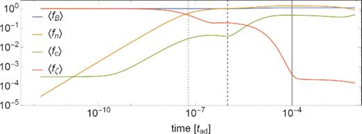
For the simulation of Fig. 3: Time evolution of the force densities |$\langle \boldsymbol{f_B} \rangle$|, |$\langle \boldsymbol{f_\mathrm{ n}} \rangle$|, |$\langle \boldsymbol{f_\mathrm{ c}} \rangle$| and |$\langle \boldsymbol{f_\zeta } \rangle$|, all of them normalized by |$\langle \boldsymbol{f_B}(t=0)\rangle$|, where 〈.〉 denotes rms in the volume of the core. Time is in units of tad. The vertical lines show, from left to right, the values of the time-scales tζp, tζg, and tζB.
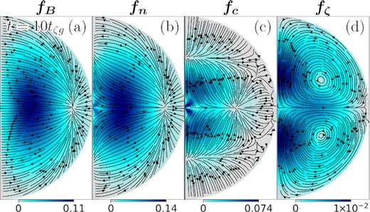
From left to right: Snapshot of (a) |$\boldsymbol{f_B}$|, (b) |$\boldsymbol{f_\mathrm{ n}}$|, (c) |$\boldsymbol{f_\mathrm{ c}}$|, and (d) |$\boldsymbol{f_\zeta }$| for the simulation of Fig. 3 at t = 10tζg. Arrows represent the direction of the forces at each point, and colours their magnitudes.
3.2.2 Long-term magnetic field evolution of a poloidal and toroidal configuration
In the previous sections, we studied simulations of a purely poloidal magnetic field, which is known to be unstable to non-axisymmetric perturbations (Markey & Tayler 1973; Flowers & Ruderman 1977; Marchant, Reisenegger & Akgün 2011). Thus, in order to study the long-term evolution, we now consider a simulation for the much more realistic case of a field with poloidal and toroidal components. This allows us to check whether the time-scales for the magnetic field evolution from Section 2.6 (equations 40 and 41) are in agreement with our numerical scheme, but mainly, it allows us to study the impact of the neutron motions on the long-term evolution of the magnetic field.
The initial configuration, as well as some snapshots of its evolution, are shown in Fig. 6. We see how at t = tζp the density perturbations grow together following δnc/nc ∼ δnn/nn, while at t = tζg they are evolving towards a state in which their signs are not correlated, thus reproducing the results from the previous section. This can also be observed in Fig. 7(a), which shows the rms of the different fluid forces throughout the simulation. During the first stages of the evolution (t ∼ tζp–tζg), the magnetic force is partially balanced by the fluid forces, which are dominated by the neutrons.
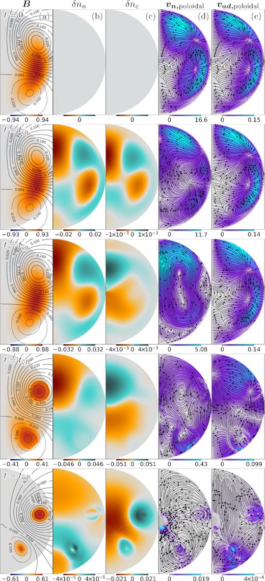
Evolution of the magnetic field discussed in Section 3.2.2 with initial conditions given by equations (59) and (60) (so the poloidal component has 60 per cent of the initial internal magnetic energy), and parameters ζ = 3 × 10⁻³ and b2 = 10−2. Thus, the time-scales at the centre of the star satisfy tζp: tζg: tζB: tad = 1: 16.45: 1645: 548500. We used a grid of Nr = 60 radial steps and Nθ = 91 polar steps inside the core, as well as NExp = 27 external multipoles. From left to right: (a) Configuration of the magnetic field, where lines represent the poloidal magnetic field (labelled by the magnitude of α) and colours the toroidal potential β; (b) and (c) density perturbations δnn and δnc, respectively, both normalized to nc0; (d) and (e) poloidal component of the neutron velocity, |$\boldsymbol{v_\mathrm{ n}}$|, and ambipolar diffusion velocity, |$\boldsymbol{v_{\mathrm{ ad}}}$|, where arrows represent the direction and colours the magnitude normalized to R/t0. Rows correspond to different times: t = 0, tζp, tζg, tζB, and tad.
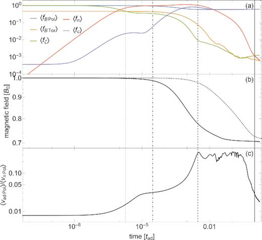
For the simulation of Fig. 6: Time evolution of (a) the rms force densities |$\langle \boldsymbol{f_{B\, \text{Pol}}} \rangle$|, |$\langle \boldsymbol{f_{B\, \text{Tor}}} \rangle$|, |$\langle \boldsymbol{f_\mathrm{ n}} \rangle$|, |$\langle \boldsymbol{f_\mathrm{ c}} \rangle$|, and |$\langle \boldsymbol{f_\zeta } \rangle$|, all normalized by |$\langle \boldsymbol{f_{B\, \text{Pol}}}(t=0)\rangle$|, where 〈.〉 denotes rms in the volume of the core; (b) the rms magnetic field |$\langle \boldsymbol{B} \rangle$| (in units of its initial value B0) in the NS core. The dotted line corresponds to |$\langle \boldsymbol{B} \rangle$| on a simulation using the same initial condition, but taking ζ → ∞ (fixed neutrons); and (c) |$\langle v_{\mathrm{ ad}\, \text{Pol}}\rangle /\langle v_{n\, \text{Pol}}\rangle$|. For all panels, time is in units of tad. The vertical lines show, from left to right, the time-scales tζp, tζg, tζB, and tad.
In the fourth row of Fig. 6 (at t = tζB), it can be seen how the magnetic field unwinds, eliminating most of the toroidal component, except in the regions of closed poloidal field lines. As discussed in paper I, such ‘twisted-torus’ configurations are expected in axially symmetric hydro-magnetic equilibria, because there is no toroidal pressure gradient or gravitational force available to balance a toroidal component of the Lorentz force. This implies the restriction β = β(α) on the potentials, which is also verified in the figure (see also Fig. 8). This state corresponds to a non-barotropic quasi-equilibrium, as both charged particles and neutrons, which have different fluid forces, are contributing to balance the magnetic force. This can be seen more clearly in Fig. 7(a), where the poloidal magnetic force and fluid forces are all of the same order, but the poloidal force imbalance |$\langle \boldsymbol{f_{\zeta ,\text{Pol}}} \rangle$| is much smaller, meaning that in the poloidal component there is a balance between the magnetic force and the induced fluid forces. In the toroidal component, |$\boldsymbol{f_{\zeta ,\text{Tor}}}=\boldsymbol{f_{B,\text{Tor}}}$| always, but at tζB this force has become much smaller than its initial value. Thus, the configuration at t ∼ tζB is very close to a (non-barotropic) hydro-magnetic quasi-equilibrium where even the toroidal component of friction force has become small.
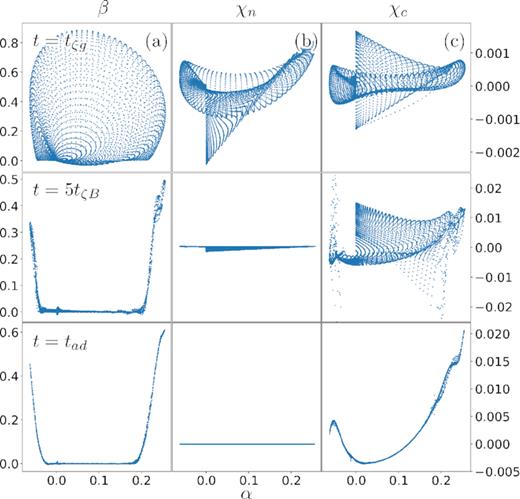
For the simulation of Fig. 6: Scatter plot of α versus (a) β, (b) χn, and (c) χc, showing all of the grid points at t = tζg, t = 5tζB, and t = tad, respectively. The axis label on the left side of the figure corresponds to plot (a), while that on the right corresponds to (b) and (c).
On a much longer time-scale, this quasi-equilibrium is slowly eroded by ambipolar diffusion. Charged particles, pushed by the magnetic force, carry the magnetic flux relative to the neutrons until the magnetic force can be balanced by the force due to the density perturbations of the charged particles alone, choking the motion. This can be seen in the last row of Fig. 6 (t = tad), where the ambipolar velocity is much smaller than at tζB. Also, |δnc|/nc ≫ |δnn|/nn, confirming that the magnetic force is mostly balanced by the charged particles. This is further supported by Fig. 7(a), which shows a transition from t = tζB, where the magnetic force is balanced by the combined force from charged particles and neutrons, to t = tad, where it is balanced mostly by the charged particles, while the contribution from the neutrons becomes negligible.
However, this does not mean that the neutron motion is irrelevant to the long-term evolution. While ambipolar diffusion pushes the charged particles relative to the neutrons, all components (neutrons, charged particles, and the magnetic field) have to keep adjusting to successive quasi-equilibria, thus inducing a slow macroscopic motion of the fluid. This motion (controlled by the drag force between neutrons and charged particles) gives the charged particles an extra push, shortening the time-scale for the long-term magnetic evolution (∼L/vc). This can be seen in Fig. 7(b), where the decay of the magnetic field in the simulation with mobile neutrons is much faster than in a simulation with the same initial condition, but with fixed neutrons.
As discussed in Section 2.6, we expect that in the quasi-stationary state |∂δnc/∂t| is much smaller than both |$|\boldsymbol{\nabla }\cdot \left(n_\mathrm{ c}\boldsymbol{v_{\mathrm{ ad}}}\right)|$| and |$|\boldsymbol{\nabla }\cdot \left(n_\mathrm{ c}\boldsymbol{v_\mathrm{ n}}\right)|$|. Thus, the irrotational components of |$n_\mathrm{ c}\boldsymbol{v_\mathrm{ n}}$|, and |$n_\mathrm{ c}\boldsymbol{v_{\mathrm{ ad}}}$| are of the same order. However, as pointed out in Section 3.1, both vector fields are dominated by their solenoidal component, and Fig. 7(c) shows that, during the long-term evolution from tζB to tad, vn becomes larger than vad by a factor ∼4. Similar fractions were found for different simulations in our tests. This is in agreement with the results of Ofengeim & Gusakov (2018). In Fig. 7(c) we also see that, towards the end on the simulation, the core is reaching equilibrium, thus |$\boldsymbol{v_{\mathrm{ ad}}}$| gets progressively smaller, faster than |$\boldsymbol{v_\mathrm{ n}}$|. Sadly, at this point the numerical noise starts to become dominant towards the centre of the star, where the coordinate system is singular (see Fig. 6[d] at t = tad).
3.3 Grad–Shafranov equilibria
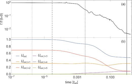
For the simulation of Fig. 6: Time evolution of (a) the ‘Grad–Shafranov integral’ Γ (defined in equation 66) and (b) the magnetic energy stored in the ℓ-th component of the external magnetic field (see equation 31). The vertical lines show, from left to right, the time-scales tζp, tζg, tζB, and tad.
4 CONCLUSIONS
In paper I, we studied the long-term evolution of the magnetic field of an NS through ambipolar diffusion, modelling its core as a charged-particle fluid of protons and electrons, which carries the magnetic flux through a motionless uniform background of neutrons. In this paper, we addressed two of the main shortcomings of that work by allowing neutrons to move as well as including different density gradients for neutrons and charged particles, thus accounting for their stable stratification.
We know that the star can reach a hydro-magnetic quasi-equilibrium many orders of magnitude faster than the magnetic field evolution time-scales. To maintain quasi-equilibrium realistically during the evolution of the field would require following the propagation of sound, gravity, and Alfvén waves. Resolving such processes would make it impossible to simulate the long-term evolution of the field. We have addressed this issue by adding a fictitious friction force to the equation of motion of the neutrons (Hoyos et al. 2008). This force, which causes a neutron velocity proportional to the net force imbalance at each point, replaces the very small inertial terms present in the equations of motions, and provides a mechanism to maintain the hydro-magnetic quasi-equilibrium.
Our results can be summarized as follows:
The addition of the fictitious friction in our simulations was found to be a useful method to quickly reach and then maintain the hydro-magnetic quasi-equilibrium of the star without having to resolve the propagation of sound, gravity, and Alfvén waves, leading to the same kind of non-barotropic ‘twisted torus’ quasi-equilibrium previously found in MHD simulations (Braithwaite & Spruit 2004; Braithwaite & Nordlund 2006) in a time-scale tζB that can be adjusted to make the simulations both doable and physically interesting.
We found good agreement between different expected time-scales involved in this process (tζp, tζg, and tζB), and simulations. The long-term evolution of the magnetic field is not significantly affected by the fictitious friction force if the ratio between the time-scale in which the hydro-magnetic quasi-equilibrium is restored by this artificial friction and the time-scale of ambipolar diffusion is small enough (tζB/tad ∼ ζ/γcnnc ≲ 10−3 in our simulations).
- Relaxing the unrealistic assumption of fixed neutrons was found to impact the long-term evolution of the magnetic field in the following way: Since the density profiles of neutrons and charged particles are different, joint motion of the two species is strongly constrained by buoyancy forces. Thus, there will always be relative motions between species (i.e. ambipolar diffusion). This process, in which the magnetic force pushes the charged particles and magnetic flux relative to the neutrons, slowly erodes the hydro-magnetic quasi-equilibrium; therefore neutrons, charged particles, and the magnetic field have to continuously adjust to restore it. This motion makes the charged particles (and thus the magnetic flux) move faster than in the case of fixed neutrons, thus shortening the time-scale for magnetic evolution. In our simulations we find that the speed of neutrons and charged particles can be ∼1–10 times larger than their relative velocity, yielding a time-scalefor the long-term evolution of the field.(67)$$\begin{eqnarray*} t_{\mathrm{ ad}} \sim (0.3 - 3)\times 10^{3} \, \left(\frac{10^{15}\text{G}}{B}\right)^{2}\left(\frac{T}{10^8\,\text{K}}\right)^{2}\left(\frac{L}{1\,\text{km}}\right)^{2}\, \text{yr} \end{eqnarray*}$$
The process described above leads to a final equilibrium state in which the magnetic force is balanced by the pressure and gravitational forces of the charged particles, while the neutron density perturbations become negligible, thus recovering the barotropic ‘Grad–Shafranov equilibria’ from paper I.
The following two main caveats need to be addressed by future work:
It is likely that the magnetic equilibria found may become unstable if we relax the axial symmetry restriction, as previous works indicate that there are no stable hydro-magnetic equilibria in barotropic stars (Braithwaite 2009; Akgün et al. 2013; Mitchell et al. 2015). In that case ambipolar diffusion might dissipate all the magnetic flux, so the low magnetic field of millisecond pulsars might be explained by magnetic flux dissipation prior to accretion (Cruces et al. 2019). However, if the charged particles also include muons, the charged fluid will no longer be barotropic, which may help to stabilize the magnetic field.
NS matter is expected to be superfluid and superconducting at the temperatures of interest, which might have a major impact on the time-scales described here, as the coupling between the different species should, in principle, be many orders of magnitude smaller. The dynamics of the field evolution might also be quite different from what we presented here, as the macroscopic effect of the dynamics and interactions between quantized neutron vortices and magnetic flux tubes needs to be taken into account.
In this work, we assumed a potential solution for the crustal and external magnetic field, thus assuming that the crust adjusts instantaneously to the evolution in the core. However, if the crust is highly conductive, this may not be the case as currents may keep circulating in the crust, leading to non-trivial configurations (see for instance Cumming, Arras & Zweibel 2004; Pons & Geppert 2007; Gourgouliatos, Wood & Hollerbach 2016; Akgün et al. 2018). Ultimately, this might indicate that it is the crust which sets the time-scale for the evolution of the external field, leading to more restrictive equilibrium configurations in the core.
ACKNOWLEDGEMENTS
We are very grateful to M. Gusakov, J. Pons, and the ANSWERS group in Santiago de Chile for useful discussions. This work was supported by the National Fund for Scientific and Technological Development (FONDECYT) projects 3180700 (FC), 1201582 (AR), and 1190703 (JAV), and the Center for Astrophysics and Associated Technologies (CATA; CONICYT/ANID project Basal AFB-170002). JAV thanks for the support of the Center for the Development of Nanoscience and Nanotechnology (CEDENNA) under CONICYT/ANID grant FB0807.
DATA AVAILABILITY
The data underlying this article will be shared on reasonable request to the corresponding author.
Footnotes
Formally, equations (22) to (30) can be rewritten as a system of two coupled diffusion equations for δnn and δnc with an inhomogeneous term linear in |$\boldsymbol{f_B}$| (which can be taken as a constant in this regime) and diffusion coefficients (and thus characteristic time-scales) independent of |$\boldsymbol{B}$|.
