


ABSTRACT
We present the hestia simulation suite: High-resolutions Environmental Simulations of The Immediate Area, a set of cosmological simulations of the Local Group. Initial conditions constrained by the observed peculiar velocity of nearby galaxies are employed to accurately simulate the local cosmography. Halo pairs that resemble the Local Group are found in low resolutions constrained, dark matter only simulations, and selected for higher resolution magneto hydrodynamic simulation using the arepo code. Baryonic physics follows the auriga model of galaxy formation. The simulations contain a high-resolution region of 3–5 Mpc in radius from the Local Group mid-point embedded in the correct cosmographic landscape. Within this region, a simulated Local Group consisting of a Milky Way and Andromeda like galaxy forms, whose description is in excellent agreement with observations. The simulated Local Group galaxies resemble the Milky Way and Andromeda in terms of their halo mass, mass ratio, stellar disc mass, morphology separation, relative velocity, rotation curves, bulge-disc morphology, satellite galaxy stellar mass function, satellite radial distribution, and in some cases, the presence of a Magellanic cloud like object. Because these simulations properly model the Local Group in their cosmographic context, they provide a testing ground for questions where environment is thought to play an important role.
1 INTRODUCTION
Astronomers and astrophysicists have long used nearby objects as guides for understanding more distant ones. The Earth is often taken as a paradigmatic rocky planet, the Sun as a model star, and the Milky Way (MW) as an archetypal spiral galaxy. This pedagogy is natural given that the Earth, the Sun, and the Galaxy are observed in much greater detail than their more distant counterparts. However, such an approach will always beg the questions: how prototypical are these objects? How responsible is it to extrapolate what we learn here, to there? Just because they are near and lend themselves naturally to the kind of observation one can only dream of obtaining elsewhere, need not mean they are representative of their astronomical object ‘class’ as a whole. Such a debate constitutes the essence of an observational science.
Furthermore, a number of observations of the MW have recently exacerbated claims that perhaps it is unusual. However (driven by the underlying axiom of our field), cosmologists are loathe to invoke any anti-Copernican explanation for confusing observations. Specifically, many of the satellites of the MW – small dwarf galaxies many with low surface brightness that orbit inside its dark matter halo, have posed a number of questions that remain either fully or partially unresolved. For example, the ‘classical’ dwarf galaxies are distributed in a highly anisotropic ‘Great Pancake’ (Kroupa, Theis & Boily 2005; Libeskind et al. 2005) or ‘disc of Satellites’ (see Pawlowski 2018, for a review). Another satellite issue was highlighted by Geha et al. (2017) who found that the MW’s satellite population, when compared with observational ‘analogues’ (based on K-band luminosity), have significantly lower star formation rates than expected. The so-called ‘Missing satellite’ problem (Klypin et al. 1999; Moore et al. 1999) is perhaps the most (over) studied of these and refers to the overprediction of dark matter satellites in the Λ cold dark matter (ΛCDM) model of structure formation, when compared with the bright observed satellites of the MW (for a non-exhaustive list of possible remedies see Efstathiou 1992; Benson et al. 2002; Knebe et al. 2002; Lovell et al. 2012; Brooks et al. 2013; Sawala et al. 2016a,b). Similarly, Boylan-Kolchin, Bullock & Kaplinghat (2011b) showed that the internal densities of the most massive simulated substructures around MW mass haloes is too large that they cannot have been rendered ‘dark’ via reionization or photoevaporation processes, but these are not observed. It is clear that in the dwarf galaxies regime, objects that are best observed in the Local Group (LG), a number of discrepancies with theoretical predictions have been found.
The problem may be that the starting point for such studies is to assume the MW is a proto-typical galaxy that lives in an |$\sim 10^{12}\, \mathrm{M}_{\odot }$| halo. This may or may not be the case. What is known is that galaxy evolution is regulated by environment either via merger rates or the availability of a gas reservoir from which stars may form. Dressler (1980) first pointed out that redder early-type galaxies consisting of older stellar populations tend to reside in more dense regions than bluer late-type discs. Galaxies in voids are about 30 per cent more metal poor than the general population (Pustilnik, Tepliakova & Kniazev 2011). It is also empirically evidenced that neighbouring galaxies have correlated specific star formation rates (Weinmann et al. 2006; Kauffmann, Li & Heckman 2010; Kauffmann et al. 2013; Knobel et al. 2015), a phenomenon termed galactic conformity (see also Hearin, Behroozi & van den Bosch 2016). Galaxy spin and angular momentum is also well known to be shaped by environment (see Navarro, Abadi & Steinmetz 2004; Tempel & Libeskind 2013; Pahwa et al. 2016; Wang & Kang 2017; Laigle et al. 2018; Ganeshaiah Veena et al. 2019, among others). The so-called nature versus nurture debate can be summarized as: how does environment regulate galaxy formation and evolution?
In order to address these questions in the context of the LG one must, of course, simulate galaxy systems that resemble the LG. The most common (albeit slightly simplistic) approach is to simulate pairs of galaxies. Studies such as Garrison-Kimmel et al. (2014), Sawala et al. (2016b), and Fattahi, Navarro & Frenk (2020b), among others have investigated pairs of galaxies that resemble the LG geometrically and physically. Often the results suggest that the nature of the LG itself is not enough to account for differences between isolated MW-like haloes and paired ones.
But where these studies fall short is that the environment – the cosmographic landscape – is not accounted for. Namely such studies produce LG-like pairs in uncontrolled, random environments. However our cosmographic landscape – a supergalactic plane, the existence of the Virgo Cluster, a filament funnelling material towards it, the evacuation from the local void, all influence the formation of the LG. Libeskind et al. (2015, 2019) suggested that the planes of satellites observed in the LG are aligned with the reconstructed large-scale structure, hinting at a causal relationship. Similarly Shaya & Tully (2013) pointed towards the relationship between planes of satellites and evacuation from the Local Void (see Hoffman et al. 2018; Tully et al. 2019). McCall (2014) found evidence, via a ‘council of giant’ galaxies, that the LG is dynamically connected to its local environment (see also Neuzil, Mansfield & Kravtsov 2020) that stretches well into the quasi-linear regime (3–5 Mpc) and is influenced by linear scales as well (i.e. the Virgo cluster, see Lee & Lee 2008). Libeskind et al. (2011) showed that satellites are accreted from the direction pointing to the Virgo cluster in simulations, later confirmed more generically in the context of tidal forces (Libeskind et al. 2014; Kang & Wang 2015; Wang & Kang 2018, see also Kubik et al. 2017). These studies (and more) have emphasized the importance for the local cosmography on the formation of the LG, and the MW.
A commitment to modelling the environment in studies of the LG was made by the clues collaboration1 (Gottlöber, Hoffman & Yepes 2010; Libeskind et al. 2010; Carlesi et al. 2016; Sorce et al. 2016a) that recognized this often overlooked aspect of most theoretical studies of the LGs. Simulations emanating from the clues collaboration have already demonstrated the importance of environment in studies which, for example, focused on the preferred directions of accretion (Libeskind et al. 2011), the trajectory of backsplash galaxies (Knebe et al. 2011), LG mass estimators (Di Cintio et al. 2012), cosmic web stripping of LG dwarfs (Benítez-Llambay et al. 2013), and the reionization of the LG (Ocvirk et al. 2013, 2014; Dixon et al. 2018). The purpose of this paper is to combine a contemporary magento-hydrodynamic (MHD) treatment of cosmic gas with the state-of-the-art Auriga galaxy formation model (Grand et al. 2017) run on initial conditions (ICs) constrained by cosmographic observations thus destined to produce an object that resembles the LG in two important ways: internally (MW and M31-type galaxies, at the correct separation, etc.) and externally (the correct large-scale structure).
The simulations presented2 here thus constitute an extension and improvement on a canon of previous work. A number of improvements have been made regarding the constrained simulation algorithm, the MHD galaxy formation models, as well as the input data. These are the first hydrodynamic zoom-in, z = 0 simulations run on ICs constrained by peculiar velocities presented in the CosmicFlows-2 catalogue (Tully et al. 2013, see Section 2.1). The CosmicFlows data base and catalogue have been used extensively before to study the local Universe, including the cold spot repeller (Courtois et al. 2017), the Vela super cluster (Courtois et al. 2019), the bulk flow (Hoffman, Courtois & Tully 2015), and the Virgo cluster (Sorce et al. 2016c; Olchanski & Sorce 2018; Sorce, Blaizot & Dubois 2019). As will be demonstrated below, producing such constrained simulations is not trivial but will provide an optimum testing ground for understanding both the role of our environment in shaping the LG as well as the holistic formation of LG galaxies.
2 MODELLING AND SIMULATION METHOD
This section includes background material on the constrained simulation method, the MHD, and the galaxy formation algorithm.
2.1 Wiener filter reconstructions, cosmic flows, and IC generation
In this section, the technique used to generate ICs that are on one hand consistent with the ΛCDM prior, and on the other constrained by observational data to reproduce the bulk cosmographic landscape of the local Universe, are explained. For a comprehensive pedagogical explanation of the technique tersely summarized and augmented below, the reader is referred to Hoffman (2009).
In the paradigm adopted here – the ΛCDM model – structures form via gravitational instability. At high redshifts, the (over)density and peculiar velocity fields constitute Gaussian random fields of primordial fluctuations (i.e. Zel’Dovich 1970; Bardeen et al. 1986). The emergence of non-linear structure via gravitational instability drives the large-scale structure away from Gaussianity, yet on scales down to a few Mpc the velocity field remains close to being a Gaussian random field. It follows that given a measurement of the peculiar velocity field, the linear Bayesian tool of the Wiener Filter (WF) and Constrained Realizations (CR) (Hoffman & Ribak 1991; Zaroubi et al. 1995) are optimal for the reconstruction of the large-scale structure and peculiar velocities (Zaroubi, Hoffman & Dekel 1999).
2.1.1 Sampling
The process of generating constrained ICs commences with sampling of the peculiar velocity field via direct measurements of galaxy distances and redshifts. Peculiar velocities are then obtained by vpec = vtot − H0 × d, where d is the measured distance, H0 is the Hubble expansion rate today, and vtot is the total velocity of the galaxy with respect to the CMB. In the following, we use the publicly available CosmicFlows-2 (CF2) catalogue (Tully et al. 2013), which consists of over 8000 direct distance measurements, out to a distance of ∼250 Mpc. The median distance of the catalogue is ∼70 Mpc.
2.1.2 Grouping
The CF2 catalogue includes a considerable number of galaxies that are members of groups and clusters, the velocities of which are affected by small-scale non-linear virial motions. Grouping these galaxies − namely collapsing data points identified as belonging to the same group or cluster into a single data point, provides an effective remedy to the problem (Sorce, Hoffman & Gottlöber 2017) as it filters the non-linear component of the large scale velocity field. Here we have used the original grouping proposed for CF2 (Tully, private communication). This grouping reduces the size of the CF2 catalogue to 4837 data points.
2.1.3 Bias minimization
It is well known that observational catalogues are inherently biased, often referred to as ‘Malmquist’ bias (e.g. see section 6.4 of Strauss & Willick 1995). One of the main issues dealt with here is that the observational error is on the distance modulus which, when converted in to a distance, translates in to a lognormal error distribution. This often leads to spurious infall in the absence of simulated galaxy clusters, if not properly corrected. Different types of biases have been discussed in Sorce (2015) where an iterative method to minimize the spurious infall on to the Local Volume, to reduce non-Gaussianities in the radial peculiar velocity distribution and to ensure the correct distribution of galaxy clusters (including our closest cluster, Virgo; see Sorce et al. 2016c; Sorce 2018), has been designed applied. The result is a new distribution of radial peculiar velocities, their uncertainties and corresponding distances. This distribution has been used in the next steps.
2.1.4 Displacement corrections
The WF/CRs algorithm and the linear mapping to the young universe are done within the Eulerian framework, in which displacements are neglected. Yet, the growth of structure involves the displacements of mass elements over cosmological time – in first approximation the so-called Zeldovich displacements. The reversed Zeldovich approximation has been devised to undo these displacements and is applied here to bring back the data points close to their primordial positions with the 3D reconstructed cosmic displacement field (Doumler et al. 2013; Sorce et al. 2014).
2.1.5 Constrained initial conditions
Density fields constrained by these modified observational peculiar velocities are constructed using the CR/WF technique (Hoffman & Ribak 1991; Zaroubi et al. 1999). At this step, the grouped and bias minimized peculiar velocity constraints are applied to a random (density and velocity) realization used to restore statistically the unconstrained structures. In fact, in the presence of the very noisy and incomplete velocity data the WF alone would provide no density fluctuations at all in most parts of the simulation volume (where there is no data the WF returns the mean field). Finally, the density fields are rescaled to build constrained ICs in the simulation box.
2.1.6 Small-scale power
Structures on scales smaller than that of shell-crossing are predominantly random and are not directly affected by the imposed constraints. The desired reconstructed LG lies within this random domain and while its structure is not directly constrained by the CF2 data, the boundary conditions on the LG and the tidal field that affects it are strongly constrained by the data. The construction of the ICs for the hestia LG is decomposed into the construction of the long waves by the CR/WF algorithm described above and adding of short waves as random realizations assuming the same ΛCDM power spectrum (Carlesi et al. 2016). Naturally, not all of these random realization contain an object that could be identified as an LG. In Section 3.2, we describe the identification algorithm for the ICs of the high-resolution LG candidates.
2.2 Simulation code
In this section, we summarize the properties of the arepo code we use and the auriga galaxy formation model. A publicly available version of the arepo code is available (Weinberger, Springel & Pakmor 2019).3
2.2.1 Magnetohydrodynamics with the moving-mesh code arepo
The arepo code (Springel 2010; Pakmor et al. 2016) solves the ideal magnetohydrodynamics (MHD) equations on an unstructured Voronoi-mesh with a second-order finite-volume scheme. The Voronoi mesh is generated from a set of mesh-generating points, each of them creating one cell. The mesh-generating points move with the gas velocity, which reduces the mass flux over interfaces and the advection errors compared to static mesh codes, making the code quasi-Lagrangian. In addition, mesh-generating points of highly distorted cells are slowly moved towards their cell centres to make sure that the mesh stays regular (Vogelsberger et al. 2013). Additional explicit refinement and derefinement is used to control the properties of the cells where appropriate. By default, the mass of each cell is kept within a factor of 2 of a target mass resolution. However, arepo in general allows for additional refinement criteria, e.g. to set a minimum cell size in the circumgalactic medium (van de Voort et al. 2019).
The fluxes over interfaces are computed in the moving frame of the interface using the HLLD Riemann solver (Pakmor, Bauer & Springel 2011; Pakmor & Springel 2013). The divergence of the magnetic field is controlled with the 8-wave scheme (Powell et al. 1999). Time integration is done via a second-order accurate scheme. arepo allows a hierarchy of time-steps below the global time-step, such that every resolution element is integrated on the time-step required by its own local time-step criterion (Springel 2010).
Self-gravity and other source terms are coupled to the ideal MHD equations by operator splitting. Gravitational forces are computed using a hybrid TreePM technique (Springel 2005) with two Fourier mesh levels, one for the full box and one centred on the high-resolution region (see below).
2.2.2 The Auriga galaxy formation model
The Auriga galaxy formation model (Grand et al. 2017), which is based on the Illustris model (Vogelsberger et al. 2013), implements the most important physical processes relevant for the formation and evolution of galaxies. It includes cooling of gas via primordial and metal cooling (Vogelsberger et al. 2013) and a spatially uniform UV background (Vogelsberger et al. 2013). The interstellar medium is described by a subgrid model for a two-phase medium in which cold star-forming clouds are embedded in a hot volume-filling medium (Springel & Hernquist 2003). Gas that is denser than nthres = 0.13 cm−3 forms stars following a Schmidt-type star formation law. Star formation itself is done stochastically and creates star particles with the target gas mass that represent single stellar populations (SSPs). The model includes mass-loss and metal return from asymptotic giant branch (AGB) stars, core-collapse supernovae, and Type Ia supernovae that are distributed in the cells around a star particle.
Galactic winds are implemented by creating a wind with a given velocity and mass loading just outside the star-forming phase. At the technical level, this non-local momentum feedback is realized by creating temporary wind particles that are launched isotropically from sites of star formation, dumping their momentum, mass and energy into a local cell once they encounter gas with a density less than |$0.05\, n_\mathrm{thres}$| (Grand et al. 2017). Despite being launched isotropically, this model generates coherent bipolar outflows for disc galaxies at low redshift (Grand et al. 2019; Nelson et al. 2019). The Auriga model also follows the formation and growth of supermassive black holes and includes their feedback as active galactic nuclei (AGNs).
Magnetic fields are seeded as uniform seed fields at z = 127 with a comoving field strength of 10−14 G. As the magnetic fields in galaxies are quickly amplified by an efficient turbulent dynamo at high redshift (Pakmor, Marinacci & Springel 2014; Pakmor et al. 2017) they lose any memory of the initial seed field of the simulation. Note however, that the magnetic field between galaxies reflects the initial the seed field, and is therefore not a prediction of the simulations (Marinacci et al. 2015).
The Auriga model has been used successfully to study a large number of questions on the formation and evolution of Milky Way-like galaxies and their satellite galaxies. It reproduces many general properties of the stellar component of Milky Way-like galaxies (Grand et al. 2017, 2018), as well as their gas (Marinacci et al. 2017), their stellar halo (Monachesi et al. 2019), and their satellite systems (Simpson et al. 2018; Fattahi et al. 2020a). Moreover, the evolution of the magnetic fields in the disc and the circum-galactic medium has been studied extensively for the Auriga simulations and found to be in excellent agreement with observations of the Milky Way and other nearby disc galaxies (Pakmor et al. 2017, 2018, 2020).
Finally, the Auriga model is very similar in the mass range of Milky Way-like galaxies to the IllustrisTNG model (Weinberger et al. 2017; Pillepich et al. 2018) that has been found to quite successfully reproduce the properties of the full galaxy population in a representative part of the universe (see e.g. Springel et al. 2018).
3 ANALYSIS
All simulations in this work assume a cosmology consistent with the best-fitting Planck Collaboration XVI (2014) values: σ8 = 0.83 and H0 = 100h km s−1 Mpc−1, where h = 0.677. We adopt ΩΛ = 0.682 throughout; for DM only runs ΩM = 0.318, while for hydrodynamic runs ΩM = 0.270 and Ωb = 0.048.
3.1 Post-processing of the simulation output
In this section, the post-processing halo finder (and accompanying tools) that are used throughout this work to identify haloes, subhaloes, galaxies, and merger history are described. In addition to the friends-of-friends (FOF) catalogues (used exclusively for seeding the Black Hole’s in the galaxy formation model), haloes and subhaloes are also identified at each redshift by using the publicly available ahf4 halo finder (Knollmann & Knebe 2009). ahf identifies local overdensities in the adaptively smoothed density field as prospective halo centres. The local potential minimum is computed for each density peak and the particles that are gravitationally bound are identified. The thermal energy of the gas is used in the unbinding procedure by simply adding it to the total specific energy, which is required to be negative. Only peaks with at least 20 bound particles are considered as haloes and retained for further analysis. ahf automatically identifies haloes, subhaloes, sub-subhaloes, etc.
Magnitudes and colours are computed via a stellar population synthesis model called stardust (see Devriendt, Guiderdoni & Sadat 1999, and references therein for a detailed description). This is used to derive the luminosities from the star particles (i.e. SSP) in each halo. stardust additionally computes the spectral energy distribution from the far-UV to the radio, for an instantaneous starburst of a given mass, age, and metallicity.
Galaxy and halo histories are estimated via merger trees. A tool (aptly named mergertree) is included as part of the ahf package for this purpose. At each redshift accretion events are found by identifying which subhaloes at a given snapshot are identified as ‘field’ haloes at the previous snapshot. Haloes may also grow via smooth accretion from the environment, namely via gravitationally attracting particles in their vicinity.
Thus, the data obtained and retained from the simulation for further analysis consists not just of the raw simulation output, namely the position, velocity, mass, and baryonic properties (where applicable) of the particles and cells, but the (sub-)halo finder’s ahf catalogue, with bulk baryonic properties computed, as well as merger trees and halo growth data. Throughout this paper only the ahf post-processing output is used.
3.2 Identification of Local Groups
3.2.1 Low-resolution runs
As explained in Section 2.1, each constrained realization requires two random seeds. One source of randomness is associated with the unconstrained regions and the incompleteness of the sampling (including the finite size of the reconstructed box). The second is associated with scales below the reconstruction scale (i.e. non-linear scales). In fact, these two sources of randomness may work together to influence the simulated local volume. To obtain the most accurate ICs suitable for high-resolution hydrodynamic simulation, the problem is therefore approached in a trial and error manner, running many low resolution simulations each with a different combination of large and small scale randomness. These are then searched for the best ICs (according to criteria described below).
In practice close to 1000 DM only, low resolution constrained ICs were generated. These are 147.5 Mpc (100 Mpch−1) periodic boxes filled with 2563 DM particles. A central region of radius |$R_{\rm resim} \approx 14.7{\rm ~Mpc}~(10{\rm ~Mpc}\, h^{-1})$| is ‘zoomed’ in on and populated with the equivalent of 5123 effective particles according to the prescription of Katz & White (1993). Specifically ICs are generated for the full box with 5123 particles. A sphere of radius 14.7 Mpc (10 Mpch−1) is identified at z = 0 in the 2563 run. This Lagrangian region is tracked back to the ICs. Those high resolution (5123 effective) particles within this volume replace their counterparts in the 2563 ICs. Throughout this paper we refer to the resolution level by the effective number of particles in the small high-resolution zoom region. The mass resolution achieved is |$m_{\rm DM}=6\times 10^{8}\, {\rm M}_{\odot }$|. This is sufficient to search for LGs as the two main haloes will be resolved with a few ∼103 particles. These low-resolution constrained ICs are run to z = 0, analysed with ahf and cosmographically quantified.
The cosmographic quantification attempts to answer the question ‘how representative is a given constrained simulation?’. Although there may be differing ideas in the community regarding what constitutes ‘representative’, here the focus is on ensuring the simulations are correct (match the data) on large scales and on small scales. On large scales the identification of three robust features of the Local Universe is required: the Virgo cluster, the local void and the local filament. On small scales, an LG is required. This methodology is similar to that outlined in the ‘Local Group Factory’ (Carlesi et al. 2016), but slightly more conservative. The algorithm to identify the cosmographic features in the low resolution simulations proceeds with the following criteria:
A Virgo cluster mass halo (with mass |$\gt 2\times 10^{14}\, {\rm M}_{\odot }$|) within 7.5 Mpc of where it is expected to form in the simulation, namely at (SGX, SGY, SGZ) = (−3.5, 16.0, −0.8) Mpc (as per Karachentsev & Nasonova 2010). The mass of the observed Virgo cluster is probably a factor of a few greater than the limit of |$2\times 10^{14}\, {\rm M}_{\odot }$| which is the most conservative estimate from Karachentsev & Nasonova (2010). For example, the numerical action method of Shaya et al. (2017) estimates a mass of 6.3|$\pm 0.8\times 10^{14}\, {\rm M}_{\odot }$| In practice the Virgo cluster masses adopted here are |$3\!-\!4\times 10^{14}\, {\rm M}_{\odot }$| (see Table 1). The fact that these too are (possibly) smaller than the observed value is due to the small box size of 100 Mpch−1. Constrained simulations performed in larger boxes produce more massive Virgo clusters (Sorce et al. 2016c) with little scatter in mass. This is the first criteria – if the simulation lacks a clearly distinguished Virgo cluster with sufficient mass, it is abandoned. This can happen because the reconstruction does not guarantee a virialized halo, but rather an overdensity that may be fragmented in many smaller haloes.
A LG-like pair within 5 Mpc of where it is expected to form in the simulation, namely at the supergalactic origin: (SGX, SGY, SGZ) = (0, 0, 0). These must have
halo mass: 8 × 10¹¹ < Mhalo/M⊙ < 3 × 10¹²
separation: 0.5 < dsep/Mpc < 1.2
isolation: no third halo more massive than the smaller one within 2 Mpc of the mid-point
halo mass ratio of smaller to bigger halo >0.5
infalling i.e. vrad < 0
Since the exact location of an LG is unconstrained, once an LG is identified it is ensured that it is in the correct location with respect to the LSS. Thus the distance from the identified LG to the constrained Virgo cluster is recomputed and required to be within 3.5 Mpc of the true distance.
Finally, no other cluster more massive than the simulated Virgo is permitted to exist within a sphere of 20 Mpc centred on the LG, to ensure the primacy of Virgo. With the current observational data and the constraining method there is only a single Virgo-mass cluster that is usually in the correct position. The existence of another cluster in the neighbourhood is extremely rare. Therefore, this criterion is essentially obsolete but is kept to be consistent with our previous work.
The z = 0 properties of the intermediate resolution and high-resolution runs. We adopt the convention that the more massive halo is termed M31 while the less massive one is termed the MW. Mhalo is defined as the mass within a radius that encloses a mean density equal to 200ρcrit. From left column to right: the simulation ID; MM31: the virial mass of the simulated M31 halo |${}(10^{12}\, {\rm M}_{\odot })$|; MMW: the virial mass of the simulated MW halo |${}(10^{12}\, {\rm M}_{\odot })$|; MMW/MM31: the mass ratio of the two; |$M^{\rm M31}_{\rm star, disc}$|: the mass of the stellar disc of M31 (determined as the stars within 0.15rvir) |${}(10^{10}\, {\rm M}_{\odot })$|; |$M^{\rm MW}_{\rm star, disc}$|: the mass of the stellar disc of the MW |${}(10^{10}\, {\rm M}_{\odot })$|; dsep: the separation of the two haloes (kpc); vrad: the radial velocity (negative vrad indicates in-falling motion) (km s−1); vtan: the tangential velocity (km s−1); MVirgo: the mass of the Virgo Cluster |${}(10^{14}\, {\rm M}_{\odot })$|; dVirgo: the distance to the Virgo cluster from the LG (104 kpc); ΔVirgo: the distance the simulated Virgo cluster is from the observed one (Mpc). References: [1] Kafle et al. (2018); [2] Tamm et al. (2012); [3] Diaz et al. (2014); [4] Corbelli et al. (2010); [5] Posti & Helmi (2019); [6] Hattori et al. (2018); [7] Monari et al. (2018); [8] Watkins et al. (2019); [9] Zaritsky & Courtois (2017); [10] Sick et al. (2014); [11] McMillan (2017); [12] Licquia & Newman (2015); [13] Kafle et al. (2014); [14] McConnachie (2012); [15] Karachentsev & Kashibadze (2006); [16] van der Marel & Guhathakurta (2008); [17] van der Marel et al. (2012); [18] van der Marel et al. (2019), [19] Nasonova, de Freitas Pacheco & Karachentsev (2011), [20] Karachentsev & Nasonova (2010), [21] Karachentsev et al. (2014), [22] Shaya et al. (2017), [23] Simionescu et al. (2017).
| ID | MM31 | MMW | MMW/ | |$M^{\rm M31}_{\rm star, disc}$| | |$M^{\rm MW}_{\rm star, disc}$| | dsep | vrad | vtan | MVirgo | dVirgo | ΔVirgo |
|---|---|---|---|---|---|---|---|---|---|---|---|
| MM31 | |||||||||||
| (|$10^{12}\, {\rm M}_{\odot }$|) | (|$10^{12}\, {\rm M}_{\odot }$|) | (|$10^{10}\, {\rm M}_{\odot }$|) | (|$10^{10}\, {\rm M}_{\odot }$|) | (kpc) | (km s−1) | (km s−1) | (|$10^{14}\, {\rm M}_{\odot }$|) | (104 kpc) | (Mpc) | ||
| Intermediate resolution | |||||||||||
| 9_10 | 2.06 | 1.25 | 0.607 | 8.13 | 4.46 | 857 | −61.7 | 48.3 | 4.28 | 1.72 | 0.648 |
| 9_16 | 2.07 | 1.25 | 0.605 | 6.49 | 5.87 | 752 | −68.8 | 59.5 | 4.25 | 1.73 | 0.727 |
| 9_17 | 2.27 | 1.31 | 0.577 | 7.94 | 6.38 | 1090 | −10.3 | 28.3 | 4.30 | 1.72 | 0.657 |
| 9_18 | 2.22 | 1.92 | 0.863 | 8.47 | 6.41 | 856 | −76.1 | 55.7 | 4.25 | 1.71 | 0.577 |
| 9_19 | 2.15 | 1.22 | 0.566 | 7.02 | 4.45 | 726 | −87.3 | 44.8 | 4.25 | 1.72 | 0.639 |
| 17_10 | 2.16 | 2.08 | 0.961 | 7.53 | 9.71 | 736 | −76.4 | 12.1 | 3.02 | 2.00 | 3.42 |
| 17_11 | 2.35 | 1.98 | 0.845 | 11.0 | 6.25 | 662 | −103.9 | 13.9 | 3.14 | 2.00 | 3.43 |
| 17_13 | 2.08 | 1.89 | 0.910 | 6.72 | 7.35 | 975 | −26.9 | 12.6 | 3.15 | 1.99 | 3.29 |
| 17_14 | 2.20 | 2.06 | 0.938 | 11.9 | 6.36 | 613 | −104.4 | 14.1 | 3.12 | 2.00 | 3.43 |
| 37_11 | 1.12 | 1.11 | 0.993 | 4.07 | 5.67 | 864 | −17.0 | 68.8 | 3.87 | 1.59 | 0.680 |
| 37_12 | 1.22 | 0.99 | 0.812 | 5.95 | 4.30 | 838 | −23.4 | 87.5 | 3.96 | 1.59 | 0.646 |
| 37_16 | 1.11 | 1.08 | 0.973 | 4.46 | 4.59 | 721 | −26.6 | 81.4 | 3.90 | 1.60 | 0.593 |
| 37_17 | 1.23 | 0.96 | 0.785 | 5.17 | 4.47 | 805 | −41.1 | 89.8 | 3.96 | 1.59 | 0.693 |
| High resolution | |||||||||||
| 9_18 | 2.13 | 1.94 | 0.913 | 11.4 | 7.70 | 866 | −74.0 | 54.0 | 4.26 | 1.71 | 0.565 |
| 17_11 | 2.30 | 1.96 | 0.852 | 9.90 | 8.38 | 675 | −102.2 | 137 | 3.11 | 2.00 | 3.44 |
| 37_11 | 1.09 | 1.04 | 0.980 | 4.12 | 5.70 | 850 | −8.86 | 71.1 | 3.82 | 1.57 | 0.867 |
| Observation references | |||||||||||
| 0.6–2.0 | 1.0–2.1 | 0.5–1 | 8–15 | 5–10 | 785 ± 25 | −110 | 0–60 | 1–8 | 1.7 | ||
| [1,2,3,4] | [5,6,7,8,9] | [2,10,11] | [11,12,13] | [14] | [15] | [16,17,18] | [19,20,21] | [20] | |||
| [22,23] | |||||||||||
A thorough description of the effects of these criteria on the success rate is beyond the scope of this paper. However a few comments are necessary on the restrictiveness of each individual criterium. Although the existence of a large over density at the location of Virgo is a consistent feature of this constrained technique, there is not, necessarily, a large virialized DM halo of mass |$\gt 2\times 10^{14}\, {\rm M}_{\odot }$| there. Namely, there may be many smaller haloes bunched up, or simply a large extended overdensity. This robust feature of the reconstruction and constrained simulation technique consistently produces a local filament, sheet, and void that are consistent with observations. A typical constrained simulation is shown in Fig. 1 where the observed location of the Virgo cluster (Karachentsev & Nasonova 2010), the local void (from Tully et al. 2009), and the direction of the local filament (from Libeskind et al. 2015) are superimposed on the constrained simulation. Note how well the constrained simulation fits the observational features.
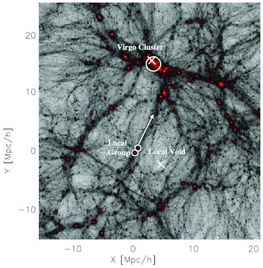
A rendering of the density field in a typical constrained simulation. The position of the observed Virgo cluster and the centre of the Local Void is demarcated by two white X’s. The large white circle shows the position of the simulated Virgo cluster, while the region surrounding the Local Void is also clearly empty. A white arrow shows the direction of the local filament as determined by the velocity-shear tensor analysis of the reconstructed local Universe in Libeskind et al. (2015). The filament direction is not perfectly aligned with the direction towards the Virgo cluster. The observed and simulated LG both reside at the super galactic origin, denoted by the two small white circles.
3.2.2 Intermediate and high-resolution hydro runs
Once the low-resolution DM only ICs have been run, their z = 0 snapshot analysed and the cosmographically successful simulations identified, the ICs are regenerated with a higher resolution of 40963 effective particles in a 7.4 Mpc (5 Mpch−1) sphere around the centre of the LG. Small-scale power is added randomly by sampling the ΛCDM power spectrum at the appropriate scales. These ICs are then run with full MHD and galaxy formation (see Section 2.2). Gas cells are added by splitting each DM particle into a DM – gas cell pair with a mass determined by the cosmic baryon fraction. The pair is separated by a distance equal to half the mean inter-particle separation. The centre of mass and its velocity is left unchanged.
The mass and spatial resolution achieved is |$m_{\rm dm}= 1.2\times 10^{6}\, {\rm M}_{\odot }$|, |$m_{\rm gas}= 1.8\times 10^{5}\, {\rm M}_{\odot }$|, and ϵ = 340 pc. At z = 0, the region uncontaminated by lower-resolution elements is a spherical blob roughly 6 Mpc (4 Mpch−1) in radius that includes the LG and hundreds of field and satellite dwarf galaxies. These simulations represent the intermediate resolution, constrained LG simulations. The properties of the LG members can be found below in Table 1. They constitute the bulk of the simulations analysed and studied in this paper.
After MHD simulation, the baryonic components of the simulated LGs are examined and subject to additional non-cosmographic criteria, so as to ensure that the simulated galaxies are fair representations of the observed LG. They are visually inspected to ensure they are disky and not bulge dominated.
In order to go to even higher resolution, only three ICs are selected (owing to the high computational cost). These are named 09_18, 17_11, and 37_11: the first number refers to the seed for the long waves, while the second refers to the seed for the short waves. Two overlapping 3.7 Mpc (2.5 Mpch−1) spheres are drawn around the two main z = 0 LG members and are then populated with 81923 effective particles. The mass and spatial resolution achieved is |$m_{\rm dm}= 1.5\times 10^{5}\, {\rm M}_{\odot }$|, |$m_{\rm gas}= 2.2\times 10^{4}\, {\rm M}_{\odot }$|, and ϵ = 220 pc. Note that there are some slight, expected, more-or-less negligible changes to the LG set-up at z = 0, when run with hydrodynamics at 81923 resolution compared with 40963 resolution (see Table 1).
Figs 2 and 3 show face and edge on views of the galactic discs produced by these simulations. The orientations are selected according to the eigenvectors of the moment of inertia tensor computed from the stars within 10 per cent of the virial radius. Fig. 2 shows a mock HST image of the stellar component. Such an image is generated by superimposing U-, V-, and B-band luminosities to the red, green, and blue colour channels, respectively (see Khalatyan et al. 2008). Photometric properties for each star particle can be derived by using stellar population synthesis models to estimate the luminosity in a series of broad-bands. Luminosities for U, V, B, K, g, r, i, and z bands from the Bruzual & Charlot (2003) are tabulated. The effects of dust attenuation are not included.5
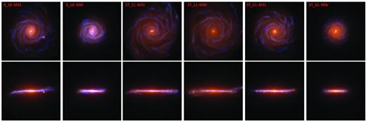
Face on (top) and edge on (bottom) mock HST images of the six highest resolution hestia LG members. The scale of the box is 30 kpc across.
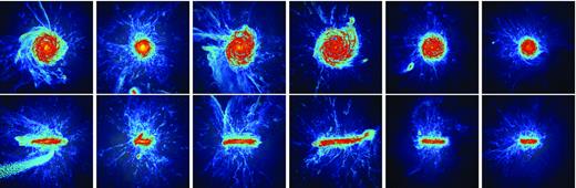
Same as Fig. 2 but showing the gas density. Red indicates higher gas density, blue-black indicates lower density. The scale of the box is 50 kpc across, highlighting the nearby circum-galactic medium.
Fig. 3 shows gas density on a slightly enlarged scale, chosen to highlight circum-galactic gas. Note that, although there are variations in size, mass, bar, etc., most of the hestia LG galaxy members look similar: they are disky spiral galaxies whose halo and stellar mass is within the observed range. See the following sections for a quantification of properties. Fig. 4 is a zoom out and shows one of the high-resolution hestia LGs, including the DM, gas density, and density-weighted temperature. The thermodynamic interaction between galactic, circum-galactic, and inter-galactic LG gas can be seen here.
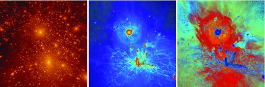
One (17_11) of the high-resolution hestiaz = 0 LGs. The panels show from left to right the DM density (white: high density, red-black: low density), gas density (yellow-white: high density, blue-black low density), and density-weighted gas temperature (yellow-red: 106 K hot gas, dark blue: 104 K cold gas). The two main galaxies are clearly seen as is a smattering of accompanying dwarf galaxies and circum-galactic gas. Panels are all centred on the LG and are 3 Mpc across.
4 RESULTS
The presentation of the results is split into two parts: first a description of the properties of the two main simulated LGs members in comparison to the observed values is presented. The subsequent section focuses on a description of the satellite dwarf galaxies in the simulated LG. This pedagogy is motivated by a qualitative and quantitative comparison with the observed LG. Namely our comparison is limited to properties of the LG where there is good reliable observational data. Characteristics that cannot be directly compared with observations are omitted.
4.1 A description of the main hestia LG members
4.1.1 Local Group dynamics and mass accretion history
Before a description of how the simulated LGs compare to the observed LG in terms of their internal (namely baryonic) properties is shown, in the following section their bulk features – dynamics and mass – are presented together with those of the observed LG. It must be emphasized that the LGs in this work have been ‘bred’ to have certain properties consistent with observations – they have been constructed and selected so as to be accurate representations of the observed LG.
Fig. 5 focuses on the dynamics of the pair, showing how the relative radial and tangential velocities and pair separation are related and compared with the observed values. Note that although hestia LGs are not able to perfectly (within the errors) match simultaneously the radial velocity, the tangential velocity, and the separation as observed in the LG, they are fairly close representations. Recall that by construction they must have separations of 500–1200 kpc and negative radial velocities (no requirement is made of the tangential velocity). For example, the systems shown here, have relative radial velocities of <−100 kms−1 and have tangential velocities of ∼150 kms−1 which is greater than the observed value of ∼20−70 kms−1 from proper motions (van der Marel & Guhathakurta 2008; van der Marel et al. 2012; Fritz et al. 2018), although in agreement with the more controversial value of ∼127 kms−1 from satellite orbital modelling (Salomon et al. 2016). Similarly, most of the systems that have radial velocities consistent with the data (∼−110 kms−1), have separations of <700 kpc, slightly smaller than the observed value of 785 kpc. The total relative velocity (defined as the square root of the sum of the squares of the tangential and radial velocities) and separation is, however, consistent with that of the LGs.
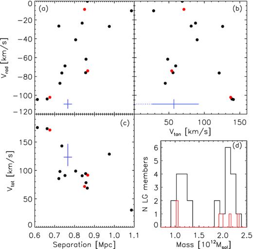
The dynamics of simulated LGs. (a) The relative radial velocity versus pair separation. (b) Radial versus tangential velocity. (c) The total relative velocity versus pair separation. (d) The mass function for all LG members. The black dots/line refer to LGs simulated at the intermediate resolution while the red dots/line are for the high resolution. In blue, we show the observational values with error bars. Solid blue line is vtan = 57 ± 30 kms−1 from Gaia proper motions (van der Marel et al. 2019), while dotted line is vtan < 34 kms−1 from HST proper motions (van der Marel et al. 2012).
The mass accretion history of the hestia LGs is shown in Fig. 6 and computed by linking the most massive progenitors between snapshots (see Section 3.1). The mass accretion histories of the six high-resolution LG members are shown as individual red and green curves (for M31 and MW, respectively), while the mass accretion histories of the 26 intermediate resolution LG galaxies are quantified in terms of their median and 2σ spread. The mass accretion histories are compared with an empirical curve suggested by McBride, Fakhouri & Ma (2009) obtained by averaging over the accretion history of many dark matter haloes with masses similar to the MW drawn from a large cosmological simulation without environment consideration. Although this is not an observed quantity, it is included here to highlight a key difference between the haloes in our (constrained) simulations and those found in unconstrained simulations of the same mass. The empirical McBride et al. (2009) fit allows us to compare if there are any systematic differences introduced by the combination of constrained ICs and selection criteria. Indeed this is the case: hestia LGs grow slower or at the same rate as their unconstrained counterparts at early times (at z ≲ 2). hestia LGs appear to have a ‘growth spurt’ (between 1 ≲ z ≲ 2) where they increase their assembled mass from |$\sim 10\,\,\text{to}\,\,40{{\ \rm per\ cent}}$| such that |$\sim 70\,\,\text{to}\,\,90{{\ \rm per\ cent}}$| of their mass is in place by z ≈ 1. This can also be seen by the redshift at which the haloes have acquired half their z = 0 mass: for unconstrained similarly massed MW/M31 analogues this occurs, on average, at z = 1.1. While for hestia LGs this occurs, on average, at z = 1.4 roughly one billion years earlier. Specifically, only a fifth of hestia MW/M31 members assemble half their mass later than average unconstrained similarly massed halo. Note that a few of the Auriga haloes show similar growth spurts (Fattahi et al. 2019), although these are not controlled for cosmographic environment. Also, although not shown here, the median mass accretion history of the Auriga suite is coincident with the McBride et al. (2009) curve for z < 1 and roughly follows it for z > 2, suggesting that the mass accretion history of the hestia simulations is directly influenced by the constrained nature of the environment.
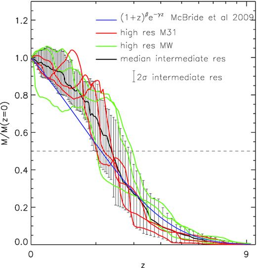
The mass accretion history of the largest progenitor halo of the two main LG haloes. The growth history of each z = 0 LG halo is computed via a merger tree described in Section 3.1. The intermediate and high-resolution runs are indicated by the black and red lines, respectively. In blue, an empirical relation obtained by McBride et al. (2009) by averaging over many MW/M31 mass haloes drawn from a large cosmological simulation is shown. For the most part, hestia LGs grow slower or at the same rate as their unconstrained counterparts at early times (say at z > 2) but then have a growth spurt (at around 1 < z < 2) that results in them having already assembled the bulk of their mass before their unconstrained analogues.
An inspection of the mass accretion history of Fig. 6 highlights the salient point that to have morphologically similar galaxies to the observed LG, the mass accretion history must be systematically different from equally massed, but environmentally unconstrained, analogs (e.g. see Naab & Ostriker 2006; Sales et al. 2012). In fact, a systematic deviation of around 1σ between the mean mass accretion history of constrained and unconstrained LGs was found by Carlesi et al. (2020). Note that most simulations of ‘MW-type galaxies’ are not random but require either quiet merger histories or isolation. What is perhaps surprising is that constrained simulations based on measurement of the local velocity field has already been shown to produce significantly and systemically different mass accretion histories for the simulated Virgo cluster (Sorce et al. 2016c, 2019). Here, a similar behaviour is seen on mass scales that are 2 orders of magnitude smaller.
4.1.2 Baryonic components of individual LG galaxies
In this section, the baryonic component of the simulated LG members is examined. Fig. 7 presents the Mstar versus Mhalo relation for the simulated LGs, along with the empirical ΛCDM relationship suggested by Guo et al. (2010). Note that the sample sits well within both the permitted range suggested by Guo et al. (2010), as well as the range consistent with observations. It is thus noted that the location of a galaxy–halo pair on such a plot is influenced principally by the Auriga galaxy formation model rather than the constraining nature of the ICs. These simulated LGs are also fully consistent with the upper most value for the mass of the entire LG inferred from the timing argument (from proper motion measurements of M31 by van der Marel et al. 2012, see also McLeod et al. 2017). Note however, that due to the still small number of realizations a continuous distribution of halo masses is not produced, specifically lacking haloes with |$M_{\rm halo}\approx 1.25\!-\!1.9 \times 10^{12}\, \mathrm{M}_{\odot }$|, which would be the median of the observationally permitted limits. This shortcoming is entirely due to the (relatively) low number of LGs produced and examined here, and not to a physically meaningful reason. (This gap is also visible in Fig. 5d.)
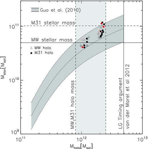
The Mstar versus Mhalo relation for the hestia LGs. Plotted in black is each galaxy at the intermediate (40963) resolution while in red is the high (81923) resolution. In dark grey, we plot the Mstar−Mhalo relation suggested by Guo et al. (2010). Also included are constraints on the MW and M31 dark halo and stellar mass (see Table 1), as well as the total LG mass from the timing argument, based on measurements of M31’s proper motion (van der Marel et al. 2012).
The individual LG galaxies simulated here have circular velocity profiles that match well the observational data. Specific features of a galaxy’s circular velocity profile – a steep rise in the inner parts (within ∼ kpc) followed by a flattening in the outer parts, are generic features of how disc galaxies form in this model of the ΛCDM paradigm. Fig. 8 shows the circular velocity profiles computed from the mass distribution namely |$v_{\rm circ}(r)=\sqrt{2GM(\lt r)/r}$|, where M is stellar mass, gas mass, dark matter mass, or total mass. The observations of MW’s and M31’s circular velocity published by Huang et al. (2016) and Chemin, Carignan & Foster (2009), respectively, are shown as well. Indeed all circular velocity profiles show this observed behaviour, and are included as a dynamical sanity check of the kinematics of these galaxies.
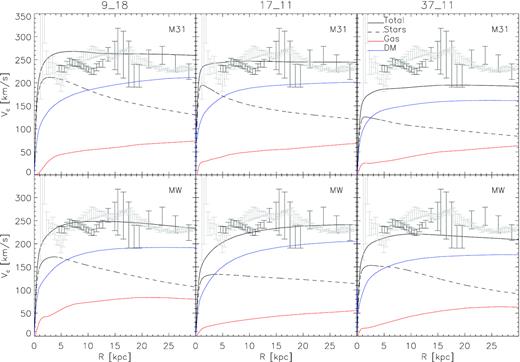
Circular velocity of the high-resolution simulated LGs considered here. The more massive halo (M31 analogue) is plotted in the upper row, while the less massive one (MW analogue) is shown in the bottom row. The total circular velocity is drawn as the black line while the circular velocity for the stellar, gaseous, and dark matter components is shown as dashed black, red, and blue, respectively. Observational values for the MW from Huang et al. (2016) and for M31 from Chemin et al. (2009) are shown as the black and grey error bars, respectively. Note that within 30 kpc, |$V_{\rm c}^{\rm MW}\lt V_{\rm c}^{\rm M31}$|, consistent with the higher stellar mass shown in Table 1.
4.1.3 Morphology of LG galaxies
The stellar component of the simulated LG can be decomposed into a bulge and disc component by fitting an exponential disc and bulge to the estimated surface brightness profile. Accordingly, an effective bulge radius (Reff) and disc scale length (Rdisc) can be inferred. Note that this is different from a dynamical bulge–disc decomposition often employed in numerical simulations. The reason this dynamical measure is avoided here is because observationally such decompositions are unobtainable, while surface brightness modelling can be performed on both the MW (e.g. see Bland-Hawthorn & Gerhard 2016, for a review) and on M31 (Courteau et al. 2011) amongst other galaxies.
Fig. 9 shows the stellar surface density profile of the simulated LG galaxies, as seen from a face-on projection. The method presented in Sparre & Springel (2017) is employed wherein the contribution of a bulge and disc component is modelled with a Sérsic and an exponential profile, respectively. The best-fitting parameters have been obtained in a simultaneous fit of the disc and bulge. Only stars within 0.15R200 are included in the fit to avoid a contaminating contribution from halo stars. The fitting parameters are presented in Table 2 along with the estimated mass belonging to the bulge and disc (D/T).
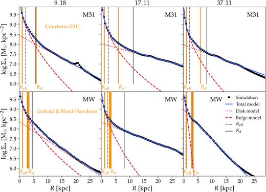
The surface brightness profile of the simulated LG galaxies (M31 top row, MW bottom row) is modelled by the sum of a Sérsic profile describing the bulge (dashed red line) and an exponentially decaying disc (dotted red line). The total model is shown by the blue curve, while the simulation’s values are black dots. The bulge effective radius (Reff) and the disc scale length (Rd) for the simulation are shown with dashed and solid grey vertical lines, while the observed values for M31 and the MW are shown in orange (with the width of the bands indicating the observational error). See Table 2.
Structural parameters for the high resolution M31 and MW. The columns show galaxy simulation ID, effective radius of the Sérsic profile describing the bulge (in kpc) for M31 and MW, the disc scale length (in kpc) for M31 and the MW, the Sérsic index for M31 and MW, and the disc-to-total mass fraction for M31 and MW. References: [1] Courteau et al. (2011); [2] Gerhard & Bland-Hawthorn (private communication); [3] Bland-Hawthorn & Gerhard (2016).
| ID | |$R^{\rm M31}_\text{eff}$| | |$R^{\rm MW}_\text{eff}$| | |$R^{\rm M31}_\text{d}$| | |$R^{\rm MW}_\text{d}$| | nM31 | nMW | D/TM31 | D/TMW |
|---|---|---|---|---|---|---|---|---|
| (kpc) | (kpc) | (kpc) | (kpc) | |||||
| 9_18 | 2.11 | 2.88 | 5.64 | 4.50 | 1.81 | 1.80 | 0.46 | 0.38 |
| 17_11 | 2.32 | 1.95 | 11.21 | 7.97 | 2.28 | 1.64 | 0.64 | 0.82 |
| 37_11 | 1.99 | 0.71 | 8.13 | 2.93 | 1.87 | 1.81 | 0.72 | 0.88 |
| Observations | 1.0 ± 0.2 | ∼1 | 5.3 ± 0.5 | 2.5 ± 0.5 | 2.2 ± 0.3 | – | – | – |
| References | [1] | [2] | [1] | [3] | [1] |
Although a robust disc–bulge decomposition of the Galaxy is complicated by our location within it as well as the overlap of these two components, estimates can be made. The situation for M31 is easier, given our observational vantage point. Two salient points may be inferred from Fig. 9: the LG members in these constrained simulation have fairly well-defined bulge and disc components and these are not inconsistent with the published observational values. In some cases, for example the simulated M31 in simulation 09_18, the values are very close to the observations. Similarly the values for the MW in simulation 37_11 are in good agreement with the observations. The conclusions one may draw from such a finding is that even by this specific, highly non-linear metric, the simulations presented here resemble the true LG morphologically.
4.2 A description of the simulated LG dwarfs
The simulations presented here allow for the study of both LG satellites galaxies, as well as the ‘field dwarfs’ in the LG. Only the former are shown here, leaving a description of the field dwarfs to further study. This is because satellite dwarfs can be easily defined (namely substructures within a virial radius) while a complete sample of field dwarfs of the LG is not as straightforward. This is further complicated by the complex (and individual) topology of the resimulated high resolution region.
4.2.1 Mass and luminosity function of satellite dwarfs
One of the most basic tests of any theoretical model that attempts to reproduce the LG, is its prediction of the distribution of satellite galaxy mass. Only substructures that are well resolved with more than 100 star particles and within 250 kpc are shown here. Fig. 10 shows such simulated stellar mass functions. Each of the six high-resolution LG members are shown individually in red and green (for M31 and MW, respectively), while stellar mass functions for the intermediate resolution are grouped together and their 2σ spread is shown. The width of this spread indicates that there is considerable variance in the satellite mass functions: the most massive satellite in one LG has a mass of a mere few |$10^{7}\, \mathrm{M}_{\odot }$|, while in others the most massive satellite can be up to three orders of magnitude larger. In the highest resolution runs a difference in the number of satellites (most likely owing to the factor of ∼2 differences in LG masses) is seen: in one case there are more than 50 satellites (more massive than |$M_{\star }\gt 10^{4}\, \mathrm{M}_{\odot }$|) in another just 15.
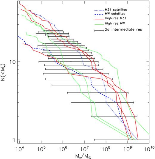
The stellar mass function of satellite galaxies in the hestia runs. The intermediate resolution simulations are shown as 2σ spreads in black, while the high-resolution simulations are shown individually in red and green. In blue dotted and dashed lines, we show the observed stellar mass function for the satellites of M31 and the MW, respectively. For the observed data, stellar masses have been inferred by applying Woo, Courteau & Dekel (2008) mass-to-light ratios to the luminosities published in McConnachie (2012). Note that the observations are likely to be incomplete below |$M_{\star } \lt 10^{5} \, \mathrm{M}_{\odot }$|.
The luminosity function of satellites in the simulated LGs are shown in Fig. 11. The picture is similar to the stellar mass function namely a wide spread for the simulated LGs that straddle some of the observed data. The luminosity function is well matched to the MW’s satellite luminosity function over many orders of magnitude, but shows an under prediction with respect to M31 below LV ∼ 107 L⊙. The reader is reminded that the data is only believed to be complete above LV ≳ 105 L⊙ (e.g. see Yniguez et al. 2014).
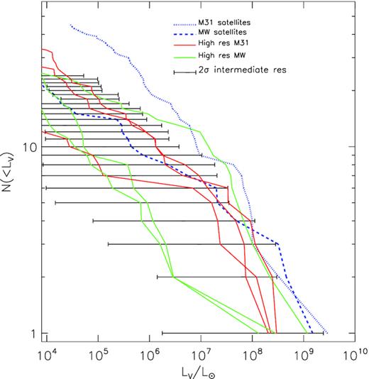
The V-band luminosity function of satellite galaxies in the hestia runs. The intermediate resolution simulations are shown as 2σ spreads in black while the high-resolution simulations are shown individually in red and green. In blue dotted and dashed lines, we show the observed luminosity function for the satellites of M31 and the MW, respectively, from McConnachie (2012). Note that the observations are likely to be incomplete below LV < 105 L⊙.
The variance of the satellite mass and luminosity function originates in the interplay between the randomness of the small scale modes introduced, the way they couple to the larger scale constrained modes, the dwarf merger history and the inherently stochastic nature of galaxy formation at these scales (namely the susceptibility of nascent dwarf galaxies to photoevaporation due to background ionizing radiation, strangulation, various stripping mechanisms, mergers, cold gas accretion, and feedback due to stellar winds, supernovae, and possibly even AGNs).
Regardless of the inherent and expected variance in comparing the satellite stellar mass and luminosity functions to each other and to the data, the simulated LGs straddle the observed data, broadly reproducing the mass and luminosity distribution of satellite dwarfs seen in the LG.
4.2.2 Radial concentrations
In this section, and in Fig. 12, the radial distribution of satellite galaxies is examined and compared with the observed data. In both the simulations as well as the observations, a conservative luminosity cut is made at LV > 105L⊙. Such a plot indicates how centrally concentrated or spatially extended satellite distributions around their host haloes are. Similar to the satellite mass functions presented in the preceding section, there is a large variance for this measure. However the radial concentrations of the two LG members (data compiled by Yniguez et al. 2014, and updated with the dwarfs discovered since then) are themselves significantly different. In the MW case at least, this may partly be explained by the difficulty in detecting satellites at low galactic latitude due to obscuration by the MW’s disc (i.e. the Zone of Avoidance). On the other hand, the distance to known MW satellites are known to better accuracy than for M31, hence the smaller error corridors.
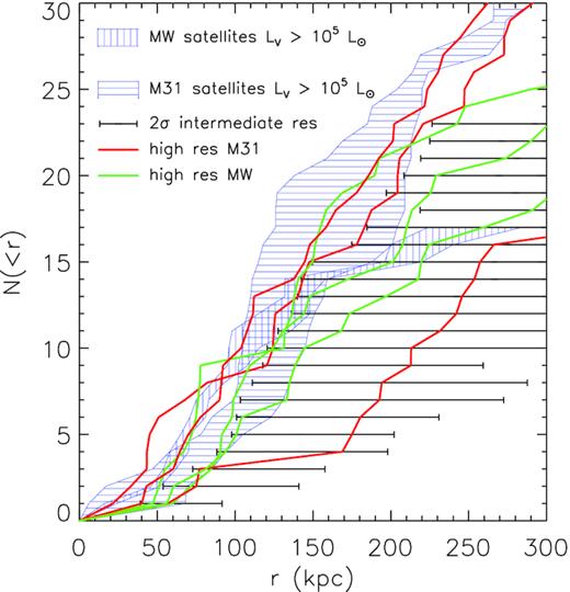
The radial distribution of satellite galaxies whose luminosity LV > 105 L⊙. This cut is chosen since it is believed to be the completeness limit for the observed LG satellites. Data for the M31 and MW are shown as the blue horizontally and vertically hatched (respectively) corridors. Observational data is taken from the compilation presented in Yniguez et al. (2014) updated with newly discovered dwarfs.
Different hestia simulation runs have different levels of satellite concentration. In general these simulations have fewer satellites in the central regions than observed. This is, at least in part, likely a resolution effect; as the density in the inner regions of the halo increases (especially due to the presence of a dense baryonic disc), it becomes harder and harder to identify subhaloes as over densities against the background. Considering also the physical processes whereby subhaloes are destroyed (e.g. Richings et al. 2020), the paucity of satellites inhabiting the inner regions, can be understood (for a detailed description of this see Onions et al. 2012). The following conclusions may be drawn from Fig. 12: a single hestia run follows the M31 satellite radial distribution within the errors out to 250 kpc. This in and of itself is a remarkable success. A number of other runs match the M31 data out to ∼200 kpc. One run matches the MW data from around 40 to 100 kpc. Most of these simulations are not as concentrated as the observations, but the large variety in radial concentrations and the fact that in a few cases the observations are matched, speaks to the reproducibility of this quantity. We note that Samuel et al. (2020) conducted a thorough study of the radial concentrations of simulated MW mass haloes that are found both in isolation and in pairs. The results presented here are consistent with that work, as both show large variations in the radial distribution of satellites within 300 kpc of the host. It is thus unlikely that environment plays a critical role in the satellite radial distribution.
4.2.3 The presence of a Magellanic Cloud or M33 analogue
The last near-field cosmographic feature examined and compared here is the presence of a Magellanic Cloud or M33-like object. The frequency of a Magellanic cloud like object has been studied in a number of papers (see e.g. Boylan-Kolchin, Besla & Hernquist 2011a; Busha et al. 2011, among others). In fact there is a striking agreement between the frequency with which observational and theoretical studies have found Magellanic-type systems around MW-type galaxies. For example Liu et al. (2011) find that less than ∼10 per cent of isolated MW mass galaxies host such systems in the SDSS, while Boylan-Kolchin et al. (2010) find the same frequency in large cosmological simulations. Pre-Gaia estimates of the Magellanic cloud mass are around |$10^{10}\, \mathrm{M}_{\odot }$| (van der Marel & Kallivayalil 2014) while some of the more modern estimates put it at roughly an order of magnitude higher or close to 1/10th of the MW halo mass (Erkal et al. 2019). Not as much work has been done on identifying M33 type galaxies near M31 type hosts. However detailed studies attempting to study M33 like objects in zoom simulations have been carried out by, for example, Mostoghiu et al. (2018) in a bid to understand its formation. M33 is roughly the same mass as the LMC but much further away from M31 than the LMC is from the MW (230 versus 55 kpc).
Fig. 13 shows the mass of satellites as a function of the distance from their host in the form of a ‘heat map’, namely the darker a region is in this figure the more subhaloes have a given distance and mass.. The most massive satellite per host is shown as a circle. Some 73 per cent of the LG members presented here have subhaloes more massive than the lower pre-Gaia estimate, while only one (|$\sim 4{{\ \rm per\ cent}}$|) has an object consistent with the higher mass estimate. A few of these are at the distance of the observed Magellanic system, namely 55 kpc. In fact as can be gleaned from Fig. 13, there are two systems that one could liberally call ‘Magellanic cloud analogues’. Similar conclusions can be made regarding an M33 analogue: some massive satellites are found at distances of around 230 kpc although these are generally not as massive as the |$1.6\times 10^{11}\, {\rm M}_{\odot }$| suggested by Shaya & Tully (2013).
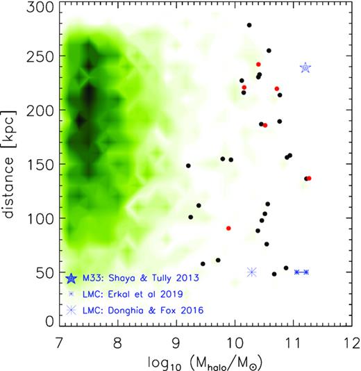
The mass of hestia satellites plotted against the distance from their host centre is shown here as a heat map with black regions denoting more satellites and white regions denoting no satellites. In black and red, we show the most massive satellite in each the intermediate and high resolution run, respectively – namely a Magellanic cloud or M33 analogue. The blue asterisks denote two observational LMC data points: the small connected ones are from employing data from Erkal et al. (2019) Gaia DR2 and the large one is from the seminal review of D’Onghia & Fox (2016). The blue star is the observational data for M33 from Shaya & Tully (2013).
This is not a deficit in our ability to model the Magellanic or M33 systems. The reader is reminded that structures on these scales are entirely unconstrained and thus their frequency should not a priori be any different from an unconstrained simulation of an MW mass halo. On the other hand, given that these simulations force a specific cosmographic matter distribution (namely an LG), the presence of a Magellanic cloud like object is likely to be different compared with other non-LG like environments. Thus in some cases, the LGs shown here are able to produce Magellanic Cloud or M33 like analogues.
5 SUMMARY AND DISCUSSION
The properties of galaxies are known to be influenced by their environment (e.g. Dressler 1980). This is because the most basic characteristics according to which galaxies are described (such as star formation rate, merger history, colour, morphology, angular momentum, baryon fraction, mass, etc.) are not only inter-dependent, but are determined, to an extent, via environmental controls (Courtois et al. 2015; Sorce, Creasey & Libeskind 2016b). For example, galaxies without a large supply of cold gas (or where the gas supply is inhibited from cooling) will not be efficient at forming stars (Barnes & Hernquist 1991). Galaxies in dense environments are likely to experience more active merger histories (Jian, Lin & Chiueh 2012) and thus are less likely to be rotationally supported discs. On the other hand, the current paradigm of structure and galaxy formation (namely the ΛCDM model combined with what is known theoretically and empirically about how galaxies form) has succeeded immensely when describing the large-scale properties of the galaxy distribution. Statistical properties such as n-point correlations functions, galaxy bimodality, or the density–morphology relationship have been understood. No existential challenges to the ΛCDM paradigm remain on large scales or when scrutinising the statistical properties of the galaxy population.
Yet challenges have been found on small scales, specifically on scales of dwarf galaxies (|$\sim 10^{9}\, \mathrm{M}_{\odot }$|) and below (Bullock & Boylan-Kolchin 2017). Some authors have even referred to these challenges collectively as the ‘small-scale crisis of ΛCDM’. Yet what is often overlooked is that in this regime – where the smallest dwarf galaxies are examined, the only reliable data is local data, within our patch of the local Universe. The reason for this is simple: small faint, low surface brightness, low-mass galaxies are only observable in our vicinity. Given that galaxy environment is known to play a role in galaxy formation, it follows that simulations that attempt to explain challenges in this regime ought to examine the ‘correct’ environment.
This cogent methodology is not lost on the community at large. Most studies that attempt to explain small scale phenomena do so by examining dwarfs in MW mass haloes. Some studies, such as the ELVIS (Garrison-Kimmel et al. 2014) or the APOSTLE (Fattahi et al. 2016; Sawala et al. 2016b) simulations, go further and model the binarity of the LG, namely the existence of a second MW mass halo (i.e. the Andromeda system) around an Mpc away. None of these studies explicitly control for the environment on quasi linear or linear scales – namely the existence of the Virgo cluster, the local void and the local filament, cosmographic features that individualize our local environment and regulate critical aspects of galaxy formation: merger history (Carlesi et al. 2020), halo growth (Sorce et al. 2016c), gas supply, and bulk motion (Hoffman et al. 2015). Indeed, a comprehensive approach describing how the local cosmic web regulates galaxy formation, was put forward by Aragon Calvo, Neyrinck & Silk (2019) who examined in general detail how the cosmic web imprints itself on galaxy properties.
The issue at stake here is of a Copernican nature. To what extent the LG is fair representative of objects of its kind, and thereby to what extent its observed properties represent LG-like objects at large. This where constrained simulations of the LG are making the difference – by controlling both the actual local environment and by experimenting with the physics of galaxy formation, on the computer.
It is within this context that we have embarked on the hestia project – High resolution Environmental Simulations of The Immediate Area. Accordingly, the CosmicFlows-2 catalogue (Tully et al. 2013) of around 8000 peculiar velocities is employed to characterize the local cosmography. ICs are then generated which are constrained to reproduce the z = 0 large-scale structure, namely the gravitational attractors and repellers that constitute voids and cluster in the local Universe. Non-linear phenomena – such as the existence of a galaxy pair at the correct location with respect to the local cosmography – are not constrained but are reproduced through trial and error at low resolution but are more likely to be found in constrained simulations than in random simulations (Hoffman et al. 2015). The ICs are run with the cosmological MHD code arepo (Springel 2010) and the Auriga galaxy formation model of Grand et al. (2017).
The result of the procedure is a set of 13 intermediate and 3 high-resolution cosmological magneto-hydrodynamical simulation of the LG within the dynamical environment as described by measurements of the peculiar velocity field. The Virgo cluster is reproduced in the correct location and at the correct distance as is a void region analogous to the Local Void. A filamentary structure, abutted by the simulated Local Void and stretched from the LG to the Virgo cluster is also reproduced. Within this environment, pairs of galaxies are found at roughly the correct distance from each other and from Virgo, with roughly the correct mass and mass ratio, negative relative velocity, and with cold gas discs. The simulated rotation curves of the LG analogues are in rough agreement with the observations. Dwarf galaxies, as well as galactic disc features (such as bars, spiral arms, etc.) are resolved. The satellite galaxies have similar stellar mass distributions and radial concentration as observed. The hestia runs also produce large Magellanic cloud and M33-like objects.
The present hestia simulations successfully reproduce many of the observed features of the local universe on scales ranging from the |$10^{14} \, \mathrm{M}_{\odot }$| Virgo cluster more than 10 Mpc away, the local filament (within which the LG resides) on the scale of a few Mpc, the inter-LG sub-Mpc scale and all the way down to sub-virial scales within the MW and M31 galaxies. The large scales are strongly constrained by the CF2 velocity data and are robustly reproduced by the simulations. Going down to smaller and smaller scales, the constraining power of the data diminishes and the variance within the different realizations increases. The conclusion from this work is that the wide range of LG properties reported here – including the inner structure of the MW and M31, stellar and light distribution, distribution of satellites, environment – is reproduced within the constrained variance. Some of these properties are reproduced by some of the galaxies – not necessarily all of them. This opens the door to further studies on the nature of the LG and its formation. Three immediate routes are to be pursued: the increase of the ensemble of constrained simulations (thereby studying the statistical significance of our results); the increase of resolution (thereby studying the numerical robustness of the results); and experiments with the model of galaxy formation physics. These will enable a better understanding the physics of galaxy formation and to address the Copernican issue regarding our role in the universe. This work will be extended along these routes.
ACKNOWLEDGEMENTS
NIL acknowledges financial support of the Project IDEXLYON at the University of Lyon under the Investments for the Future Program (ANR-16-IDEX-0005). NIL and PW acknowledge support from the joint Sino-German DFG research Project ‘The Cosmic Web and its impact on galaxy formation and alignment’ (DFG-LI 2015/5-1). NIL, MSP, and PW thank the DAAD for PPP grant 57512596 funded by the BMBF. CP acknowledges support by the European Research Council under ERC-CoG grant CRAGSMAN-646955. YH has been partially supported by the Israel Science Foundation grant ISF 1358/18. HMC acknowledges support from the Institut Universitaire de France and the CNES. AK and GY are supported by MICIU /FEDER (Spain) under research grant PGC2018-094975-C21. AK further acknowledges support from the Spanish Red Consolider MultiDark FPA2017-90566-tREDC and thanks Wire for 154. ET was supported by ETAg grant IUT40-2 and by EU through the ERDF CoE TK133 and MOBTP86. SP is supported by the program ‘LPI new scientific groups’ N01-2018. MV acknowledges support through an MIT RSC award, a Kavli Research Investment Fund, NASA ATP grant NNX17AG29G, and NSF grants AST-1814053, AST-1814259, and AST-1909831. The authors gratefully acknowledge the Gauss Centre for Supercomputing e.V. (www.gauss-centre.eu) for funding this project by providing computing time on the GCS Supercomputer SuperMUC at Leibniz Supercomputing Centre (www.lrz.de). The authors also acknowledge Joss Bland-Hawthorn and Ortwin Gerhard for their help in quantifying the structural parameters of the Galaxy. Azadeh Fattahi is also acknowledged for her help in providing some of the observational LG data.
DATA AVAILABILITY
The data underlying this article will be shared on reasonable request to the corresponding author.
Footnotes
ahf is publicly available from http://popia.ft.uam.es/AHF/Download.html
Note that the method for computing luminosities for the purpose of the mock HST images is not identical to what is used in Fig. 11, described in Section 3.1. Despite the difference in method, the results are nearly identical. The differences arise from the use of different pre-existing codes for the purpose of computing luminosities of star particles.
