


ABSTRACT
The Discrete Element Method (DEM) is frequently used to model complex granular systems and to augment the knowledge that we obtain through theory, experimentation, and real-world observations. Numerical simulations are a particularly powerful tool for studying the regolith-covered surfaces of asteroids, comets, and small moons, where reduced-gravity environments produce ill-defined flow behaviours. In this work, we present a method for validating soft-sphere DEM codes for both terrestrial and small-body granular environments. The open-source code chrono is modified and evaluated first with a series of simple two-body-collision tests, and then, with a set of piling and tumbler tests. In the piling tests, we vary the coefficient of rolling friction to calibrate the simulations against experiments with 1 mm glass beads. Then, we use the friction coefficient to model the flow of 1 mm glass beads in a rotating drum, using a drum configuration from a previous experimental study. We measure the dynamic angle of repose, the flowing layer thickness, and the flowing layer velocity for tests with different particle sizes, contact force models, coefficients of rolling friction, cohesion levels, drum rotation speeds, and gravity levels. The tests show that the same flow patterns can be observed at the Earth and reduced-gravity levels if the drum rotation speed and the gravity level are set according to the dimensionless parameter known as the Froude number. chrono is successfully validated against known flow behaviours at different gravity and cohesion levels, and will be used to study small-body regolith dynamics in future works.
1 INTRODUCTION
Past and ongoing space missions like NEAR, Dawn, Hayabusa, Rosetta, Hayabusa2, and OSIRIS-REx have provided us with a glimpse into the diverse features found on small-body surfaces (Cheng et al. 1997; Fujiwara et al. 2006; Glassmeier et al. 2007; Russell et al. 2007; Lauretta et al. 2017; Watanabe et al. 2019). Images show that asteroids are covered with a layer of boulders and regolith, where surface grains vary drastically in terms of size, shape, and material composition (Murdoch et al. 2015). Fundamentally, particles interact with one another the same on small bodies as they do on the Earth. If an external event agitates a system, grains collide and dissipate energy according to the same contact laws, where their resulting motion depends on collision velocities, internal friction, shape, and material. However, cohesive and electrostatic forces are expected to be more influential in reduced-gravity environments than they are on the Earth (Scheeres et al. 2010), and we are still trying to understand the implications for bulk regolith behaviour.
A limited number of missions have conducted extensive, in-situ operations on small-body surfaces. In 2014, the European Space Agency deployed the Philae lander to the surface of comet 67P/Churyumov-Gerasimenko as part of the Rosetta mission (Glassmeier et al. 2007). After its landing system failed, Philae rebounded several times on the surface. The lander’s bouncing behaviour has since been used to characterize the surface mechanical properties of the comet (Biele et al. 2015). More recently, the German, French, and Japanese space agencies (DLR, CNES, and JAXA) delivered several hopping rovers to the surface of the asteroid Ryugu during the Hayabusa2 mission. Data from the rovers and spacecraft are being used to interpret Ryugu’s material and geological properties (Jaumann et al. 2019; Sugita et al. 2019). While enlightening, in-situ data are sparse, and additional information is required to explain the phenomena shown in lander and spacecraft images.
The need to improve our understanding of regolith dynamics in reduced-gravity environments is also important for several upcoming missions. For instance, the Japan Aerospace Exploration Agency’s (JAXA) Martian Moons eXploration (MMX) mission (Kuramoto, Kawakatsu & Fujimoto 2018) will deploy a small rover to the surface of Phobos. The wheeled rover, provided by the Centre National d’Etudes Spatiales (CNES) and the German Aerospace Center (DLR), will operate for three months on Phobos and cover an anticipated distance of several meters to hundreds of meters (Tardivel, Lange & the MMX Rover Team 2019; Ulamec et al. 2020). In addition to providing important information regarding the geological and geophysical evolution of Phobos, an understanding of Phobos’s surface mechanics is critical to the design and operations of the rover itself. Knowledge of regolith dynamics will also be essential for interpreting the consequences of the impact of NASA’s DART mission (Cheng et al. 2017), and for preparing the landing of CubeSats on the surface of the asteroid Didymoon during ESA’s Hera mission (Michel et al. 2018).
Laboratory experiments have been developed to study reduced-gravity impact dynamics (Colwell & Taylor 1999; Murdoch et al. 2017; Brisset et al. 2018), avalanching (Kleinhans et al. 2011; Hofmann, Sierks & Blum 2017), angle of repose (Nakashima et al. 2011), and dust lofting (Hartzell et al. 2013; Wang et al. 2016). These tests are difficult and costly to run however, as they often rely on parabolic flights, drop-tower set-ups, or shuttle missions to reach variable gravity conditions. As a result, numerical modelling has become an essential tool for studying planetary surfaces. Tests can be carried out across large parameter spaces, and flow behaviours can be analysed in impressive detail. For example, numerical models have been used to study the strength, re-shaping, and creep stability of rubble-pile asteroids (Sánchez & Scheeres 2012, 2014; Yu et al. 2014; Zhang et al. 2017). The code pkdgrav (Richardson et al. 2000; Stadel 2001) was used to investigate lander–regolith interactions within the context of the Hayabusa2 mission (Maurel et al. 2018; Thuillet et al. 2018), and the code esys-particle was used to simulate particle segregation on asteroid surfaces (Tancredi et al. 2012).
Codes pkdgrav and esys-particle and the code by Sànchez and Scheeres simulate granular systems using the Discrete Element Method (DEM). In DEM, surfaces are modelled at the grain level, where various contact laws are used to calculate the kinematics resulting from inter-particle collisions. It is imperative that these models are correctly implemented in the code in order for it to produce reliable results. As such, the goal of this work is to present a robust framework for validating granular DEM codes. The open-source code chrono is subject to extensive benchmark testing, and is introduced as a strong platform for future use in the planetary science community. In these current code developments, we neglect electrostatic and self-gravity forces, and focus on the effects of rolling resistance, cohesion, and gravity level. We validate the code by comparing simulations against existing experimental and numerical studies, and by analysing the flow behaviour in a rotating drum in detail. Tumbler experiments have been conducted at increased gravity levels using centrifuges (Brucks et al. 2007) and reduced-gravity levels using parabolic flights (Kleinhans et al. 2011). The centrifuge experiments show that the dynamic angle of repose in the drum collapses on to a single curve when plotted against a non-dimensional parameter known as the Froude number. This observation has been reproduced in DEM simulations when |$g \ge$| 9.81 m s−2 (Richardson et al. 2011), but not when |$g \le$| 9.81 m s−2. We show that the same flow patterns exist when |$g \le$| 9.81 m s−2.
This paper is organized as follows: In Sections 2 and 3, we introduce the open-source code used in this study and explain how the code was modified in order to improve its accuracy for reduced-gravity environments. In Section 4, we present a set of low-level tests to evaluate each aspect of the modified code. Then, in Section 5, we perform a more complex validation study by comparing experimental and numerical results for a ‘sand piling’ test. Finally, in Section 6, we analyse flow behaviour in a rotating drum under reduced-gravity conditions, with varied particle cohesion.
2 CHRONO
The simulations presented in this paper are conducted using an open-source dynamics engine called chrono (Tasora et al. 2016). chrono is used to model either rigid-body or soft-body interactions and can be executed in parallel by using the OpenMP, MPI, or CUDA algorithms for shared, distributed, or GPU computing (Mazhar et al. 2013; Tasora et al. 2016). Past chrono studies have spanned a wide range of applications, including structural stability (Coïsson et al. 2016; Beatini, Royer-Carfagni & Tasora 2017), 3D printing (Mazhar, Osswald & Negrut 2016), terrain–vehicle interactions (Serban et al. 2019), and asteroid aggregation (Ferrari et al. 2017). Given its versatility, users must install the software and construct physical systems based on their individual needs. This study simulates granular systems using the smooth-contact code (SMC) implemented in the chrono::parallel module.
In equations (1) and (2), m, I, |$\boldsymbol{v}$|, and |$\boldsymbol{\omega }$|, respectively, denote the particle mass, rotational inertia, translational velocity, and rotational velocity. |$\boldsymbol{F}_\mathrm{ n}$|, |$\boldsymbol{F}_\mathrm{ c}$|, and |$\boldsymbol{F}_\mathrm{ t}$| are the normal, cohesive, and tangential force components, respectively, |$\boldsymbol{g}$| is the acceleration of gravity, and |$\boldsymbol{T}$| is the torque. |$\boldsymbol{T} = r_\mathrm{ i} \boldsymbol{F}_\mathrm{ t} \times \hat{n}$|, where |$r_\mathrm{ i}$| is the particle radius and |$\hat{n}$| is the unit vector pointing from one particle centre to the other, establishing the contact normal direction (see Fig. 1). The right-hand sides of the equations are summations for all contacts involving particle ‘i’ at the current time, and the equations are applicable to spherical bodies. The specific force and torque models implemented in chrono are discussed in Section 3.
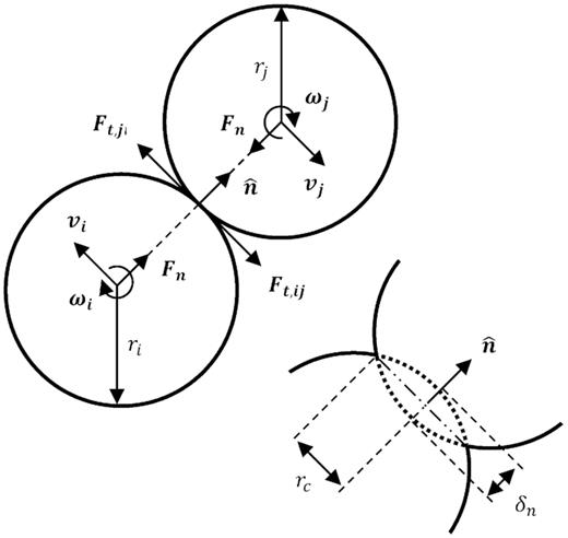
Schematic of the interaction between particles ‘i’ and ‘j’. |$\boldsymbol{F}_\mathrm{ n}$| and |$\boldsymbol{F}_\mathrm{ t}$| are the normal and tangential forces acting on the bodies, respectively, r is the particle radius, |$\boldsymbol{v}$| is the translational velocity, |$\boldsymbol{\omega }$| is the rotational velocity, |$\delta _\mathrm{ n}$| is the particle overlap, |$r_\mathrm{ c}$| is the radial distance of the overlapping area, and |$\hat{n}$| establishes the contact normal direction. Friction moments and cohesion are not depicted.
3 chrono MODIFICATIONS
Adding rolling and spinning friction to granular DEM simulations has been found to significantly improve a code’s ability to replicate bulk granular behaviours like shear strength, dilation response, and shear band development (Iwashita & Oda 1998; Mohamed & Gutierrez 2010). Since the influence of inter-particle friction becomes even more prominent in airless, reduced-gravity environments, it is essential to consider these components when simulating regolith on small-body surfaces. The SMC code in early versions of chrono::parallel (chrono 4.0.0 and earlier) only considers torques induced by sliding friction and tangential displacement. As part of this work, the SMC code in chrono::parallel was updated to incorporate rolling and spinning friction. The code was also modified to include additional force and cohesion models that are relevant for applications in both terrestrial and planetary science. Sections 3.1–3.4 describe the chrono::parallel SMC code in detail, with particular emphasis on the updates available in chrono 5.0.0.
3.1 Normal force models
The advantage of the Flores et al. (2011) force model is that it generates a continuous, repulsive force throughout the entirety of the collision. Adding the Flores et al. (2011) model to the chrono 5.0.0 code release allows us to examine how different force models influence simulation results while preserving the user-defined coefficient of restitution value. Sections 4.1 and 6.4.3 discuss initial observations on the subject, and a detailed comparison will be carried out as part of future work.
3.2 Tangential force models
The tangential contact displacement vector |$\boldsymbol{\delta }_t$| is stored and updated at each time-step. If |$|\boldsymbol{F}_\mathrm{ t}^\prime | \ge |\boldsymbol{F}_{\mathrm{ t,max}}|$|, then |$\boldsymbol{\delta }_\mathrm{ t}$| is scaled to match the tangential force given by the Coulomb friction condition. Fleischmann et al. (2016) describe how |$\boldsymbol{\delta }_\mathrm{ t}$| is calculated, updated, and scaled in more detail.
3.3 Cohesive force models
3.4 Friction models
3.4.1 Rolling friction
3.4.2 Spinning friction
4 TWO-BODY VALIDATION TESTS
DEM codes are often verified against frequently studied problems in granular mechanics, like ‘sand piling’, avalanching, or hopper flow. Specifically, chrono 4.0.0 was checked against a cone penetration experiment, a direct shear experiment, a standard triaxial test, and a hopper flow experiment (Fleischmann et al. 2016; Pazouki et al. 2017). While these validation efforts returned positive results, the simulations compensated for the code’s lack of rolling and spinning resistance by tuning or calibrating the sliding friction parameter to match other experimental results. Large-scale simulations such as these are essential for code validation. However, parameter selection and the bulk behaviour of the system can mask low-level issues with the contact models. For this reason, chrono 5.0.0 was evaluated using seven simple, two-body collision tests before validating the code against more complex systems.
In general, the two-body tests evaluate interactions between two spheres, a box and a plate, or a sphere and a plate. The tests were influenced by previous validation studies (Asmar et al. 2002; Xiang et al. 2009; Ai et al. 2011; Tancredi et al. 2012) and were selected to systematically check each aspect of SSDEM implementation in chrono. When combined, they provide a comprehensive assessment of sliding, rolling, spinning, and collision behaviour. Sections 4.1.1–4.1.7 describe each test and its associated results in more detail.
4.1 Simulations and results
A visual representation of each test presented in this section can be found in Fig. 2, while all simulation parameters are listed in Table 1. If the test involves an interaction between a sphere and a plate or a box and a plate, then the plate is simulated as a large viscoelastic wall with the same material properties as the sphere or box. The simulation time-step is determined using the method described later in Section 5.2 except that the chosen time-step is an order of magnitude smaller than that required by the calculation. A smaller time-step value is applied because the computational cost is negligible. The chrono 5.0.0 code release passes all seven validation tests. Unless otherwise noted, the results do not vary by force model.

Diagram of the seven validation tests presented in Section 4. Bodies on the left depict initial simulation state and bodies on the right illustrate final simulation state. m, g, v, |$\omega$|, |$F_\mathrm{ c}$|, and |$F_\mathrm{ g}$| are, respectively, particle mass, gravity level, translational velocity, rotational velocity, cohesive force, and gravitational force.
Simulation parameters for the normal force test (Test 1), the cohesive force test (Test 2), the normal impact test (Test 3), the oblique impact test (Test 4), the sliding test (Test 5), the rolling test (Test 6), and the spinning test (Test 7).
| Property | Symbol | Test 1 | Test 2 | Test 3 | Test 4 | Test 5 | Test 6 | Test 7 |
|---|---|---|---|---|---|---|---|---|
| Time-step (|$\mu \mathrm{ s}$|) | t | 10 | 10 | 10 | 10 | 10 | 10 | 10 |
| Body diameter (m) | d | 1 | 1 | 1 | 1 | 1 | 1 | 1 |
| Body mass (kg) | m | 1 | 1 | 1 | 1 | 1 | 1 | 1 |
| Young’s modulus (MPa) | E | 0.5 | 0.5 | 0.5 | 0.5 | 0.5 | 0.5 | 0.5 |
| Poisson’s ratio | |$\nu$| | 0.3 | 0.3 | 0.3 | 0.3 | 0.3 | 0.3 | 0.3 |
| Static friction coefficient | |$\mu _\mathrm{ s}$| | 0.3 | 0.3 | 0.3 | 0.3 | 0.5 | 0.3 | 0.3 |
| Dynamic friction coefficient | |$\mu _\mathrm{ k}$| | 0.3 | 0.3 | 0.3 | 0.3 | 0.5 | 0.3 | 0.3 |
| Rolling friction coefficient | |$\mu _\mathrm{ r}$| | 0 | 0 | 0 | 0 | 0 | 0.2 | 0 |
| Spinning friction coefficient | |$\mu _\mathrm{ t}$| | 0 | 0 | 0 | 0 | 0 | 0 | 0.2 |
| Cohesive force (N) | |$F_\mathrm{ c}$| | 0 | 10 | 0 | 0 | 0 | 0 | 0 |
| Gravity level (m s|$^{-2}$|) | g | 9.81 | 8–10 | 0 | 0 | 9.81 | 9.81 | 9.81 |
| Coefficient of restitution | e | 0.3 | 0 | 0–1 | 1 | 0 | 0 | 0 |
4.1.1 Test 1: normal force
The normal force calculation is tested by successively dropping five spheres on to a plate in vertical alignment with one another. Head-on collisions only generate forces in the contact normal direction, so the spheres should not rotate or move laterally when they collide. The test is therefore considered successful if the spheres come to rest in a stacked position on the plate (Asmar et al. 2002). The code passes the test for all three force models.
4.1.2 Test 2: cohesive force
The cohesive force calculation is evaluated by applying an external force to two contacting spheres and verifying that the bodies respond in accordance with their cohesive properties. First, two spheres, ‘i’ and ‘j’, are brought into contact, one on top of the other, with ‘i’ on top of ‘j’, in the absence of gravity. Then, sphere ‘i’ is fixed in space, and gravity is applied to the simulation. The gravitational force acts in opposition to the cohesive force between the bodies and attempts to separate sphere ‘j’ from sphere ‘i’. The test is performed twice: once where the gravitational force is slightly inferior to the cohesive force, and again where the gravitational force equals the cohesive force. The test is considered successful if the spheres remain in contact when |$F_\mathrm{ c} \gt m_\mathrm{ j}g$| but separate when |$F_\mathrm{ c} \le m_\mathrm{ j}g$|. The spheres are expected to separate in the second case due to the elastic nature of the normal force model and the overshoot that occurs when gravity is abruptly turned on. chrono passes the cohesion test. Overshoot and damping behaviour vary by model, as expected (see Fig. 3).
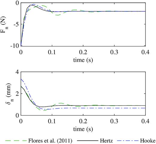
Behaviour of body ‘i’ during the cohesive force test (Test 2), showing the evolution of normal force |$F_\mathrm{ n}$| (top) and particle overlap |$\delta _\mathrm{ n}$| (bottom) for different force models. When a gravitational force of −8 N is applied to two spheres with a 10 N cohesive force, the bodies stabilize at |$F_\mathrm{ n} = -2$| N without separating.
4.1.3 Test 3: normal impact
Based on the implementation of the force models described in Section 3.1, the output coefficient of restitution is expected to match the input value provided by the user. Accordingly, the simulations show that the differences between the expected and measured coefficients of restitution are negligible for the Hooke and Hertz force models. However, the Flores et al. (2011) model is only valid for higher coefficient values (see Fig. 4). The differences between e and |$e^\prime$| when |$e \le 0.8$| are inherent to the model and do not represent issues with the implementation (Flores et al. 2011).
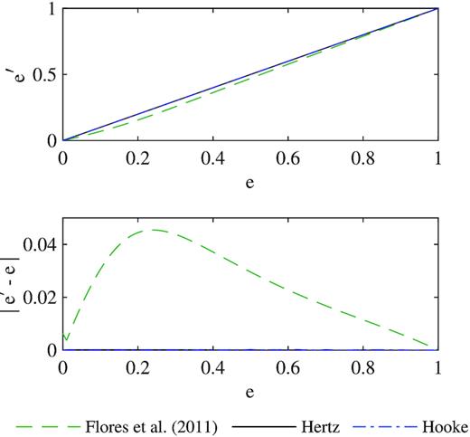
Comparison between the expected and measured coefficients of restitution from the normal impact test (Test 3). The differences between e (the expected COR) and |$e^\prime$| (the measured COR) are negligible for the Hooke and Hertz models but more important for the Flores et al. (2011) model.
4.1.4 Test 4: oblique impact
The test is considered successful if |${\omega }^\prime _{\mathrm{ i}}$| and |$e^\prime _{\mathrm{ t}}$| match theoretical results when |$\phi \ge \phi _{\mathrm{ th}}$|. For example, when |$\mu _\mathrm{ s} = 0.3$| and |$e = 1$|, the threshold impact angle for the full sliding regime is 64.54 deg. When |$\phi _{\mathrm{ th}}$| exceeds 64.53 deg in the simulations, |$\omega ^\prime _{\mathrm{ i}}$| = 3 rad s−1 and |$e^\prime _\mathrm{ t}$| follows equation (25). There are no differences between the measured and theoretical values.
4.1.5 Test 5: sliding
The test is considered successful if the difference between the theoretical and simulated travel distances is less than |$1\times 10^{-3}$| m. If |${v_\mathrm{ o}}$| = 5 m s−1 and |$\mu _\mathrm{ s}$| = 0.5, then the block should slide 2.5484 m before coming to rest. The simulations succeed for these parameters, where the differences between the theoretical and simulated travel distances are |$1 \times 10^{-4}$|, |$3 \times 10^{-4}$|, and |$4 \times 10^{-4}$| m for the Hooke, Hertz, and Flores models, respectively.
4.1.6 Test 6: rolling
Rolling resistance is tested by bringing a sphere into contact with a plane, providing it with an initial horizontal velocity and verifying that it rolls but eventually comes to rest. The torque generated by rolling friction should be constant and non-zero until the sphere stops rotating. The sphere’s position, velocity, and torque profiles should match trends observed in existing works (Zhou et al. 1999; Ai et al. 2011).
In the simulations, the sphere is pushed at an initial velocity of 1 m s−1. Since the sphere is not provided with an initial rotation, it begins by sliding and then starts rolling. Once rolling, the sphere slows down and comes to rest. The rolling resistance torque is constant while the sphere is in motion.
4.1.7 Test 7: spinning
Spinning resistance is tested by bringing a sphere into contact with a plane, providing the sphere with a rotational velocity around the axis normal to the contact plane, and monitoring the sphere’s velocity and torque profiles over time. The test is considered successful if the sphere experiences a constant, non-zero torque while rotating, and if it eventually comes to rest on the plate.
When the sphere is given an initial spin velocity of 1 rad s−1, it comes to a stop as expected. The spinning resistance torque is constant, but slightly lower for the Hooke model than that for the Hertz and Flores models. Since the torque is lower, the sphere takes slightly longer to stop spinning when using the Hooke model. In equation (19), we see that spinning resistance is dependent on both normal force and sphere overlap. The spinning torque varies because |$\delta _\mathrm{ n}$| is different for each force model.
5 PILING TEST
Piling simulations are ideal for demonstrating the importance of rolling resistance in granular DEM studies. In the past, piling tests have been used to compare different rolling friction models in terms of stability and accuracy (Zhou et al. 1999; Ai et al. 2011), to characterize material properties (Zhou et al. 2002; Li, Xu & Thornton 2005), and to benchmark a code’s ability to handle large systems. In this section, we compare experimental and numerical results for a piling test with 1 mm glass beads. The main objective of the test is to ensure that chrono 5.0.0 functions properly in both flowing and quasi-static states. The pile’s angle of repose is used to determine the rolling friction coefficient for the glass beads in the experiment. Then, in Section 5.6, the simulated flow is qualitatively compared against theoretical flow behaviour in a rectangular hopper.
5.1 Experimental set-up
The piling experiment is performed using a thin wooden box with a glass front (see Fig. 5). The box’s internal ramps are angled 50 deg from vertical to create a 13 mm wide by 18 mm long rectangular slot in the box. The slot remains shut while glass beads are funnelled into the box through a hole at the top of the container. Once the particles settle, the slot is manually opened by sliding back a centre divider. The beads then flow from the upper portion of the box to the bottom, where they come to rest in a pile. Glass beads are glued to the ramps and floor of the box to increase wall friction, and a Phantom v310 high-speed video camera captures before and after images of the experiment with a 5 mm per pixel spatial resolution. The experiment is repeated six times.
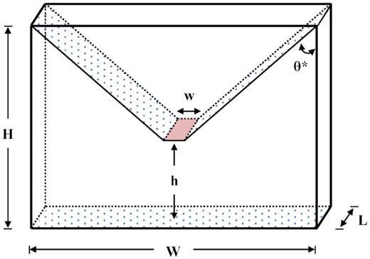
Schematic of the experimental container used for the piling experiments and simulations. Patterned surfaces are covered with fixed 1 mm glass beads. The container height H is 177 mm, the container width W is 126 mm, the container length L is 18 mm, the slot width w is 13 mm, the distance from the slot opening to the floor h is 56 mm, and the ramp inclination |$\theta ^*$| is 50 deg.
5.2 Simulation set-up
The experiment container is re-created in chrono using plates and spheres. Particles are fixed to the top surfaces of the inclined ramps and floor, mimicking the frictional wall conditions in the experiment. The simulation is executed in two phases: a filling phase and a discharge phase. In the first phase, a funnel is constructed above the container using small, fixed particles. The funnel is filled by arranging particles in a loosely packed cloud and providing the particles with random initial velocities to promote mixing. The particles fall through the funnel into the container. The filling phase ends when the total kinetic energy of the system falls below |$1 \times 10^{-9}$| Joules. This energy level was selected to reduce computation time while ensuring that the simulation ends in a stable state. In the next phase, the centre divider slides back at a rate of 0.1 m s−1, allowing the particles to flow on to the container floor. The simulation ends when the total kinetic energy of the system once again falls below |$1 \times 10^{-9}$| Joules.
The parameters used for the piling simulations are listed in Table 2. Some of the material properties, like density and Poisson’s ratio, map directly to reference sheets for glass beads. The references do not match the exact beads used in the experiment, but are used because the properties should be comparable.
| Property | Symbol | Value | Reference |
|---|---|---|---|
| Time-step (|$\mu \mathrm{ s}$|) | t | 1.0 | (Huang, Nydal & Yao 2014) |
| Particle diameter (mm) | d | 1.0 |$\pm$| 0.2 | – |
| Particle density (kg m|$^{-3}$|) | |$\rho$| | 2500 | (Bolz 2019) |
| Young’s modulus (MPa) | E | 70 | (Chen et al. 2017; Bolz 2019) |
| Poisson’s ratio | |$\nu$| | 0.24 | (Bolz 2019) |
| Particle–particle coefficient of restitution | |$e_{\mathrm{ p}}$| | 0.97 | (Foerster et al. 1994) |
| Particle–wall coefficient of restitution | |$e_{\mathrm{ w}}$| | 0.82 | (Alizadeh, Bertrand & Chaouki 2014) |
| Particle–particle static friction coefficient | |$\mu _{\mathrm{ s,p}}$| | 0.16 | (Amstock 1997; Alizadeh et al. 2014) |
| Particle–wall static friction coefficient | |$\mu _{\mathrm{ s,w}}$| | 0.45 | (Alizadeh et al. 2014) |
| Particle–particle dynamic friction coefficient | |$\mu _{\mathrm{ k,p}}$| | 0.16 | (Alizadeh et al. 2014) |
| Particle–wall dynamic friction coefficient | |$\mu _{\mathrm{ k,w}}$| | 0.45 | (Alizadeh et al. 2014) |
| Rolling friction coefficient | |$\mu _{\mathrm{ r}}$| | 0–0.2 | – |
| Spinning friction coefficient | |$\mu _{\mathrm{ t}}$| | 0 | – |
The true value of Young’s modulus, E, is estimated to be |$\sim$|70 GPa for glass beads (Bolz 2019). However, large estimates for E result in large stiffness coefficients, short collision durations, and the need for unrealistically small time-steps (see Appendix A and equations 27–29). An investigation into the effects of Young’s modulus on particle mixing in a tumbler found that E can be decreased by at least three orders of magnitude before variations in tumbler flow begin to develop (Chen et al. 2017). For expediency and consistency between simulations, E was adjusted to 70 MPa for the piling tests. The remaining parameters in Table 2 were selected based on experimental observations from previous works (Foerster et al. 1994; Amstock 1997; Alizadeh et al. 2014; Chen et al. 2015).
5.3 Data processing
The experimental angle of repose is estimated using the image processing toolbox in Matlab. First, test images are contrasted and converted into binary format. Then, background noise and pixels belonging to the container are removed. The tail-ends and centre of the heap are also identified and removed so that their curvatures do not influence the angle measurement. Finally, the left and right repose angles are determined by fitting lines through the upper edges of the remaining pile.
The simulated angles of repose are found by flattening the final positions of the particles into a 2D plane and fitting a line through the uppermost bodies in the pile. As with the experimental data, the tail-end and centre portions of the heap are excluded from the line fit.
5.4 Results and observations
Using the method described in Section 5.3, the experimental angle of repose was measured as 25.2 |$\pm$| 0.8 deg across six trials. The error represents the standard deviation of the mean from the 12 angle measurements (two measurements, left and right, per trial). Fig. 6 shows side-by-side snapshots from the real and numerical tests. At a high level, the simulations succeed in reproducing the flow patterns observed in the experiments. Specific details related to angle of repose and flow behaviour will be discussed in the Sections 5.5 and 5.6. The simulations contain 58 040 particles and were executed on an Intel® Xeon® Gold 6140 processor using 36 OpenMP threads. The discharge phase of the simulations lasted 1.5 real seconds and took approximately 2000 cpu hours or 2.5 d on a single processor to complete.
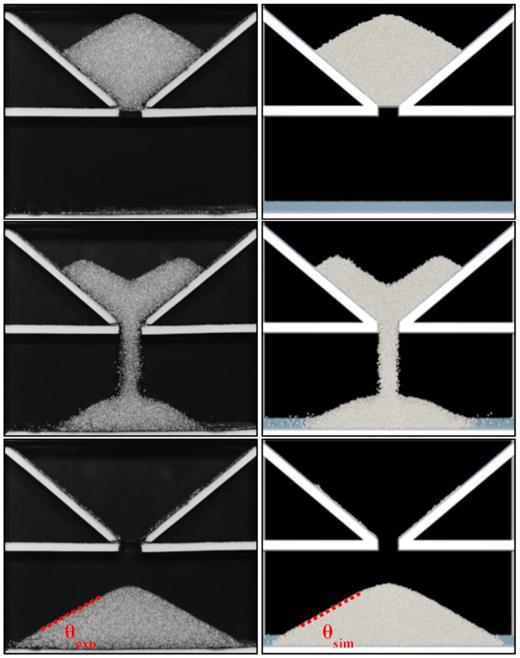
Snapshots from the beginning, middle, and end of the piling test, with experiment images on the left and simulation images on the right. The experimental angle of repose |$\theta _{\mathrm{ exp}}$| is 25.2 |$\pm$| 0.8 deg. When |$\mu _\mathrm{ r}$| = 0.09, the simulated angle of repose |$\theta _{\mathrm{ sim}}$| is 25.3 |$\pm$| 0.1 deg.
5.5 Angle of repose
Glass beads are frequently used for granular testing because their material properties are either well understood or are relatively easy to extract. Certain parameters, however, like the coefficients of rolling and spinning friction, are exceptions. Their values are related to specific resistance models, and they are therefore easiest to obtain by calibrating simulations against experimental data. In this study, we vary the coefficient of rolling friction between 0 and 0.2 to find the friction value that most accurately replicates the angle of repose observed in the piling experiments. In Fig. 7, we see that the angle of repose increases with rolling friction, and that the simulated pile matches the experimental pile most when |$\mu _\mathrm{ r} = 0.09$|. The trend where |$\theta$| increases and then levels off is consistent with findings from previous works (Zhou et al. 1999, 2002).
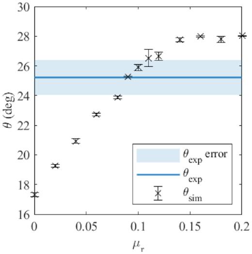
Angle of repose |$\theta$| for piling simulations with rolling friction coefficient |$\mu _\mathrm{ r}$| ranging from 0 to 0.2. Error bars represent the standard deviation of the mean between the left and right angle measurements. The simulations correspond best with experimental results when |$\mu _\mathrm{ r}$| = 0.09.
5.6 Flow behaviour
Unfortunately, it is difficult to calculate the theoretical discharge rate for the piling tests because of the irregularly shaped surface created by the filling process (see Fig. 6). None the less, simulation data can be used to find the total mass discharged over the duration of the simulation. In Fig. 8, we see the rate increases sharply at the beginning of the simulation, remains constant from t = 0.2 to 0.6 s, and then levels off at the end of the simulation. By comparing test cases where |$\mu _\mathrm{ r} = 0$| and |$0.09$|, we note that discharge rate decreases slightly as friction increases.
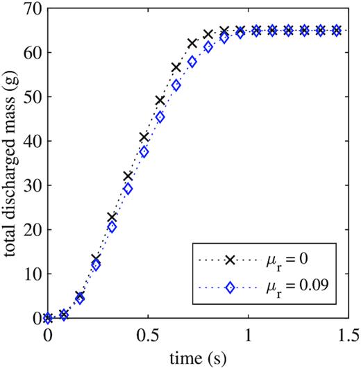
Total discharged mass during piling simulations with two different coefficients of rolling friction |$\mu _\mathrm{ r}$|.
Fig. 9 helps explain the why the mass discharge rate changes as it does. At t = 0.1 s, the slot is only partially open, and the majority of the particle beds are static. Mass discharge increases sharply as the slot opens. From t = 0.15 to 0.35 s, the particles above the slot sink at a uniform speed until they near the orifice. Particle velocities around the orifice increase as the bodies converge and fall through the slot. Mass discharge is nearly constant during this period. At t = 0.45, very few particles remain in the static zone, and the mass discharge rate decreases as the remaining particles exit the system. Qualitatively, the flow matches expected results (Anand et al. 2008; Schwartz et al. 2012; Yan et al. 2015).
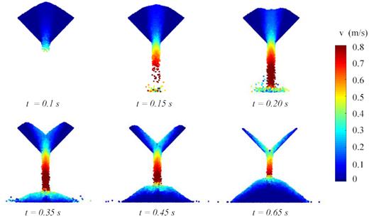
Snapshots of particle flow during the piling simulation when |$\mu _\mathrm{ r} = 0.09$|. Particles are coloured by velocity magnitude.
6 TUMBLER FLOW TEST
Tumbler flow is a significant area of research in granular mechanics. Authors have used rotating drums to study mixing and segregation (Dury & Ristow 1997; Gray & Thornton 2005; Xu et al. 2010; Chen et al. 2017), to understand the impact of particle size, shape, and friction on flow behaviour (Alizadeh et al. 2014; Chou, Hu & Hsiau 2016; Santos et al. 2016), to calibrate material properties in DEM simulations (Hu, Liu & Wu 2018), and to explore the effects of boundary conditions on particle motion (Dury et al. 1998; Félix, Falk & D’Ortona 2002). Thanks to the abundance of information on the topic, tumbler flow has become a key benchmarking study for DEM code validation. In this section, we numerically replicate tumbler experiments performed by Brucks et al. (2007). We vary the drum rotation speed, gravity level, particle size, particle friction, and contact model to validate the code against expected behaviours. Then, we use chrono to investigate the effects of cohesion on flow velocity and regime transitions.
6.1 Analytical theory
Particles can transition through six flow states in a rotating drum: slipping, slumping, rolling, cascading, cataracting, and centrifuging (Henein, Brimacombe & Watkinson 1983a). The regimes are characterized by different flow patterns, while transitions between the regimes are influenced by parameters like material properties, the tumbler rotation speed, the ratio of drum length to particle diameter (L/d), the ratio of drum diameter to particle diameter (D/d), the drum fill ratio (Henein, Brimacombe & Watkinson 1983b; Mellmann 2001). Behaviour in the rolling and cascading regimes can be compared in more detail by looking at the flowing layer velocity, flowing layer thickness, and dynamic angle of repose. In this study, the dynamic angle of repose is defined as the angle from horizontal where the surface-layer particles flow at a constant slope (see Fig. 11).
Brucks et al. (2007) explore the relationship between gravity level, drum rotation speed, and angle of repose by conducting a series of tumbler experiments inside of a centrifuge. The authors measure the dynamic angle of repose and the flowing layer thickness for tests with two different drum sizes, drum rotation speeds reaching up to 25 rad s−1, and gravity levels ranging from |$1g_\mathrm{ o}$| to |$25g_\mathrm{ o}$|, where |$g_\mathrm{ o}$| is Earth’s gravity or 9.81 m s−2. For more information on the experimental set-up, we refer the reader to Brucks et al. (2007). When plotting the angle of repose as a function of Froude number, they found that their data collapse on to a single curve. In the following sections, we perform simulations to see if a similar trend is obtained when |$g \lt 1g_\mathrm{ o}$| as when |$g \ge 1g_\mathrm{ o}$|.
Both Gravity level and grain size play key roles in determining whether a granular system is gravity dominated or cohesion dominated. In the absence of moisture content, particles must be sub-millimetre sized or smaller in order for cohesion to influence a granular system on the Earth (Walton, De Moor & Gill 2007). Conversely, cohesion can in principle become important on small-body surfaces for centimetre sized or larger grains, due to reduced-gravity levels (Scheeres et al. 2010). For example, using equations (15) and (32) where gravity level g = 0.0057 m s−2 and cleanliness factor S = 0.88, the Bond number for regolith on Phobos, a moon of Mars, nears unity for grains that are approximately 3 cm in diameter. Using different parameters and a notably smaller cleanliness factor, Hartzell, Farrell & Marshall (2018) find that cohesive forces come into play for 1 mm or smaller grains on Phobos. In Section 6.4.4, we investigate the effects of cohesion on reduced-gravity systems by simulated tumbler flow when |$g \le g_\mathrm{ o}$| and |$Bo \ge 1$|.
6.2 Simulation set-up
The simulations discussed in this section loosely mimic experiments performed by Brucks et al. (2007), where the drum dimensions match the smaller of the two test set-ups described in the paper. In each simulation, a 60 mm diameter drum is half-filled with particles and rotated at a constant angular velocity. A frictional wall condition is modelled by creating the drum’s inner cylinder out of particles. The inner particle ring rotates as an assembly with the front and back plates. The drum is 5 mm in length and contains either 0.53 |$\pm$| 0.05 or 1.0 |$\pm$| 0.05 mm particles following a normal size distribution. Tests with the smaller particles provide a direct comparison against experimental data, but are computationally expensive due to the large number of particles in the system. Since the Brucks et al. (2007) experiments use glass beads, all other simulation parameters are identical to those used in Section 5 (see. Table 2).
At the start of the simulation, particles are loosely packed inside of the drum and are provided with random initial velocities in order to generate collisions and promote mixing. Once settled, any particles sitting above the drum’s centre line are removed to ensure a half-filled drum state (see Fig. 10).
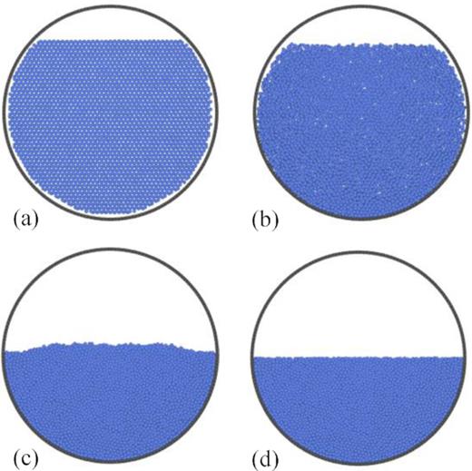
Snapshots of the tumbler during simulation set-up. (a) Particles are loosely arranged in the drum, (b) provided with initial velocities so that they mix, and then (c) left to settle under gravity. (d) Particles on the surface of the bed are removed so that the drum is half-filled.
Then, the container is rotated at a constant velocity for 5 s, or until the system’s total kinetic energy converges to a certain value when the particles are in a flowing state. The axis of rotation passes through the centre of the container and is parallel to the axis of the cylinder. All simulations were executed using 20–36 OpenMP threads on an Intel® Xeon® Gold 6140 processor.
6.3 Data processing
Particle positions and velocities are reported in 0.01 s intervals and are used to determine the dynamic angle of repose, the velocity field, and the flowing layer thickness for different test cases. The dynamic angle of repose |$\theta$| is calculated from the best-fitting line that passes through the top layer of the particle bed. A mean angle is calculated across 1 simulation second, and the error is reported as the standard deviation of the mean. As Froude number increases, the flowing surface evolves from a flat shape into an S-shaped curve (see Section 6.4.1). The steep angles found at the tail-ends of the S-curve are excluded from the |$\theta$| measurement by sampling the position data within a D/2 perimeter about the centre of the drum, as shown by the thick red lines in Fig. 11.
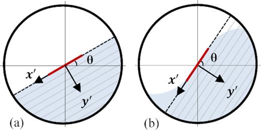
Diagram showing the coordinate system used for the analysis of simulations with (a) |$Fr = 1\times 10^{-4}$| and |$1\times 10^{-3}$| and (b) |$Fr = 1\times 10^{-2}$| to 0.1. The angle of repose |$\theta$| is measured at the centre of the drum (shown by the thick red line), and the streamwise velocities are averaged within the regions running parallel to the |$x^\prime$| direction. The spin vector is directed out of page.
Once the mean repose angle has been measured, particles are binned into regions to construct a streamwise velocity profile. The regions, illustrated in Fig. 11 with dotted lines, run parallel to the surface and are approximately two particle diameters thick. Particle velocities in the |$x^\prime$| direction are averaged within each region and used to construct a profile for flow velocity |$v_x^\prime$| as a function of distance |$y^\prime$| from the free surface. Finally, flowing layer thickness |$y^\prime _{\mathrm{ fl}}$| is defined as the distance along |$y^\prime$| where the flow reverses direction, indicated by the intersection of the velocity profile with |$x^\prime =0$|. Alizadeh et al. (2014) describe methods for determining |$y^\prime _{\mathrm{ fl}}$| in more detail.
6.4 Results and observations
A summary of the tumbler test cases and results is provided in Table 3. Angle of repose and flowing layer thickness are reported when |$Fr\, \le$| 0.1. When |$Fr \gt 0.1$|, |$\theta$| and |$y^\prime _{\mathrm{ fl}}$| cannot be measured because the flow falls into the cataracting and centrifuging regimes. Sections 6.4.1–6.4.3 discuss the simulation results in more detail.
Summary of test cases and results for the tumbler simulations discussed in Section 6, where d is the particle diameter, L is the drum length, |$\omega$| is the drum rotation speed, |$C_3$| is the cohesion multiplier for the Perko et al. (2001) cohesion model, g is the gravity level, |$g_\mathrm{ o}$| is the Earth gravity, |$Fr$| is the Froude number, |$Bo$| is the cohesive Bond number, |$\mu _\mathrm{ r}$| is the coefficient of rolling friction, |$\theta$| is the dynamic angle of repose, and |$y^\prime _{\mathrm{ fl}}$| is the flowing layer thickness. All other simulation parameters are listed in Table 2.
| d (mm) | |$L/d$| | particles | model | |$\omega$| (rpm) | |$C_3$| (g s−2) | g | |$Fr$| | |$Bo$| | |$\mu _\mathrm{ r}$| | |$\theta$| (deg) | |$y^\prime _{\mathrm{ fl}}$| |
|---|---|---|---|---|---|---|---|---|---|---|---|
| 0.53 | 9.4 | 64 453 | Hertz | 1.7 | 0 | |$g_\mathrm{ o}$| | 0.0001 | 0 | 0.09 | 31.8 |$\pm$| 0.8 | 3.5 |
| 0.53 | 9.4 | 64 453 | Hertz | 5.4 | 0 | |$g_\mathrm{ o}$| | 0.001 | 0 | 0.09 | 32.7 |$\pm$| 0.9 | 4.5 |
| 0.53 | 9.4 | 64 453 | Hertz | 17 | 0 | |$g_\mathrm{ o}$| | 0.01 | 0 | 0.09 | 41.1 |$\pm$| 0.3 | 6.0 |
| 0.53 | 9.4 | 64 453 | Hertz | 39 | 0 | |$g_\mathrm{ o}$| | 0.05 | 0 | 0.09 | 53.5 |$\pm$| 0.3 | 7.8 |
| 0.53 | 9.4 | 64 453 | Hertz | 55 | 0 | |$g_\mathrm{ o}$| | 0.1 | 0 | 0.09 | 59.2 |$\pm$| 0.4 | 9.0 |
| 0.53 | 9.4 | 64 453 | Hertz | 122 | 0 | |$g_\mathrm{ o}$| | 0.5 | 0 | 0.09 | – | – |
| 0.53 | 9.4 | 64 453 | Hertz | 173 | 0 | |$g_\mathrm{ o}$| | 1.0 | 0 | 0.09 | – | – |
| 0.53 | 9.4 | 64 453 | Hertz | 212 | 0 | |$g_\mathrm{ o}$| | 1.5 | 0 | 0.09 | – | – |
| 1.0 | 5 | 9 228 | Hertz | 1.7 | 0 | |$g_\mathrm{ o}$| | 0.0001 | 0 | 0.09 | 32.1 |$\pm$| 0.6 | 4.2 |
| 1.0 | 5 | 9 228 | Hertz | 1.7 | 51.37 | |$g_\mathrm{ o}$| | 0.0001 | 1 | 0.09 | 37.2 |$\pm$| 1.7 | 4.6 |
| 1.0 | 5 | 9 228 | Hertz | 5.4 | 0 | |$g_\mathrm{ o}$| | 0.001 | 0 | 0 | 26.1 |$\pm$| 0.6 | 5.4 |
| 1.0 | 5 | 9 228 | Hertz | 5.4 | 0 | |$g_\mathrm{ o}$| | 0.001 | 0 | 0.09 | 35.0 |$\pm$| 0.6 | 4.9 |
| 1.0 | 5 | 9 228 | Hooke | 5.4 | 0 | |$g_\mathrm{ o}$| | 0.001 | 0 | 0.09 | 31.8 |$\pm$| 0.7 | 4.6 |
| 1.0 | 5 | 9 228 | Flores | 5.4 | 0 | |$g_\mathrm{ o}$| | 0.001 | 0 | 0.09 | 35.1 |$\pm$| 0.7 | 5.0 |
| 1.0 | 5 | 9 228 | Hertz | 5.4 | 51.37 | |$g_\mathrm{ o}$| | 0.001 | 1 | 0.09 | 37.1 |$\pm$| 0.9 | 4.8 |
| 1.0 | 5 | 9 228 | Hertz | 17 | 0 | |$g_\mathrm{ o}$| | 0.01 | 0 | 0.09 | 41.4 |$\pm$| 1.1 | 6.5 |
| 1.0 | 5 | 9 228 | Hertz | 17 | 51.37 | |$g_\mathrm{ o}$| | 0.01 | 1 | 0.09 | 42.9 |$\pm$| 0.7 | 6.2 |
| 1.0 | 5 | 9 228 | Hertz | 39 | 0 | |$g_\mathrm{ o}$| | 0.05 | 0 | 0.09 | 51.5 |$\pm$| 0.9 | 8.2 |
| 1.0 | 5 | 9 228 | Hertz | 39 | 51.37 | |$g_\mathrm{ o}$| | 0.05 | 1 | 0.09 | 53.3 |$\pm$| 0.6 | 8.2 |
| 1.0 | 5 | 9 228 | Hertz | 55 | 0 | |$g_\mathrm{ o}$| | 0.1 | 0 | 0.09 | 57.2 |$\pm$| 0.7 | 9.3 |
| 1.0 | 5 | 9 228 | Hertz | 55 | 51.37 | |$g_\mathrm{ o}$| | 0.1 | 1 | 0.09 | 58.3 |$\pm$| 0.7 | 9.3 |
| 1.0 | 5 | 9 228 | Hertz | 122 | 0 | |$g_\mathrm{ o}$| | 0.5 | 0 | 0.09 | – | – |
| 1.0 | 5 | 9 228 | Hertz | 173 | 0 | |$g_\mathrm{ o}$| | 1.0 | 0 | 0.09 | – | – |
| 1.0 | 5 | 9 228 | Hertz | 212 | 0 | |$g_\mathrm{ o}$| | 1.5 | 0 | 0.09 | – | – |
| 1.0 | 5 | 9 228 | Hertz | 3.8 | 0 | |$5g_\mathrm{ o}$| | 0.0001 | 0 | 0.09 | 32.2 |$\pm$| 0.7 | 4.1 |
| 1.0 | 5 | 9 228 | Hertz | 3.8 | 256.8 | |$5g_\mathrm{ o}$| | 0.0001 | 1 | 0.09 | 37.3 |$\pm$| 2.1 | 4.6 |
| 1.0 | 5 | 9 228 | Hertz | 3.8 | 0 | |$0.5g_\mathrm{ o}$| | 0.001 | 0 | 0.09 | 34.9 |$\pm$| 0.5 | 5.0 |
| 1.0 | 5 | 9 228 | Hertz | 3.8 | 12.84 | |$0.5g_\mathrm{ o}$| | 0.001 | 0.5 | 0.09 | 36.0 |$\pm$| 0.6 | 5.0 |
| 1.0 | 5 | 9 228 | Hertz | 3.8 | 25.68 | |$0.5g_\mathrm{ o}$| | 0.001 | 1 | 0.09 | 37.0 |$\pm$| 0.7 | 4.7 |
| 1.0 | 5 | 9 228 | Hertz | 3.8 | 51.37 | |$0.5g_\mathrm{ o}$| | 0.001 | 2 | 0.09 | 39.1 |$\pm$| 1.0 | 4.6 |
| 1.0 | 5 | 9 228 | Hertz | 3.8 | 77.05 | |$0.5g_\mathrm{ o}$| | 0.001 | 3 | 0.09 | 44.5 |$\pm$| 3.1 | 5.1 |
| 1.0 | 5 | 9 228 | Hertz | 3.8 | 102.7 | |$0.5g_\mathrm{ o}$| | 0.001 | 4 | 0.09 | 35.0 |$\pm$| 2.5 | 4.8 |
| 1.0 | 5 | 9 228 | Hertz | 3.8 | 205.5 | |$0.5g_\mathrm{ o}$| | 0.001 | 8 | 0.09 | – | – |
| 1.0 | 5 | 9 228 | Hertz | 3.8 | 0 | |$0.05g_\mathrm{ o}$| | 0.01 | 0 | 0.09 | 42.1 |$\pm$| 1.6 | 6.5 |
| 1.0 | 5 | 9 228 | Hertz | 3.8 | 2.568 | |$0.05g_\mathrm{ o}$| | 0.01 | 1 | 0.09 | 43.1 |$\pm$| 0.4 | 6.3 |
| 1.0 | 5 | 9 228 | Hertz | 3.8 | 0 | |$0.01g_\mathrm{ o}$| | 0.05 | 0 | 0.09 | 52.3 |$\pm$| 0.6 | 8.6 |
| 1.0 | 5 | 9 228 | Hertz | 3.8 | 0.503 | |$0.01g_\mathrm{ o}$| | 0.05 | 1 | 0.09 | 53.4 |$\pm$| 0.6 | 8.5 |
| 1.0 | 5 | 9 228 | Hertz | 3.8 | 0 | |$0.005g_\mathrm{ o}$| | 0.1 | 0 | 0.09 | 57.5 |$\pm$| 1.8 | 10.4 |
| 1.0 | 5 | 9 228 | Hertz | 3.8 | 0.252 | |$0.005g_\mathrm{ o}$| | 0.1 | 1 | 0.09 | 58.6 |$\pm$| 1.5 | 10.6 |
| 1.0 | 5 | 9 228 | Hertz | 3.8 | 0 | |$0.001g_\mathrm{ o}$| | 0.5 | 0 | 0.09 | – | – |
| 1.0 | 5 | 9 228 | Hertz | 3.8 | 0 | |$0.0005g_\mathrm{ o}$| | 1.0 | 0 | 0.09 | – | – |
| 1.0 | 5 | 9 228 | Hertz | 3.8 | 0 | |$0.0003g_\mathrm{ o}$| | 1.5 | 0 | 0.09 | – | – |
6.4.1 Flow behaviour
Fig. 12 depicts the evolution of flow behaviour with increasing Froude number. Each image represents a snapshot taken at the end of a simulation, where particles are coloured by normalized velocity magnitude. At |$Fr = 1\times 10^{-4}$| and |$1\times 10^{-3}$|, the drum motion produces a thin flowing layer at a relatively constant repose angle. The particles in the flowing layer are moving faster than the drum itself, indicating that the flow is in the rolling regime. The flow transitions from the rolling to cascading regime at |$Fr$| = 0.01. In the cascading regime, the surface particles assume the expected S-curved shape. At |$Fr$| = 0.5, the flow enters the cataracting regime, where particles rise to a steep angle along the drum wall before detaching and falling back to the bottom of the drum. Finally, by |$Fr$| = 1.5, the flow has transitioned into the centrifuging regime. At high Froude numbers, particles are thrown against the inner wall of the drum and rotate at the same velocity as the container. The observed flow patterns match the predicted motion and transition behaviours described in Mellmann (2001) and Henein et al. (1983b).
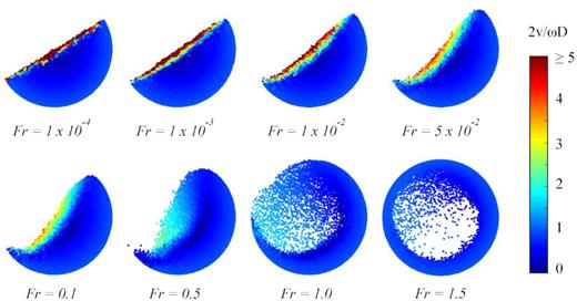
Stead-state flow patterns at different Froude numbers for tumbler simulations where d = 1 mm, |$\mu _\mathrm{ r} = 0.09$|, and |$g = 1g_\mathrm{ o}$|. Particles are coloured by velocity magnitude, normalized by drum diameter D and drum rotation speed |$\omega$|. The flow is in the rolling regime when |$Fr = 1\times 10^{-4}$| and |$1\times 10^{-3}$|, in the cascading regime when |$Fr$| ranges from |$1\times 10^{-2}$| to 0.1, and in the cataracting regime when |$Fr$| = 0.5. The flow is transitioning into the centrifuging regime when |$Fr$| = 1.0 and 1.5.
6.4.2 Angle of repose
Simulations with 0.53 mm particles and a 60 mm drum were carried out to provide a full-scale comparison with the Brucks et al. (2007) experiments. The simulations cover a range of Froude numbers by holding gravity-level constant at 1|$g_\mathrm{ o}$| while varying drum velocity from 1.7 to 212 rpm. The trend of increasing |$\theta$| with |$Fr$| shown in Fig. 13 matches experimental data, but the magnitudes of the repose angles are of the order of 5–7 deg higher than that observed in the physical tests. One explanation for the discrepancy could be a mismatch in material properties between the real and simulated beads. Previous studies have found that sliding, rolling, and wall friction have the biggest influences on tumbler flow behaviour, while Young’s modulus, Poisson’s ratio, and coefficient of restitution are less important, given that the values fall within reasonable ranges (Qi et al. 2015; Yan et al. 2015; Chou et al. 2016). Another explanation for the discrepancy could be that the particles fixed along the inside of the drum walls result in a more influential boundary condition than created by the walls of the experimental drum, which were lined with 60-grit sandpaper.
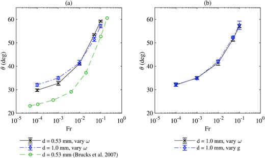
Dynamic angle of repose |$\theta$| for tumbler simulations with different Froude numbers. Plot (a) compares simulation results against data from Brucks et al. (2007). Plot (b) shows simulation results when the Froude number is obtained by varying either drum rotation speed or gravity level (see equation 31). In one test set, |$\omega$| varies from 1.7 to 55 rpm. In the other, g varies from |$0.005g_\mathrm{ o}$| to |$5g_\mathrm{ o}$|.
Each full-scale simulation takes approximately 4000 cpu hours or 5 d on a single processor to complete. To reduce computation time, all remaining simulations were conducted using 1 mm diameter particles. Increasing particle size while keeping drum diameter fixed reduces the number of particles in the system from about 64 500 to 9200. A comparison between the repose angles for the two different particle sizes can be found in Fig. 13. Experiments have shown that the repose angle either decreases or remains constant when drum to particle diameter (D/d) increases, at least for low rotational velocities (Dury et al. 1998; Liu, Specht & Mellmann 2005; Brucks et al. 2007). A similar phenomenon occurs when the ratio of drum length to particle diameter (L/d) increases (Dury et al. 1998; Yang et al. 2008). Consistent with these findings, the simulations with the 1.0 mm particles reach higher repose angles than those with the 0.53 mm particle when |$Fr \lt 0.01$|. When |$Fr \gt 0.01$|, the trend changes, and higher repose angles are observed for the smaller particles. Dury et al. (1998) reported the same outcome when investigating the effects of boundary conditions on repose angle. At lower Froude numbers, particles are more densely packed and lose the bulk of their energy through frequently occurring collisions. As Froude number increases, however, the particle bed dilates and collision frequency decreases (Yang et al. 2008). Extrapolating from this line of thought, it is possible that friction and boundary conditions are more influential at lower Froude numbers, where the particles are more constrained and inter-particle interactions dominate the flow.
The above tests cover a range of drum rotation speeds, but only one gravity level. Since |$\theta$| is dependent on both |$\omega$| and g, varying gravity instead of rotation speed should produce the same results. To verify, more simulations were executed with drum rotation speed fixed at 3.8 rpm and gravity level ranging from |$3.2 \times 10^{-4}g_\mathrm{ o}$| to |$5g_\mathrm{ o}$|. As expected from the Brucks et al. (2007) experiments, the repose angles collapse on to a single curve (see Fig. 13).
6.4.3 Velocity profile in the rolling regime
Rolling friction is varied in order to understand the influence of |$\mu _\mathrm{ r}$| on the simulation results. Tests are conducted within the rolling regime, at Fr = |$1\times 10^{-3}$|, so that streamwise velocities can be compared in addition to repose angles. The tests show that |$\theta$| increases more than 5 deg when |$\mu _\mathrm{ r}$| changes from 0 to 0.09 (see Table 3). The higher angles produce more energetic particles, increasing the average velocity on the bed’s surface (see Fig. 14). In Table 3, an increase in |$\theta$| typically coincides with an increase in flowing layer thickness. However, |$y^\prime _{\mathrm{ fl}}$| is actually lower when |$\mu _\mathrm{ r}$| = 0.09 than when |$\mu _\mathrm{ r}$| = 0. This is because energy dissipates more quickly through the bed when the total contact torque takes into account a rolling resistance moment. Rolling friction increases the rate of velocity change through the flowing layer and reduces the flowing layer thickness. These results match findings from Chou et al. (2016), who conduct a detailed investigation into the effects of friction on tumbler flow.
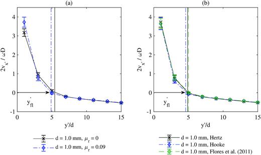
Average streamwise velocity |$v_x^\prime$| as a function of distance from the free surface for tumbler simulations where d = 1.0 mm. The vertical lines on the plot depict flowing layer thickness |$y^\prime _{\mathrm{ fl}}$|. The streamwise velocity is normalized by drum rotation speed |$\omega$| and drum diameter D, and the distance from the free surface is normalized by particle diameter d. Plot (a) shows the velocity profiles for tests with the Hertz force model and different rolling friction coefficients and plot (b) compares results for different force models when |$\mu _\mathrm{ r}$| = 0.09. The higher rolling friction leads to increased velocity at the free surface while the different force models show little to no variation in the velocity profile.
The Hooke, Hertz, and Flores et al. (2011) force models are also compared at |$Fr = 1\times 10^{-3}$| and |$\mu _\mathrm{ r}$| = 0.09. The streamwise velocity profiles for the three models are similar, suggesting that the non-physical behaviour associated with the Hookean and Hertzian models has little impact on the bulk response of the system (see Fig. 14). Additional testing is required to determine if this observation holds across different applications and flow states.
6.4.4 Flow behaviour with cohesion
The tests presented in Sections 6.4.1–6.4.3 neglect inter-particle cohesion. Here, we use the Perko et al. (2001) cohesion model to explore how cohesion influences flow behaviour and dynamic angle of repose for simulations under both Earth-gravity and reduced-gravity levels. First, we vary cohesion while leaving the gravity-level constant at |$0.5g_\mathrm{ o}$| and the drum rotation speed constant at 3.8 rpm. The Froude number for the given configuration is 0.001, and the cohesion multiplier |$C_3$| is selected such that the granular Bond number ranges from 0.5 to 8 (see Table 3). Fig. 15 illustrates the flow patterns and the normalized flow velocities for tests where |$Bo$| = 0, 2, 4, and 8. The top row of the figure corresponds to the time t where the system reaches a maximum stable angle before experiencing its first avalanche (|$t = t^*$|) and the bottom row shows the state of the system 0.1 s later (|$t = t^* + 0.1$| s). The time difference between the top and bottom images corresponds to a small angular distance and was selected simply to illustrate the material’s transition from a semisolid state to a flowing state.
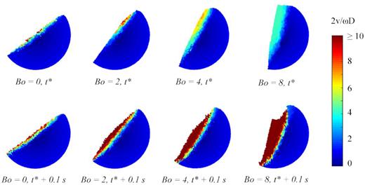
Flow patterns for simulation with different granular Bond numbers when d = 1 mm, |$\mu _\mathrm{ r}$| = 0.09, |$g = 0.5g_\mathrm{ o}$|, |$\omega$| = 3.8 rpm, and |$Fr$| = 0.001. Particles are coloured by velocity magnitude, normalized by drum diameter D and drum rotation speed |$\omega$|. |$t^*$| is the time where the system reaches a maximum stable angle before experiencing its first avalanche.
The flow behaviour when |$Bo$| = 0 is consistent with the rolling regime, as evident from the thin, fast-moving layer on the surface of the bed. As the Bond number, increases however, the flow undergoes several observable changes. First, the particles begin to avalanche in clusters rather than individually. The larger the Bond number, the larger the collapsing cluster. Once the flow is initiated (i.e. at |$t = t^* + 0.1$| s), the surface profile evolves from being flat or slightly concave at |$Bo$| = 0 to convex at |$Bo$| = 2 and 4 and to irregularly shaped at |$Bo$| = 8. Additionally, the thickness of the high-velocity flowing region on the surface of the bed increases as |$Bo$| increases.
Shortly after flow initiates, the behaviour reaches a steady state. In Fig. 16(a), we plot the dynamic angle of repose as a function of the Bond number. As expected, both the dynamic angle of repose and the maximum stable angle of repose increase as the Bond number increases. The error bars on the angle measurements are large when |$Bo$| = 2, 3, and 4, indicating that the system experiences periodic avalanching at higher cohesion values. Observations regarding the collapse/avalanching behaviour, the surface profiles, the angle of repose, and the flowing-layer velocity are qualitatively consistent with findings from previous experiments and simulations performed at |$1g_\mathrm{ o}$| (Nase et al. 2001; Walton et al. 2007; Brewster, Grest & Levine 2009; Chou & Hsiau 2011; Liu, Yang & Yu 2013; Jarray et al. 2017; Jarray et al. 2019).
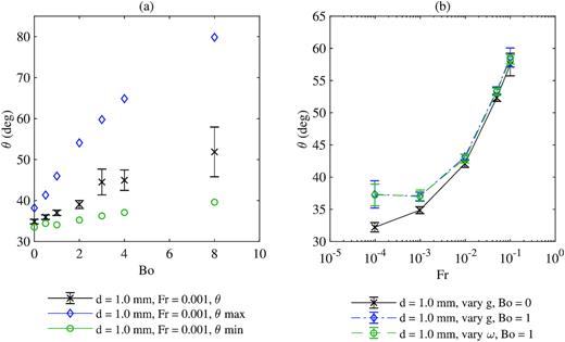
Dynamic angle of repose |$\theta$| for tumbler simulations with different Froude and Bond numbers. The error bars represent the standard deviation of the mean |$\theta$| measurement over 1 real second of stead-state flow, while |$\theta$| max and |$\theta$| min are the before and after angle measurements for the flow’s first avalanche. Plot (a) compares simulations with different Bond numbers when |$g = 0.5g_\mathrm{ o}$| and |$\omega$| = 3.8 rpm. Plot (b) shows simulation results when Froude number is obtained by varying either drum rotation speed or gravity level. In one test set, |$\omega$| varies from 1.7 to 55 rpm. In the others, g varies from |$0.005g_\mathrm{ o}$| to |$5g_\mathrm{ o}$|.
In the next set of tests, we check if the relationship between the dynamic angle of repose and the Froude number holds when inter-particle cohesion is non-zero. Like in Section 6.4.2, the Froude number is controlled by varying either the drum rotation speed or the gravity level. For test cases where |$Bo$| = 1 and |$g = g_\mathrm{ o}$|, |$\omega$| ranges from 1.7 to 55 rpm and the cohesion multiplier |$C_3$| remains constant at 51.37 g s−2. For test cases where |$Bo$| = 1 and |$\omega = 3.8$| rpm, the gravity level ranges from |$0.005g_\mathrm{ o}$| to |$5g_\mathrm{ o}$| and |$C_3$| varies from 0.252 to 256.8 g s−2 (see Table 3).
Fig. 16(b) shows the dynamic angle of repose plotted as a function of the Froude number for the second set of simulations. The data collapse on to a single curve for all cases where |$Bo$| = 1, just as it did for the cohesionless system (see Fig. 13). In Fig. 16(b), we also see that the dynamic angle of repose is slightly higher when |$Bo$| = 1 than when |$Bo$| = 0, though the difference is more pronounced at lower Froude numbers. Based on the results from the first cohesion test and a study by Walton et al. (2007), we would expect the angle gap between the cohesionless and cohesion-dominated system to grow as |$Bo$| increases until some critical Bond number is reached. Above that critical number, the material would stop flowing and would fall apart in clumps or would simply rotate as a solid body.
Nase et al. (2001) conducted a piling, a hopper flow, and a tumbler study with wet granular material and controllable levels of capillary cohesion. The authors found that the static angle of repose and the discharge rate for the piling and the hopper tests change drastically as soon as the Bond number exceeds a |$Bo$| = 1 threshold. However, their experimental data show that the dynamic angle of repose for the tumbler tests does not jump or change dramatically when |$Bo \ge 1$|. Consequently, Nase et al. (2001) cannot distinguish a clear transition between the flowing and cohesive states in the tumbler using the Bond number alone as a characterization tool. Like Nase et al. (2001), our tests show a gradual increase in |$\theta$| as |$Bo$| increases. This suggests that in addition to gravitational and cohesive forces, shearing and collision forces play non-negligible roles in certain granular phenomena. Much more work is required to understand impacts of cohesion on different types of flows.
7 CONCLUSIONS
The SSDEM code in chrono::parallel 4.0.0 was modified to include the Flores et al. (2011) force model and the Perko et al. (2001) cohesion model, and to account for rolling and spinning friction. These enhancements are relevant for both terrestrial and planetary science applications and are publicly available as chrono version 5.0.0. The code changes were validated using a combination of two-body and multibody benchmarking tests. The two-body tests reveal that the normal, tangential, and cohesive force calculations are correctly implemented in the code, and that the sliding, rolling, and spinning models yield the expected behaviours.
In Section 5, we compared experimental and numerical results for a ‘sand piling’ test using 1 mm glass beads. We varied the coefficient of rolling friction in the simulations, and found that as expected, the pile’s angle of repose increases as |$\mu _\mathrm{ r}$| increases. The angle of repose given by the simulations best matches the experimental data when |$\mu _\mathrm{ r} = 0.09$|.
Finally, in Section 6, we present the results for the rotating drum simulations. We varied, among other parameters, gravity level and cohesion, noting that solid bodies in our Solar system, from asteroids to planets, cover a wide range of gravity conditions. Overall, the simulation results match findings from other experimental and numerical works. We observe that the drum flow spans the rolling, cascading, cataracting, and centrifuging regimes when the Froude number |$Fr$| increases from |$1\times 10^{-4}$| to 1.5 (see Fig. 12). The regime transitions occur at the expected value of |$Fr$|, regardless of how |$Fr$| is controlled (i.e. by changing rotational velocity or by changing gravity level). The angle of repose and the flowing layer thickness were measured when |$Fr\, \le$| 0.1. When all parameters aside from |$Fr$| are held constant, |$\theta$| and |$y^\prime _{\mathrm{ fl}}$| increase with |$Fr$|. Otherwise, subtle differences are observed when particle size, rolling friction coefficient, and force model are varied. Flow patterns and regime transitions change when cohesion is introduced into the system, and the dynamic angle of repose increases as the granular Bond number increases. The simulation results with cohesion are also in agreement with previous experimental works.
The SSDEM model in chrono::parallel accurately replicates known granular flow behaviours, even for varied gravity and cohesion levels. As part of future work, this platform will be used to study regolith dynamics and lander–surface interactions. This upcoming work will aid with the interpretation of surface-regolith images sent by current and past missions (e.g. Hayabusa2 and OSIRIS-REx) and will help prepare for future ones, like JAXA’s MMX mission to Phobos and Deimos and ESA’s Hera mission to the binary asteroid Didymos.
ACKNOWLEDGEMENTS
We would like to thank Dan Negrut and Radu Serban at the University of Wisconsin-Madison and the chrono developers for their support and collaboration. We would also like to acknowledge José Andrade and the Computational Geomechanics group at the California Institute of Technology for allowing us to use their laboratory equipment and facilities, and Lennart Klar for assisting with early code development. This project uses High-Performance Computing resources from the CALMIP supercomputing center in Toulouse, France, under grant allocation 2019-P19030, and is jointly funded by the Centre National d’Etudes Spatiales (CNES) and the Institut Supérieur de l’Aéronautique et de l’Espace (ISAE) under a PhD research grant. Naomi Murdoch, Stephen Schwartz, and Patrick Michel acknowledge funding support from the Centre National d’Etudes Spatiales (CNES). Patrick Michel and Stephen Schwartz acknowledge funding from Academies of Excellence: Complex systems and Space, Environment, Risk, and Resilience, part of the Initiative of Excellence University (IDEX) Joint, Excellent and Dynamic Initiative (JEDI) of the Université Côte d’Azur. Stephen Schwartz acknowledges grant number 80NSSC18K0226 as part of the OSIRIS-REx (Origins, Spectral Interpreta- tion, Resource Identification, and Security-Regolith Explorer) Participating Scientist Programme.
DATA AVAILABILITY
The data underlying this article will be shared on a reasonable request to the corresponding author.
