


ABSTRACT
We present observations and models of the kinematics and the distribution of the neutral hydrogen (H i) in the isolated dwarf irregular galaxy, Wolf-Lundmark-Melotte (WLM). We observed WLM with the Green Bank Telescope (GBT) and as part of the MeerKAT Early Science Programme, where 16 dishes were available. The H i disc of WLM extends out to a major axis diameter of 30 arcmin (8.5 kpc), and a minor axis diameter of 20 arcmin (5.6 kpc) as measured by the GBT. We use the MeerKAT data to model WLM using the tirific software suite, allowing us to fit different tilted-ring models and select the one that best matches the observation. Our final best-fitting model is a flat disc with a vertical thickness, a constant inclination and dispersion, and a radially varying surface brightness with harmonic distortions. To simulate bar-like motions, we include second-order harmonic distortions in velocity in the tangential and vertical directions. We present a model with only circular motions included and a model with non-circular motions. The latter describes the data better. Overall, the models reproduce the global distribution and the kinematics of the gas, except for some faint emission at the 2σ level. We model the mass distribution of WLM with pseudo-isothermal (ISO) and Navarro–Frenk–White (NFW) dark matter halo models. The NFW and the ISO models fit the derived rotation curves within the formal errors, but with the ISO model giving better reduced chi-square values. The mass distribution in WLM is dominated by dark matter at all radii.
1 INTRODUCTION
The circular rotation speed of stars or gas in galaxies around their centre of mass is mainly set by the balance between the galaxy’s centrifugal force and its gravitational force (Roberts & Rots 1973). Therefore, the shape of the rotation curve of a galaxy can be used to model its mass distribution. When the circular velocities of the ionized gas in the spiral galaxy M31 were measured (at optical wavelength) as a function of the radial distance from the galaxy’s centre in the 1970s by Rubin & Ford (1970), it was realized that the measured rotation curve did not follow what was expected from the distribution of the visible matter in the galaxy. In fact, instead of following a Keplerian decline, the rotation curve rose sharply in the inner disc and remained flat at larger distance. A flat rotation curve was later observed in a number of spiral galaxies at even larger distance from the centre than previously achieved using the hyperfine 21 cm line emission of neutral hydrogen (H i) gas (Roberts & Rots 1973; Peterson et al. 1978; Bosma 1981; van Albada et al. 1985; Sofue & Rubin 2001; Carignan et al. 2006; de Blok et al. 2008). This result strengthened the idea that the observed matter in galaxies cannot account for the total gravitational force that holds matter in galaxies. Therefore, there must be invisible matter in the halo of spiral galaxies that contributes to the total orbital speed of the gas and the stars. This unseen mass is known as dark matter, whose very first observational evidence came from the study of the Coma cluster in the 1930s by Fritz Zwicky. Understanding the role and the properties of dark matter is at the heart of modern cosmology. The decomposition of the galaxy’s rotation curve in terms of the contribution from visible matter (stars and gas) and dark matter has become a powerful tool to model the mass distribution in both spiral and dwarf galaxies (Carignan & Freeman 1985; Carignan et al. 2006; de Blok et al. 2008; Oh et al. 2011; Oh 2012; Randriamampandry & Carignan 2014; Namumba et al. 2019). Dwarf galaxies are dominated by dark matter even inside their optical discs (Carignan & Beaulieu 1989; Oh et al. 2011). Therefore, their inferred central dark matter density distributions are less affected by the uncertainties due to the assumed contribution of baryonic matter to the total dynamical mass and the mass-to-light ratio of the stellar discs (Iorio et al. 2017). However, their kinematics are usually affected by non-circular motions and therefore analysing their mass distributions requires careful kinematical modelling (Oh et al. 2008).
Several models are proposed in the literature to explain the distribution of dark matter in galaxies. The most popular ones are the Navarro–Frenk–White model (NFW; Navarro, Frenk & White 1996) and the pseudo-isothermal model (ISO; Begeman 1987). The NFW model was derived from N-body simulations of collisionless cold dark matter haloes and is characterized by a steep power-law mass-density distribution (known as the cusp model). The ISO model is motivated by observations and is characterized by a shallow inner mass-density profile (the core model). Despite being dark matter dominated, the rotation curves of dwarf and low-surface brightness galaxies have been found to be inconsistent with the cosmologically motivated NFW cuspy profile (but see Oman et al. 2019; Kurapati et al. 2020). Instead, they are best fitted by the ISO model. This is known as the core-cusp problem; an extensive review on this can be found in de Blok (2010). In this paper, we use both the NFW and ISO models to model the dark matter distribution of the dwarf irregular (dIrr) galaxy, Wolf-Lundmark-Melotte (WLM, DDO 221, UGCA 444), using H i as mass and kinematics tracers. We map the H i gas in WLM using the MeerKAT radio telescope. This paper presents the first MeerKAT data in its 32k mode. To estimate the completeness of the emission recovered by MeerKAT, we compare the flux recovered by MeerKAT with the flux recovered by observations using the 100 m Robert C. Byrd Green Bank Telescope (GBT). We model the distribution and kinematics of the H i in WLM using sophisticated 3D modelling techniques implemented in the software package tirific1 (Józsa et al. 2007).
The shapes of the rotation curves of galaxies can be influenced by several factors: inherent in the data itself (beam smearing, pointing offsets, and non-circular motions; see Oh et al. 2008) and also in the method applied (1D versus 2D versus 3D method). One of the widely used approaches to derive a rotation curve consists of extracting a velocity that best represents the circular motion of the gas along each line of sight. By doing so, one gets a map of the representative velocities along all lines of sight (i.e. a velocity field). The extracted velocity field can then be fitted with a tilted-ring model to obtain the rotation curve. This approach is known as the 2D velocity field method and is implemented in many software packages, such as in the gipsy task ROTCUR (Begeman 1987; Spekkens & Sellwood 2007), DiskFiT (Sellwood & Sánchez 2010), and most recently the software 2DBAT (Oh et al. 2018). As mentioned in Oh et al. (2008), the 2D velocity-field approach requires the projection of a 3D data cube to an infinitely thin disc. While this makes the computation faster, it has some limitations. These include beam smearing, the presence of non-circular motions, the inability to model the vertical thickness of the disc, and to simulate the case where the sightline crosses the disc multiple times, the most extreme case of this being edge-on galaxies (Oh et al. 2008). Beam smearing tends to lower the true rotation velocity, whereas the assumption of a thin disc may overestimate the rotation curve at the outer radius (Bosma 1978; Burlak, Gubina & Tyurina 1997; Kregel & van der Kruit 2004; Swaters et al. 2009). In addition, the presence of non-circular motions, which manifests itself as kinks in the velocity fields, makes the derivation of rotation curves uncertain, especially for dwarf galaxies where the kinematics can be severely affected by non-circular motions (Bosma 1978; Oh et al. 2008; Trachternach et al. 2008). For this analysis, we opt for the 3D approach due to its great flexibility to make a complex model, it is less affected by beam smearing effects, and its ability to work even in the presence of strong non-circular motions. The 3D method consists of directly fitting a tilted-ring model to the data cube (Józsa et al. 2007; Di Teodoro & Fraternali 2015; Kamphuis et al. 2015) in order to extract kinematic information such as the rotation velocity, the velocity dispersion, and the surface brightness profile. We use the derived rotation curve from our tilted-ring model to model the luminous and dark matter distributions in the galaxy. This analysis will contribute to our understanding of the dark matter distribution in dwarf galaxies.
We organize our paper as follows. In Section 2, we describe the properties of WLM. In Section 3, we present the observation set-up. In Section 4, we present the data reduction procedures. In Section 5, we contrast our observations with archival optical data. In Section 6, we describe our kinematical modelling methods and present the kinematic parameters. In Section 7, we present the mass modelling of the galaxy. In Section 8, we discuss the results, and in Section 9, we give a summary.
2 PROPERTIES OF WLM
WLM is a dIrr galaxy in the Local Group. It was first discovered by Wolf (1909), and later identified as a nebula by Lundmark (unpublished) and Melotte (1926) when analysing Franklin-Adams Charts Plates, thus the name Wolf-Lundmark-Melotte or, in short, WLM. A tip of the red giant branch analysis placed it at a distance of 0.97 Mpc (Karachentsev, Makarov & Kaisina 2013), close enough to have allowed detailed studies of its stellar population and star formation history. Using the Hubble Space Telescope data, Dolphin (2000) reported that WLM formed half of its stellar population earlier than 9 Gyr ago. This was followed by a gradual decrease in star formation until 1–2.5 Gyr ago after which a rise in activity was observed. WLM star formation continues until the present epoch but is confined in what appears to be a bar in the centre of the galaxy (Dolphin 2000). Despite having a metallicity 50 per cent lower than the reported carbon monoxide (CO) detection threshold, Rubio et al. (2015) found 10 CO clouds with an average radius of 2 pc and an average virial mass of 103 M⊙ in WLM using the Atacama Large Millimetre Array. Rubio et al. (2015) also noted that WLM formed stars efficiently despite its low CO content. The basic properties of WLM are presented in Table 1.
| WLM | ||||
|---|---|---|---|---|
| Parameters | Symbols | Values | Units | Ref. |
| Morphological type | – | dIrr | – | 1 |
| Optical centre | RA | 00|$\rm {^{h}}01\rm {^{m}}$| 58.1|$\rm {^{s}}$| | – | 2 |
| (J2000) | Dec | −15° 27′ 40″ | – | 2 |
| Systemic velocity | vsys | |$-122\, \pm \, 4$| | |$\mathrm{km}\, \mathrm{s}^{-1}$| | 3 |
| Distance | d | 0.97 | Mpc | 2 |
| B-band magnitude | MB | −13.56 | mag | 4 |
| Stellar mass | M⋆ | 4.3 × 10⁷ | M⊙ | 4 |
| Star formation rate | SFR(FUV) | 0.008 | |$\mathrm{ M}_\odot \, \mathrm{yr}^{-1}$| | 5 |
| Optical diameter | D25 | 1.98 | kpc | 5 |
| Optical position angle | PAopt | 4 | ° | 4 |
| H i diameter | |$D_\mathrm{ H}\, {\small I}$| | |$15.\!\!^\prime 8\, \pm \, 1.\!\!^\prime 2$| | – | 3 |
| H i diameter | |$D_\mathrm{ H}\, {\small I}$| | |$4.3\, \pm \, 0.4$| | kpc | 3 |
| |$D_\mathrm{ H}\, {\small I}$|/D25 | 2.17 | – | 3 | |
| Total H i mass | |$M_\mathrm{ H}\, {\small I}$| | |$5.5\, \pm \, 0.6\cdot 10^7$| | M⊙ | 3 |
| Rotation velocity | |$v_\mathrm{rot}(r_\mathrm{ H}\, {\small I})$| | |$29\, \pm \, 5$| | |$\mathrm{km}\, \mathrm{s}^{-1}$| | 3 |
| Dyn. mass | |$M_\mathrm{dyn}(r_\mathrm{ H}\, {\small I})$| | |$4.0\, \pm \, 1.4\cdot 10^8$| | M⊙ | 3 |
| H i line width | W50 | |$54\, \pm \, 11$| | |$\mathrm{km}\, \mathrm{s}^{-1}$| | 3 |
| |$W^\mathrm{c}_{50}$| | |$55\, \pm \, 10$| | |$\mathrm{km}\, \mathrm{s}^{-1}$| | 3 | |
| W20 | |$85\, \pm \, 14$| | |$\mathrm{km}\, \mathrm{s}^{-1}$| | 3 | |
| |$W^\mathrm{c}_{20}$| | |$84\, \pm \, 13$| | |$\mathrm{km}\, \mathrm{s}^{-1}$| | 3 | |
WLM has previously been observed in H i. Using the GBT, Hunter et al. (2011) mapped its H i disc and measured an H i diameter of 28 arcmin at |$\rm {10^{19}~cm^{-2}}$|. This is about 2.4 times the optically defined Holmberg diameter and is in good agreement with the previous VLA H i observation by Kepley et al. (2007). Kepley et al. (2007) found that the H i distribution of WLM is not uniform, but has a hook-like structure of high column density in the centre, encompassing roughly 20 per cent of the total H i mass. The origin of this feature is not clear but is most likely due to active star formation in the centre that blows out or ionizes the gas. According to Kepley et al. (2007), the H i velocity field of WLM is asymmetric, with the northern part appearing to be warped.
WLM appears to have evolved in isolation, free from significant external encounters. This is because WLM lies far away from its nearest neighbour, the Cetus dwarf spheroidal galaxy. They are separated from each other by a distance of 250 kpc (Leaman et al. 2011). Note that the size of WLM is approximately 8 kpc as traced by H i emission (Kepley et al. 2007; Hunter et al. 2011). A search for possible H i companions around WLM by Barnes & de Blok (2004) was unsuccessful. Leaman et al. (2012) classified WLM as among the five least tidally disturbed and one of the most isolated galaxies within 1 Mpc of the Milky Way. Thus, WLM is an interesting target for at least three main reasons. First, it is a gas-rich dwarf galaxy with a very extended H i disc, allowing us to trace its gravitational potential out to very large radius. Secondly, being a gas-rich dIrr galaxy, it falls within a mass range where cold gas accretion is still expected to occur (Schmidt et al. 2014). Lastly, its isolated nature enables the description of the radial and vertical velocity structures of the disc without being hampered by the presence of debris or irregular kinematics.
3 OBSERVATIONS
3.1 MeerKAT
The MeerKAT H i observations of WLM were conducted with the L-band (900–1670 MHz) receivers of the MeerKAT-16 telescope (Jonas & MeerKAT Team 2018), composed of 16, 13.5 m dishes, with a maximum baseline of 8 km as part of the MeerKAT Early Science observations. The target was observed for about 5.65 h, including overheads. A total bandwidth of 856 MHz centred at 1283.98 MHz was recorded and was divided into 32k channels with a channel width of 26.12 kHz each and two linear polarizations. The target field was observed for a total time of 3.15 h in multiple scans of 13.5 min at 16 s integration time. Moreover, 2.5 h were spent on three calibrator sources: J1938-6341 and J0408-6544 for bandpass calibration, and J0003-1727 for gain (amplitude and phase) calibration. We summarize the observing set-up in Table 2.
MeerKAT H i observations of WLM galaxy.
| Property | Value |
|---|---|
| Number of antennas | 16 |
| Total observation time (h) | 5.65 |
| Frequency range (MHz) | 900–1670 |
| Central frequency (MHz) | 1285 |
| Bandpass calibrator 1 | J1938-6341 [19:39:25–63:42:45] |
| Bandpass calibrator 2 | J0408-6544 [04:08:20–65:44:09] |
| Gain calibrator | J0003-1727 [00:03:22–17:27:14] |
| Number of channels | 4098 |
| Channel width (kHz) | 26.123 |
| Central frequency (MHz) | 1420.9893 |
To achieve the required sensitivity, the 16 MeerKAT antennas were arranged such that 12 antennas formed part of a compact configuration, and the remaining 4 antennas were at a distance of more than 1000 m from the core, resulting in an extended beam of up to 60 arcsec. The few chosen extended baselines allowed a better estimate of the bandpass and phase solutions. The quasi-random distribution of antennas allowed us to attain imaging of suitable quality, despite the proximity of WLM to the equator. In addition, the MeerKAT primary beam full width at half-maximum (FWHM) at 1.4 GHz is significantly larger than the H i diameter of WLM, allowing us to map its extended emission without mosaicking.
3.2 GBT
4 DATA PROCESSING
4.1 MeerKAT
We reduced the MeerKAT data using the Containerised Automated Radio Astronomy Calibration pipeline2 (CARACal; formerly known as MeerKATHI; Józsa et al. 2020), being developed in an international collaboration, with main contributions coming from Rhodes University, the South African Radio Astronomy Observatory (SARAO), and the Italian National Institute for Astrophysics. CARACal has initially been developed to reduce the MeerKAT data, but its scope is intentionally to be able to reduce data from any radio interferometers. CARACal performs different data reduction steps (flagging, calibration, and imaging) using standard radio astronomy data reduction tools such as casa (Brogan et al. 2007), AOFlagger (Offringa et al. 2010), WSClean (Offringa et al. 2014), CubiCal (Kenyon et al. 2018), etc. in containerized environments provided by a python-based scripting framework called Stimela.3 The advantages of using CARACal include reproducibility of results, highly customizable, and the ability to use a wide variety of data analysis tools in a seamless manner.
4.1.1 Flagging and calibration
We perform the data reduction within CARACal using a chunk of 50 MHz around the WLM central H i emission frequency with a width of 26.12 KHz, resulting in a data set of 1915 channels. Prior to cross-calibration of the data, the known RFI-prone channels are flagged using a baseline-independent flagging mask obtained from SARAO. To remove emission from the Milky Way, the channels corresponding to the Milky Way’s emission frequencies are flagged using the casa task flagdata. This is the default setting of CARACal and is appropriate for a galaxy far away from the Galactic plane like WLM. After flagging, cross-calibration is performed. This includes delay calibration, as well as bandpass and gain calibrations. The casa task SETJY is used to determine the flux density of the flux calibrator J1938-6341. The casa task BANDPASS is used to correct for instrumental delays. We estimate a maximum delay correction of 1.5 ns, which is standard for MeerKAT. To estimate the time-dependent antenna-based gain and to solve for the phase, the casa tasks gaincal and bandpass are used, respectively.
After cross-calibration, the data get processed through a set of four self-calibration steps. In each step, the data go through a WSClean imaging and calibration using CubiCal. The clean components produced by WSClean are used to make a sky model for the calibration. To avoid the selection of artefacts in the mask, we start with shallow cleaning and then iteratively go deeper by lowering the auto-mask and the auto-threshold parameters in CARACal until all sources are detected and the residuals are noise-like. To compute image statistics such as the dynamic range and moments of distribution of residuals in the successive self-cal steps, we enabled the image-based quality assessment tool aimfast. These quantities are used as stopping criteria for the self-calibration processes. Our self-calibration strategy improves the dynamic range of the images and allows a better model of the continuum sources.
4.1.2 Continuum subtraction and imaging
To examine the astrometry and the flux density fidelity of the continuum images of the WLM field, we compare the positions and flux densities of the sources in the field with the equivalent quantities in the NRAO Very Large Array (VLA)4 Sky Survey (NVSS; Condon et al. 1998) for the same sources.
We use the PyBDSF source finder (Mohan & Rafferty 2015) on our continuum images (with the default settings, which we find satisfactory) to construct a source catalogue for the WLM field. From this catalogue, only the sources with the code ‘S’ are chosen, from which we found 64 sources. These sources are single-Gaussian sources that are the only sources in their respective ‘islands’ (Mohan & Rafferty 2015). We compare the position and the integrated flux densities of these sources with those in the catalogue of the NVSS. The results are presented in Figs 1 and 2. There is an excellent agreement between the flux densities recovered by our MeerKAT-16 observation and those recovered by the VLA NVSS survey. The mean positional offsets in RA and DEC are 0.05 and −0.07 arcsec, with standard deviations of 0.9 and 0.7 arcsec, respectively. We find no systematic trends in RA and DEC and conclude that the WLM field source positions well match those of the NVSS catalogue.

Comparison of the flux densities of matched sources in the MeerKAT-16 WLM field and the NVSS catalogue.

Positional offsets in RA and DEC between sources in our MeerKAT-16 WLM field and the corresponding matched sources in the NVSS catalogue.
4.2 GBT
The standard data reduction was done with AIPS6 and the gbtidl7 routine (Marganian et al. 2006). The gbtidl data reduction steps for frequency-switched spectral line data are described in detail in Pingel et al. (2018), and here we follow the same procedure as they adopted. We smoothed the data from their native resolution of 3.1 kHz to a channel width of 24.4 kHz (5.2 km s−1) using a boxcar function. The rms noise in the final cube was 32 mJy beam−1. This corresponds to a column density of 4 × 1018 cm−2 (3σ detections over 2 channels of 5.2 km s−1 width, and a beam size of ∼9 arcmin).
5 H i AND OPTICAL DATA
5.1 Total flux and global H i profile
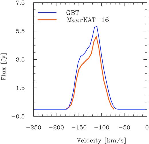
Global H i velocity profiles of WLM from the GBT data (blue) and the MeerKAT data (red).
5.2 Moment maps and optical data
5.2.1 GBT
For the GBT, the moment zero map is of particular interest to estimate the extent of the H i disc. We use SoFiA to obtain the moment zero map, and from which we derive a column density map. Pixels below the 3σ rms noise level are blanked. In Fig. 4, we overplot the column density map of WLM on to an archival optical image from the Digitised Sky Survey (DSS).8 As shown by the white arrows in the figure, the H i extends out to a major axis diameter of ∼30 arcmin (∼8.5 kpc), and a minor axis diameter of ∼20 arcmin (5.6 kpc). These values have been derived at a column density level of 6.2 × 1018 cm−2. Our measured H i diameter is slightly larger than the extent derived by Hunter et al. (2011), who also used the GBT. However, it is in agreement with the value obtained by Kepley et al. (2007).

GBT column density map of WLM, overplotted on an archival DSS (red, IIIa-F) optical image. Contour levels are (0.62, 1.25, 2.50, 3.74, 4.99, 6.24, 7.49, 8.73, 9.98, 11.23, 12.48 13.73, 14.98, 16.22, 17.47, 18.72) × 1019 cm−2. The white cross represents the kinematical centre of the model derived from this study. The beam of the GBT observation is shown as the black circle.
5.2.2 MeerKAT
We use the miriad task MOMENT to derive the moment maps of the MeerKAT data. In Fig. 5, we overplot the surface density map of the low-resolution data cubes on to the DSS optical images of WLM. We show the optical image at its native resolution and after a convolution with a 2D Gaussian with an FWHM of 6 arcsec. The outermost contour shows the H i surface brightness level at 1 M⊙ pc−2; thus, it delimits the H i diameter quoted in Table 1. As observed in many gas-rich dwarf galaxies, the H i extends much farther than the optical disc. We derive an H i-to-optical diameter (DH i/D25) ratio of 2.17. The overall H i distribution is asymmetric, with the southern side slightly twisted towards the east.

Top left: column density map; contour levels are (0.9, 2.8, 8.4, 14.0, 25.2, 50.5, 59.0) |$\times ~10^{19}~\rm {cm}^{-2}$|. Top right: first moment map; contour levels are spaced by 10 km s−1 and start from −35 to 35 km s−1 relative to the systemic velocity vsys = −121.62 km s−1. Bottom left: second moment map. The beam (60 arcsec) is represented by the grey circle at the bottom left of the first three panels. Bottom right: H i spectra from the high-resolution data cube of WLM (35 arcsec × 12 arcsec). The spectra are separated from each other by a distance of 45 arcsec in the x- and y-directions. The background grey-scale image shows |$\rm {H\,{\alpha }}$| emission from the SPITZER/LVL archive.
We present the column density map, the first moment map (velocity field), and the second moment map in Fig. 6. The H i column density distribution appears to be smooth in the outer disc. However, in the central part, there are a few high-column density peaks whose location closely matches that of the H α emission observed as part of the Spitzer Local Volume Legacy project9 (Dale et al. 2009). The hook-like morphology observed by Kepley et al. (2007) is not recovered by our observations but the location of the high-column density peaks roughly matches that of the hook. The velocity field shows twisted iso-velocity contours in both the Northern and Southern sides. While the twisted, curved iso-velocity contours in the Northern side were seen previously in high-resolution observations (Jackson et al. 2004; Kepley et al. 2007), the ones in the Southern side did not show up due to the limited sensitivity of these observations. They indicate a warp-like morphology but their origin is not clear given that WLM is an isolated galaxy. The inner iso-velocity contours are mostly parallel to the minor axis, indicating a solid-body rotation. Signatures of differential rotation, indicated by curved iso-velocity contours, are found slightly further away from the centre. As reported by Kepley et al. (2007), here also we find that the inner approaching halve of the galaxy shows steeper velocity gradient than the inner receding side. For the second moment map, there are regions with enhanced second moment values in the Southern side, corresponding to the location of the warp suggested by the moment-1 velocity field. The inner north-east side also has regions of higher second moment values. This corresponds to the region where we find a few double-peaked profiles. The central and far Northern sides have lower second moment values than the rest of the pixels. Regions with enhanced second moment values have been attributed to turbulence effects caused by, e.g. star formation feedback or magneto rotational instability (Tamburro et al. 2009). Investigating the origin of this pattern of high second moment values requires pixel-by-pixel analysis of the shapes of the H i spectrum, which is beyond the scope of this analysis.

H i surface density map of WLM overlaid on top of the DSS (red, IIIa-F) images of WLM. Top: the DSS image is shown at its native resolution. Bottom: the DSS image has been convolved with a 2D Gaussian of |$\mathrm{ FWHM}\, =\, 6$| arcsec in each direction. Blue contours denote the H i surface density at |$1,9\,$| |$\mathrm{ M}_\odot \, \mathrm{pc}^{-2}$| levels. The white crosses represent the kinematical centre of the model. The beam of the MeerKAT-16 observation is shown as black circles in each panel.
WLM has experienced an initial burst of star formation, and continues to form stars until the present epoch (Albers et al. 2019). Therefore, we may expect to see expanding shells of gas produced by past supernova explosions in WLM. We look for possible signatures of such shells in the star-forming disc of WLM. For this, we use the high-resolution data cube, which has a spatial resolution of 163 × 56 pc. Supernova-driven shells, which appear as H i holes with size above our linear resolution limit, are common in spirals and dwarf galaxies (Boomsma et al. 2008; Bagetakos et al. 2011; Warren et al. 2011). Thus, if expanding shells with size above our linear resolution are present in WLM, we would expect to see their imprints on the H i kinematics. We use the H α image from the IRAC/LVL10 archive to trace the location of star formation. Signatures of expanding shells include the presence of double-peaked H i spectra, and enhanced velocities at the radius of the shell. At the bottom right of Fig. 6, we show individual H i spectra in the central region of WLM where the H α emission occurs. Virtually, all profiles inside the region are single peaked, except in the North-Eastern side where we find a few double-peaked profiles. This location also corresponds to the region where we find high second moment values as mentioned previously. In addition to looking at the shapes of the individual profiles, we used the Karma-kshell11 tool to search for enhanced velocity signatures around the expected centre of the shells but our findings were inconclusive. Thus, at our resolution limit of 163 × 56 pc, we do not find any convincing evidence that the H i is currently expanding in single star formation regions in WLM.
6 3D MODELLING
To model the global kinematics and the morphology of WLM, we fit the data with an extended version of the tilted-ring model of Rogstad, Lockhart & Wright (1974) implemented in the tirific software suite. tirific allows the user to fit a tilted-ring model directly to the data cube instead of a velocity field, as is done in classic tilted-ring fitting method. tirific has the advantage of having a larger set of parameters compared to the velocity-field-based approach. This enables the user to explore different combinations of model parameters and makes a more complex modelling where necessary.
6.1 Modelling strategy
tirific models a galaxy as a rotating disc of radius R, with a thickness that follows a certain distribution in the vertical direction. The disc is divided into a set of TIRNR circular, concentric rings with widths RADSEP, each centred at (XPOS, YPOS), tilted at an inclination of INCL with respect to the sky plane and oriented at a position angle defined by the PA parameter. Each ring simulates rotating gas with a surface brightness distribution SBR, a circular velocity VROT, a systemic velocity VSYS, and a velocity dispersion SDIS. The user can specify the number of discs to be modelled using the NDISKS parameter. Parameters that correspond to a particular disc number are then denoted by the parameter names followed by an underscore and the disc number. Fixing one or more parameters with radius makes the model simpler and allows a faster computing time. Thus, as described in Józsa (2007), Saburova et al. (2013), Schmidt et al. (2014), and Henkel et al. (2018), we start with a simple model and compare the result with the observation. If the simplest possible model does not sufficiently describe the observations, then we allow one or more parameters to vary with radius and check if that improves the model. If no significant improvements are found, we set the corresponding parameters to remain fixed. We therefore model the galaxy with different sets of parameter combinations described as follows. We assume that all rings (nodes) have the same rotation centre and the same systemic velocity. We further assume that the H i is optically thin. We then explore the following parameter set-up:
with fixed or radially varying position angle,
with fixed or radially varying inclination angle,
with fixed or radially varying disc thickness,
with or without global vertical and radial motion,
excluding or including second-order harmonic distortions in tangential and radial motions. This has been used in the literature to simulate bar-like motions (e.g. Franx, van Gorkom & de Zeeuw 1994; Schoenmakers 1999; Spekkens & Sellwood 2007; Saburova et al. 2013).
with or without first-order distortions in surface brightness,
with or without first- and second-order distortions in surface brightness.
6.2 Results
After a visual inspection of the previously described parameter combinations, our final best-fitting model is described as an optically thin H i disc with the following parameters:
one rotation centre and one systemic velocity for all rings,
a constant position angle and inclination,
a constant velocity dispersion,
a fixed disc thickness,
- a radially varying surface brightness with first- and second-order harmonic distortions described bywhere r is the radius, θ is the azimuthal angle, and SM1A/SM2A and SM1P/SM2P are the amplitudes and the phases of the distortions, respectively.(10)$$\begin{eqnarray*} \Sigma (r,\theta) &=& SBR(r)+SM1A(r)\times \cos (\theta -SM1P(r))+\nonumber \\ && SM2A(r)\times \cos (2(\theta -SM2P(r))), \end{eqnarray*}$$
a radially varying rotation velocity,
a radially varying tangential and radial velocity with second-order harmonic distortions. To keep a minimal number of parameters, the angle between the phase of the radial and tangential velocities was kept at an angle of 45°.
The harmonic distortions in surface brightness are required to model the asymmetric morphology of the galaxy and to describe the bar-like motions as used in Spekkens & Sellwood (2007) and Saburova et al. (2013). However, we find it necessary to only include the kinematic distortions from a radius of 120 arcsec. While adding a warp did not improve our results significantly, a thick disc of 85 arcsec (∼400 pc) was required to refine the model. In addition, the inclusion of non-circular motions improved the model and resulted in a more well-behaved rotation curve with less wiggles compared to the rotation curve from the model with only circular motions. Therefore, our final best-fitting model is the one with non-circular motions and without a warp, which we use for the mass modelling. However, for the interested readers, we present below comparison between different models.
6.2.1 The final flat-disc model versus a warp model
In Fig. 7, we show residual channel maps. The top panel shows a warp model (i.e. with a radially varying inclination and position angle) minus the observed data cube, whereas the bottom panel shows the final (flat-disc) model minus the observed data cube. In general, the final flat-disc model performs better in the Northern side compared to the warp model. Inversely, the warp model works best in the Southern side. For example, the bottom panels of Fig. 7 show elongated excess model emission (positive contours) adjacent to negative contours at v = (−95.3, −89.8, −84.3) km s−1. This indicates a warp that is not well recovered by the flat-disc model in the Southern part (as also indicated by the velocity field shown in Fig. 6). Overall though, the final flat-disc model is able to recover the general distribution of the emission while still keeping a minimal number of model parameters.

Residual channel maps. Top: a warp model minus the observed data cube; Bottom: the final (flat-disc) model minus the observed data cube. Contour levels are (−2.2, −1.1, 1.1, 2.2) × 0.005 Jy beam−1. Light blue contours show negative pixels.
6.2.2 The final (flat-disc) model with non-circular motions versus the (flat-disc) model with only circular motions
To compare the final model including non-circular motions with the model allowing for only circular motions, we show residual channel maps of the two models in Fig. 8. In addition, we show a channel-by-channel comparison of the observed data cube with the two model data cubes in Fig. 9. Overall, both models seem to perform equally better in reproducing the overall distribution of the gas. The discrepancies between the two models are only mostly apparent at the 2σ rms noise level, where the final model is to be preferred. Note that including the 2σ level emission in the fitting does not affect the modelling results in a systematic way but rather shows the relative strength of the models to fit faint extended emission.

Residual channel maps. Top: the circular (flat-disc) model minus the observed data cube; bottom: the final (flat-disc) model minus the observed data cube. Contour levels are (−2.2, −1.1, 1.1, 2.2) × 0.005 Jy beam−1. Light blue contours show negative pixels.

Individual channel maps of the tirific models overlaid on the observed data shown as blue contours. Contours denote the |$-2,2,6,18,54\, -\, \sigma _\mathrm{rms}$| levels, where |$\sigma _\mathrm{rms}\, =\, 5\, \mathrm{mJy}\, \mathrm{beam}^{-1}$|. Dashed lines represent negative intensities. Top: the tirific model allowing for only circular motions. Bottom: our final best-fitting model with non-circular motions. Crosses represent the kinematical centre of the models. The circles shown in the lower left side of each panel represent the synthesized beam (HPBW).
In Fig. 10, we compare the moment maps from the tirific models with the moment maps from the observed data cubes The total-intensity map is well reproduced by both models. However, the model with circular motions clearly fails to recover the curved iso-velocity contours in the velocity field. This is a further evidence regarding the strength of the model with non-circular motions over the model with only circular motions.

Total-intensity maps (left-hand panels) and moment-1 velocity fields (right-hand panels) of the tirific models overlaid on to the observed data (blue contours). Top: the tirific model allowing for only circular motions. Bottom: the final tirific model with non-circular motions. For the total-intensity maps, contours denote the |$\frac{1}{3},1.0,3,9,27\,$| |$\, \mathrm{ M}_\odot \, \mathrm{pc}^{-2}$| levels. Arrows indicate the positions of slices along which the position–velocity diagrams in Figs 11 and 12 were taken. For the velocity fields, contours are spaced by 10 |$\mathrm{km}\, \mathrm{s}^{-1}$| and range from −35 to 35 |$\mathrm{km}\, \mathrm{s}^{-1}$| relative to the systemic velocity |$v_\mathrm{sys}\, =\, -122\, \mathrm{km}\, \mathrm{s}^{-1}$|. The crosses or the intersection between arrows A and C represents the kinematical centre of the model. The circles to the lower left of each panel show the synthesized beam (HPBW).
In Figs 11 and 12, we show position–velocity (PV) diagrams across cuts parallel to the major and minor axes of WLM shown in Fig. 10. Slices B and C show 2σ emission that is not reproduced by the models. Note that we have cleaned the data cube below the noise level. Thus, it is possible that they are real emission, but a follow-up study is required to confirm this. It is also interesting that for slice B, there are discrepancies between the models and the data even at the high-flux density contours. Gas at anomalous velocities is often attributed to star formation or intergalactic gas accretion.

Position–velocity diagrams taken along slices shown in Fig. 10. Contours denote the |$-2,2,6,18,54\, -\, \sigma _\mathrm{rms}$| levels, where |$\sigma _\mathrm{rms}\, =\, 5\, \mathrm{mJy}\, \mathrm{beam}^{-1}$|. Blue: the observed data cube. Strong orange: the tirific model allowing for only circular motion. Dashed lines represent negative intensities. The ellipse represents the velocity (2 channels) and the spatial resolution (|$\sqrt{\mathrm{ HPBW}_\mathrm{maj}*\mathrm{ HPBW}_\mathrm{min}}$|, where HPBWmaj and HPBWmin are the major and minor axes half-power beam widths, respectively).

Position–velocity diagrams taken along slices shown in Fig. 10. Contours denote the |$-2,2,6,18,54\, -\, \sigma _\mathrm{rms}$| levels, where |$\sigma _\mathrm{rms}\, =\, 5\, \mathrm{mJy}\, \mathrm{beam}^{-1}$|. Blue: the observed data cube. Pink: the tirific final model. Dashed lines represent negative intensities. The ellipse represents the velocity (2 channels) and the spatial resolution (|$\sqrt{\mathrm{ HPBW}_\mathrm{maj}*\mathrm{ HPBW}_\mathrm{min}}$|, where HPBWmaj and HPBWmin are the major and minor axes half-power beam widths, respectively).
6.2.3 Final model parameters
We present the final model parameters that do not vary with radius in Table 3. The radially varying parameters are presented in Fig. 13. We estimate the errors on the best-fitting parameters using a bootstrap method. In summary, we fit the data using a Golden-Section nested intervals fitting algorithm to derive the model parameters. Then, we generate many synthetic data sets by shifting the model parameters at a single node by a random value. After that, we fit each set using the same fitting routine as the real data. Finally, we calculate the standard deviations of the best-fitting parameters of the synthetic data and we use them as the standard errors for the model parameters quoted in Table 3 and shown as errorbars in Fig. 13. We derived a slowly rising solid-body rotation curve, which is typical for dwarf galaxies.

Final tirific model of the H i disc of WLM. SBR/SD: surface brightness or surface column density. The two lines denote r25 and |$r_\mathrm{ H}\, {\small I}$| (at the larger radius). SM1/2A: amplitude of a harmonic distortion in surface brightness/surface column density, first and second order. SM1/2P: phase of a harmonic distortion in surface brightness/surface column density, first and second order. VROT: rotation velocity. RO/RA2A: amplitude of a second-order harmonic distortion in velocity in tangential/radial direction. RA2P: phase (azimuth) of second-order harmonic distortion in velocity in radial direction. The phase for the distortion in tangential direction is shifted by 45° with respect to RA2P. The grey line is the result of a fit, in which the rotation curve was left to vary on the nodes shown as dots.
Tilted-ring parameters not varying with radius, final model.
| WLM: tirific radially invariant parameters | |||
|---|---|---|---|
| Parameter | Symbol | Value | Unit |
| Model centre | RA | |$0^\mathrm{h}\, 1^\mathrm{ m}\, 58.1^\mathrm{s} \, \pm \, 4^\mathrm{s}$| | – |
| (J2000) | Dec | |$-15^\mathrm{d}\, 27^\mathrm{m}\, 56^\mathrm{s}\, \pm \, 32^\mathrm{s}$| | – |
| Systemic velocity | vsys | |$-122\, \pm \, 4$| | |$\mathrm{km}\, \mathrm{s}^{-1}$| |
| Thickness | z0 | |$85^{\prime \prime }\, \pm \, 9^{\prime \prime }$| | – |
| Inclination | i | |$77^{\circ }\,\pm \, 6^{\circ }$| | – |
| Position angle | pa | |$174.3^{\circ }\, \pm \, 0.7^{\circ }$| | – |
| Dispersion | σv | |$7.9\, \pm \, 0.4$| | |$\mathrm{km}\, \mathrm{s}^{-1}$| |
7 MASS MODELS
In this section, we study the properties of the luminous and dark matter components in WLM. For the reason given previously, our mass modelling will be based on the rotation curve from the model that includes non-circular motions. The mass modelling result for the circular model is presented in the appendix. We model the observed rotation curve as the dynamical contributions of stars, gas, and dark matter halo. For this, we consider two widely used dark matter halo models, described in the next section. The quadratic sum of the rotation curves of these three components is then compared with observations to gauge the strength of the assumed models.
7.1 Asymmetric drift correction
WLM rotation curve after asymmetric drift correction.
| WLM: rotation curve | ||
|---|---|---|
| RAD | VROT | ERR |
| (kpc) | (km s−1) | (km s−1) |
| 0.00 | 0.00 | 0.00 |
| 0.29 | 11.55 | 4.99 |
| 0.58 | 17.09 | 4.96 |
| 0.87 | 19.16 | 4.54 |
| 1.16 | 26.64 | 5.81 |
| 1.45 | 28.71 | 5.79 |
| 1.75 | 28.24 | 5.87 |
| 2.04 | 31.66 | 4.11 |
| 2.33 | 31.97 | 4.95 |
| 2.62 | 26.73 | 5.13 |
| 2.91 | 31.65 | 4.34 |
| 3.20 | 25.56 | 5.36 |
Note. RAD (kpc): radius. VROT (km s−1): rotation curve after asymmetric drift correction. ERR (km s−1): error in VROT.
7.2 Contribution of the gas component
To model the contribution of the gas component to the total rotation curve, we first convert the surface brightness profiles obtained from tirific (see Section 6) to mass surface density profiles. Then, we scale the derived surface density profiles by a factor of 1.4 to take into account the presence of Helium and other metals. We show the gas surface densities in Fig. 14. Finally, we use the obtained gas density profiles to model the contribution of the gas component to the total rotation velocities using the gipsy task ROTMOD.

Left: H i surface density profile of WLM. Right: Stellar surface density profile of WLM.
7.3 Contribution of the stellar component
To estimate the stellar mass in galaxies, one needs to assume a stellar mass-to-light ratio, (Υ⋆), from stellar population synthesis models. As mentioned in Oh et al. (2015), this assumption drives the largest uncertainties associated with converting the luminosity profile to the mass density profile. For this study, we have adopted a mass-to-light ratio based on 3.6 μm light from Spitzer IRAC. The 3.6 μm images are less affected by dust compared to optical images and mostly trace stellar light from old stellar populations, which are dominant in late-type dwarf galaxies. Here we adopt a |$\Upsilon _{\star }^{3.6}$| value of 0.37 from Oh et al. (2015), which is found to be appropriate for late-type dwarf galaxies like WLM. This value was derived using the empirical relation between galaxy optical colours and Υ⋆ values based on stellar population synthesis models (Bell & de Jong 2001). The detailed derivation of the mass-to-light ratio is given in Oh et al. (2008).
7.4 Contribution of the dark matter component
where c = R200/Rs is a concentration parameter, and R200 is the radius where the density contrast with respect to the critical density of the Universe exceeds 200, roughly the virial radius; the characteristic velocity, V200, is the velocity at that radius (Navarro et al. 1996). The NFW mass density profile is cuspy in the inner parts and can be represented by ρ ∼ rα, where α = −1.
We use the outputs of ROTMOD as described previously as inputs for the gipsy task ROTMAS to decompose the rotation curves of WLM into luminous and dark matter components. We use the inverse square of the uncertainties in the input rotation curves as weights for the least-squares fit in ROTMAS. The quality of the ROTMAS fits is judged by the calculated χ2 values. We present the results of our mass modelling in Fig. 15 and Table 5 .

Mass distribution models of WLM with ISO (left-hand panel) and NFW (right-hand panel) for the model with non-circular motions.
Mass modelling results of WLM.
| WLM: mass models | ||
|---|---|---|
| Model | Parameter | Υ = 0.37 |
| ISO | ρ0 | 55.38 ± 32.11 |
| RC | 0.57 ± 0.22 | |
| |$\chi ^{2}_{\mathrm{ red}}$| | 0.49 | |
| NFW | R200 | 35.51 ± 11.86 |
| C | 8.58 ± 4.33 | |
| |$\chi ^{2}_{\mathrm{ red}}$| | 0.54 | |
| WLM: mass models | ||
|---|---|---|
| Model | Parameter | Υ = 0.37 |
| ISO | ρ0 | 55.38 ± 32.11 |
| RC | 0.57 ± 0.22 | |
| |$\chi ^{2}_{\mathrm{ red}}$| | 0.49 | |
| NFW | R200 | 35.51 ± 11.86 |
| C | 8.58 ± 4.33 | |
| |$\chi ^{2}_{\mathrm{ red}}$| | 0.54 | |
Note. ρ0 [10−3 M⊙ pc−3]: core density of the ISO model. RC [kpc]: core radius of the ISO model. C: concentration parameter for the NFW model. R200 [kpc]: radius where the mass density contrast with respect to the critical density of the Universe exceeds 200. |$\chi ^{2}_{\mathrm{ red}}$|: reduced chi-square.
Both the ISO and NFW models fit the rotation curve within the errors. However, the ISO model has a lower reduced χ2 (0.49) value than the NFW model (0.54). Note that all our reduced χ2 values are less than one, which indicates that the estimated errors are likely to be overestimated. The dark matter component dominates the gravitational potential at all radii in WLM like most dIrr galaxies (Carignan & Freeman 1988; de Blok et al. 2008; Oh et al. 2008; Namumba et al. 2017; Namumba, Carignan & Passmoor 2018). Previous fitting of dwarf galaxies tends to favour the ISO model over the NFW model (Oh et al. 2015). However, recent studies of 11 void dwarf galaxies by Kurapati et al. (2020) reported that the average slope of the dark matter density profiles in these galaxies is consistent with what is expected from an NFW model when using a 3D-based approach. In contrast, their 2D-based fitting approach, similar to the method used by Oh et al. (2015), gave a slope in line with an ISO model. This difference may be caused by projection effects in the 2D-based approach. Within the errors, our result is not in conflict with the one by Kurapati et al. (2020). More data are needed to make a robust conclusion on the general, preferred model of the dark matter distribution in dwarfs. Another effect that can mimic an ISO model is non-circular motions. Although non-circular motions are found in dwarf galaxies, their effects are not significant enough to hide a cusp-like density profile (Oh et al. 2008; van Eymeren et al. 2009).
8 DISCUSSION
The rotation curve and the mass models for WLM have previously been studied using both 2D and 3D approaches, most recently by Oh et al. (2015), Read et al. (2016), and Iorio et al. (2017). The study by Oh et al. (2015) assumed an infinitely thin disc, whereas that of Iorio et al. (2017) assumed an H i layer of 100 pc. While the assumption of a thin disc might be reasonable for spiral galaxies, it may not be the case for dwarf galaxies. Our derived rotation curve has a lower rotation amplitude compared to that of Oh et al. (2015) and Iorio et al. (2017). We attribute this difference to our best-fitting H i thickness of 85 arcsec, about 400 pc. This is roughly four times higher than what was assumed in Iorio et al. (2017). As mentioned in Iorio et al. (2017), in the presence of a thick disc, assuming a thin disc will underestimate the true rotation velocity at smaller radii, and overestimate it at larger distance from the centre. Iorio et al. (2017) estimated the scale height of WLM to be about 150 pc in the centre and flares linearly up to 600 pc assuming a vertical hydrostatic equilibrium. Our best-fitting constant value of 400 pc is thus within the range of this estimate and also in general agreement with the study by Banerjee et al. (2011), who estimate the vertical scale height of four dwarf galaxies.
Mass modelling for WLM has been studied by Oh et al. (2015). From their fits, they derived reduced χ2 values of 0.05 and 0.29 for the ISO and NFW models, respectively. Although they got smaller reduced χ2 values than what we obtained, both analyses yield smaller reduced χ2 values for the ISO than for the NFW model.
9 SUMMARY
We present H i observations of the isolated, gas-rich dIrr galaxy, WLM, using the MeerKAT telescope during its 16 dishes era. For a total observing time of 5.65 h including overheads, we reach a total flux density of 249 Jy km s−1 and an rms noise per channel of 5 mJy beam−1, corresponding to a column density limit of about 5 × 1019 cm−2 for a 3σ detection over 2 channels of 5.5 km s−1 width. The MeerKAT moment-1 map revealed clear signatures of a warp in the Southern side of the galaxy, which was not apparent in previous H i observations. We also observe the WLM with the GBT for 14.2 h, and we derive a total flux of about 310 Jy km s−1. The rms noise per channel was 32 mJy beam−1, which corresponds to a column density sensitivity limit of 4 × 1018 cm−2 for a 3σ detection over 2 channels of 5.2 km s−1 at ∼9 arcmin resolution. The H i disc extends out to a major axis diameter of ∼30 arcmin, and a minor axis diameter of ∼20 arcmin as measured by the GBT. We use the MeerKAT data cube to model the galaxy using the tilted-ring fitting techniques implemented in the tirific software suite. We reproduce the overall distributions and kinematics of the H i in WLM using a flat-disc model with a vertical thickness, a constant velocity dispersion and inclination, and a solid-body rotation velocity with azimuthal distortions. In addition, we find it necessary to only include the harmonic distortions in surface brightness to recover the asymmetric morphology of the galaxy. Finally, we add second-harmonic distortions in velocity in the tangential and radial directions to simulate bar-like motions. There are faint 2σ emissions that are not reproduced by our best-fitting model. The data have been cleaned much below this level and thus, these are potentially real emission. The MeeKAT telescope with its 64 dishes will be a perfect instrument to confirm their origin and study their kinematics. We decompose the rotation curve obtained from our tilted-ring model in terms of the contribution from luminous and dark components. For this, we use the NFW and ISO dark matter halo models. The two models fit the rotation curve within the formal errors, but with the ISO model having lower reduced χ2 value than the NFW model. Like most late-type dwarf galaxies in the Local Group, WLM is dominated by dark matter at all radii. This makes WLM a good candidate to search for the presence of dark matter in galaxies, e.g. through indirect detection of dark matter annihilation. An example of such study has been done by using a gamma-ray telescope Rinchiuso (2019).
supporting information
Figure A1. MeerKAT HI data cube.
Figure A2. MeerKAT HI data cube.
Figure A3. Total-intensity map (left-hand panel) and moment-1 velocity field (right-hand panel) derived from tirific overlaid on to the observed moment maps.
Figure A4. Position–velocity diagrams taken along slices shown in Fig. A3.
Figure A5. Mass distribution models of WLM with ISO (left-hand panel) and NFW (right-hand panel) for the model with only circular motions included.
Table A1. Mass modelling results of WLM using the models with only circular motions.
Please note: Oxford University Press is not responsible for the content or functionality of any supporting materials supplied by the authors. Any queries (other than missing material) should be directed to the corresponding author for the article.
ACKNOWLEDGEMENTS
The MeerKAT telescope is operated by the SARAO, which is a facility of the National Research Foundation, an agency of the Department of Science and Innovation. This work is based upon research supported by the South African Research Chairs Initiative of the Department of Science and Technology and National Research Foundation.
The financial assistance of the SARAO towards this research is hereby acknowledged (www.sarao.ac.za).
PK is partially supported by the BMBF project 05A17PC2 for D-MeerKAT.
AS acknowledges the Russian Science Foundation grant 19-12-00281 and the Program of development of M.V. Lomonosov Moscow State University for the Leading Scientific School ‘Physics of stars, relativistic objects and galaxies’.
This project has received funding from the European Research Council (ERC) under the European Union’s Horizon 2020 research and innovation programme (grant agreement no. 679627; project name FORNAX).
DATA AVAILABILITY
The data from this study are available upon request to the corresponding author, Roger Ianjamasimanana.
Footnotes
The VLA and GBT are facilities of the National Radio Astronomy Observatory. NRAO is a facility of the National Science Foundation operated under cooperative agreement by Associated Universities, Inc.
