


ABSTRACT
We present the discovery of only the third brown dwarf known to eclipse a non-accreting white dwarf. Gaia parallax information and multicolour photometry confirm that the white dwarf is cool (9950 ± 150 K) and has a low mass (0.45 ± 0.05 M⊙), and spectra and light curves suggest the brown dwarf has a mass of 0.067 ± 0.006 M⊙ (70MJup) and a spectral type of L5 ± 1. The kinematics of the system show that the binary is likely to be a member of the thick disc and therefore at least 5-Gyr old. The high-cadence light curves show that the brown dwarf is inflated, making it the first brown dwarf in an eclipsing white dwarf-brown dwarf binary to be so.
1 INTRODUCTION
Since 1995 there have been many brown dwarfs discovered, however, the majority of these are isolated field objects. Indeed, in the search for ‘benchmark’ objects, only two double-lined eclipsing brown dwarf systems have been discovered, 2MASS J05352184−0546085 (Stassun, Mathieu & Valenti 2006) and 2MASSW J1510478-281817 (Triaud et al. 2020). Both of these systems are young, with ages < 100 Myr meaning they are not good tests of evolutionary models for field objects. Recently, studies of open star clusters with K2 and CoRoT have discovered more young eclipsing brown dwarf binaries (e.g. Nowak et al. 2017; David et al. 2019), however, there are still none known in the field.
Indeed, despite the success of K2 and SuperWASP at discovering hot Jupiter exoplanets, there are very few brown dwarfs that have been discovered in similar eclipsing systems. Only ∼20 are known in close orbits around main-sequence stars (e.g. Carmichael et al. 2020 and references therein), and only six have been confirmed in their evolved form in post-common envelope binaries. Four of these brown dwarfs orbit hot subdwarfs (sdB: Geier et al. 2011; Schaffenroth et al. 2014, 2015) and two orbit white dwarfs, SDSS J141126.20 + 200911.1 (Beuermann et al. 2013; Littlefair et al. 2014) and SDSS J120515.804 − 024222.6 (Parsons et al. 2017). Often, the brown dwarf atmospheres in these systems are affected by the intense irradiation from their host star, resulting in large atmospheric differences between the day and night sides (Beatty et al. 2019), which can include emission lines from a chromosphere on the brown dwarf (e.g. Longstaff et al. 2017), or signs of photochemistry (Casewell et al. 2015, 2018). In many of these brown dwarfs orbiting main-sequence stars, the brown dwarf is also inflated, meaning these binaries are unsuitable to use as benchmark systems to test the brown dwarf mass–radius relation. One way of searching for suitable benchmark systems is to use eclipsing brown dwarfs orbiting cool white dwarfs (Teff <10 000 K) where there is only a small amount of irradiation impacting the brown dwarf atmosphere, and consequently, no emission is seen.
We present here the discovery of a new eclipsing detached post-common envelope system, WD1032+011AB (hereafter, WD1032+011). WD1032 + 011 was first identified as a hydrogen-rich white dwarf (DA) by Vennes et al. (2002) in the 2df QSO survey. Eisenstein et al. (2006) used SDSS spectra to measure an effective temperature of 9904 ± 109 K and log g of 8.13 ± 0.15. Steele et al. (2011) suggested WD1032 + 011 had an infrared (IR) excess suggestive of an L5 companion with a mass of 55 ± 4MJup based on its UKIDSS and SDSS magnitudes. We have used optical and near-IR (NIR) spectroscopy and optical light curves to confirm there is indeed a brown dwarf secondary in the system, and that it totally eclipses the white dwarf. This discovery increases the number of eclipsing white dwarf-brown dwarf binaries to three, and provides constraints on how the radius of a brown dwarf is affected by irradiation and the common-envelope phase.
2 OBSERVATIONS
2.1 Kepler photometry
The Kepler 2 (K2) mission (Howell et al. 2014) has observed over 1500 spectroscopically and photometrically identified white dwarfs up to Campaign 15. WD1032 + 011 was proposed as a K2 target (EPIC248433650) in three separate proposals (PI Burleigh, PI Hermes and PI Redfield) in the campaign 14 field (centred on J2000, RA 10:42:44, Dec. 06:51:06). The K2 data release for campaign 14 included the calibrated pixel files and a standard pipeline light curve by the Kepler Guest Observer Office (Van Cleve et al. 2016). See Table 1 for the photometric parameters. WD1032 + 011 was observed by K2 for ≈81 d between 2017 May 31 and 2017 August 19 in long-cadence mode. Our analysis used the K2 pixel file downloaded from the Mikulski Archive for Space Telescopes (MAST). Due to significant cross-talk on this area of the Kepler CCD, a custom mask was used to create a light curve. The light curve was normalized and flagged points (such as those affected by cosmic-ray hits) were removed, resulting in a light curve with 3233 data points. We searched for periodicity in the light curve using the Lomb–Scargle (Lomb 1976; Scargle 1982) routine in idl and the periodogram software packages Vartools (Hartman & Bakos 2016). These identified a most likely period of 0.09155900043(3) d (≈2.2 h) with period uncertainties determined using the bootstrap resampling (with replacement) methodology detailed in Lawrie et al. 2013. The binned and phase-folded light curve (Fig. 1) clearly shows a primary eclipse. Due to the long cadence (29.4 min) of the K2 observations, the depth is shallower and broader than would be expected for a companion to the white dwarf at this period. There is no evidence of a secondary eclipse in the K2 light curve.
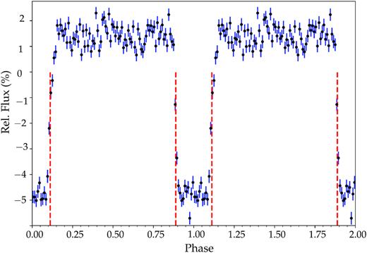
The phase folded and binned (into 100 bins) K2 light curve of WD1032 + 011 on a period of 0.092 d. The primary eclipse is clearly evident, and the red lines represent the 29.4-min cadence of the K2 data, showing the undersampling of the eclipse. The light curves have been duplicated over two periods for display purposes.
Position and magnitudes for WD1032 + 011.
| Property | Value | Survey |
|---|---|---|
| RA (J2000) | 10:34:48.93 | |
| Dec. (J2000) | + 00:52:01.4 | |
| Distance (pc) | 326.78 ± 36.92 | Gaia DR2 |
| FUV | 22.670 ± 0.224 | Galex |
| NUV | 20.152 ± 0.037 | Galex |
| u | 19.547 ± 0.032 | SDSS |
| g | 19.034 ± 0.010 | SDSS |
| r | 19.076 ± 0.012 | SDSS |
| i | 19.169 ± 0.019 | SDSS |
| z | 19.240 ± 0.076 | SDSS |
| Y | 18.820 ± 0.042 | UKIDSS LAS |
| J | 18.648 ± 0.056 | UKIDSS LAS |
| H | 18.202 ± 0.107 | UKIDSS LAS |
| K | 18.034 ± 0.141 | UKIDSS LAS |
2.2 FOcal Reducer and low-dispersion Spectrograph (FORS) spectroscopy
We observed WD1032 + 011 with the visual and near-ultraviolet FORS (Appenzeller et al. 1998) on the Very Large Telescope in service mode as part of programme 098.D-0717(A). We used the G1200B grism and the 1-arcsec slit to cover the majority of the Balmer lines including Hβ at a resolution λ/Δλ ∼ 1400. We obtained an hour of data on each of the nights of 2016 December 05, 06, and 24. Each hour was split into six exposures of 420 s, providing 18 spectra in total.
The data were reduced using the FORS specific reflex (Freudling et al. 2013) pipeline. The spectra were then normalized in molly and phase folded according to the ephemeris determined from the K2 data. The spectra clearly show that the white dwarf is moving on the orbital period determined from the K2 data, however, they are not of sufficient resolution to determine the systemic velocity, γ, or the radial velocity, K1, of the white dwarf and so were not included in the subsequent fitting presented here.
2.3 GMOS spectroscopy
As our FORS spectra were not of sufficient resolution to measure the radial velocity of the white dwarf, we observed WD1032 + 011 on the nights of 2019 January 11, 12, and 13 with the Gemini Multi-Object Spectrograph (GMOS: Hook et al. 2004) on Gemini-North in service mode as part of programme GN-2019A-Q-227 (PI: Debes). We obtained 24 spectra with the R831 grating with a central wavelength of 5750 Å; resulting in a wavelength range of 4600–6900 Å. We used the 0.75-arcsec slit, 2 × 2 binning and 900 s exposures to obtain a resolution of (λ/Δλ) ∼ 4000. The airmass was between 1 and 1.5 arcsec for the observations.
The data were reduced using the GMOS specific packages in iraf (Tody 1986) for long-slit spectra before being calibrated using a standard star observation of Hiltner 600.
2.4 GNIRS spectroscopy
We observed WD1032-011 with Gemini North and the cross-dispersed spectrograph GNIRS (Elias et al. 2006) as part of programme GN-2019A-Q-227 (PI: Debes). We used the short camera with the 1.00-arcsec slit providing a resolution of (λ/Δλ) ∼500 over the whole 0.8–2.5-μm spectrum. We nodded the observations with 440 s exposures taken at each nod point and combined the eight exposures at the reduction stage. The data were reduced using spextool v4.1 (Cushing, Vacca & Rayner 2004), which had been adapted for use with GNIRS (K. Allers, private communication) and telluric corrected using xtellcorr (Vacca, Cushing & Rayner 2003) and an A0V standard star.
2.5 McDonald 2.1-m Photometry
We acquired high-speed time-series photometry of WD1032 + 011 on four consecutive nights, 2017 December 18–21, using the Princeton Instruments ProEM frame-transfer CCD on the McDonald Observatory 2.1-m Otto Struve telescope. The nights were clear, with a new moon, but poor seeing. Each night we used an Astrodon Gen2 Sloan g′ filter, and in total our observations covered six eclipses of the white dwarf primary. See Table 2 for a summary of observing information and conditions.
McDonald 2.1-m observations of WD1032 + 011.
| Night | Filter | Seeing | Airmass | Exposure | Duration |
|---|---|---|---|---|---|
| (arcsec) | (s) | (h) | |||
| 2017 Dec 18 | g′ | 2.0 | 1.18−1.15 | 10 | 0.66 |
| 2017 Dec 19 | g′ | 2.3 | 1.31−1.20 | 10 | 2.93 |
| 2017 Dec 20 | g′ | 3.0 | 1.46−1.22 | 15 | 3.87 |
| 2017 Dec 21 | g′ | 3.6 | 1.41−1.25 | 15 | 3.83 |
Using standard calibration frames taken before each night of observation, we bias, dark, and flat-field corrected the McDonald images with iraf. We performed circular aperture photometry using the iraf routine ccd_hsp (Kanaan, Kepler & Winget 2002). Background counts were subtracted using an annulus placed around each aperture. We performed the aperture photometry both forward through each ingress and backward through each egress to ensure the aperture was properly placed on the centroid of our target as it went in and out of total eclipse.
To generate light curves for each night, we used the Wqed software suite (Thompson & Mullally 2013). We divided the target photometry by two nearby comparison stars, the same for each night, and then normalized by the target’s mean intensity. We clipped any outliers or heavily cloud-affected data from the light curves and then selected the optimal aperture size which minimized the average point-to-point scatter when out of eclipse. Lastly, we used Wqed to apply a barycentric correction to the mid-exposure time-stamp of each image.
2.6 ULTRACAM photometry
We observed three eclipses of WD1032 + 011 using ultracam (Dhillon et al. 2007) on the ESO New Technology Telescope. The observing information and conditions are listed in Table 3. ultracam observes in three filters simultaneously, with dead time of ∼25 ms, and we used on chip coadding in the u′ band to increase the exposure time to between 13.5 and 18 s, hence increasing the signal-to-noise ratio in this filter.
NTT/ultracam observations of WD1032 + 011.
| Night | Filters | Seeing | Airmass | Exposure |
|---|---|---|---|---|
| (arcmin) | (s) | |||
| 2018 Jan 19 | u′g′r′ | 1.4 | 1.24−1.36 | 6 |
| 2018 Jan 23 | u′g′r′ | 1.0 | 1.56−1.77 | 6 |
| 2019 Mar 01 | u′g′i′ | 0.7 | 1.41−1.49 | 4.5 |
| Night | Filters | Seeing | Airmass | Exposure |
|---|---|---|---|---|
| (arcmin) | (s) | |||
| 2018 Jan 19 | u′g′r′ | 1.4 | 1.24−1.36 | 6 |
| 2018 Jan 23 | u′g′r′ | 1.0 | 1.56−1.77 | 6 |
| 2019 Mar 01 | u′g′i′ | 0.7 | 1.41−1.49 | 4.5 |
The data were reduced using the ultracam pipeline software. The source flux was determined using aperture photometry with a variable aperture scaled according to the full width at half-maximum. Any variations in observing conditions were accounted for by determining the flux relative to a comparison star within the field of view.
We performed a fit to each light curve using lcurve (Copperwheat et al. 2010) to determine T0, and the continuum flux level, as the photometry on each night was performed using a different reference star.
3 RESULTS
3.1 Ephemeris
We used the initial ephemeris as determined from the K2 data, and fit each individual eclipse from the ULTRACAM and ProEM instruments in the g band with the light-curve fitting code lcurve (Copperwheat et al. 2010) to determine the centre of each eclipse. We selected an eclipse that lay in the middle of the observed times to represent cycle 0 (the first eclipse on the 2017 December 21), and determined the cycle of each eclipse using the K2 period, before fitting the function T = T0 + E*P, where T is time of eclipse, E is the cycle number and T0 and P are the zero-point and period, respectively, to the data. The linear ephemeris was fit using the affine-invariant Markov chain Monte Carlo (MCMC) sampler emcee (Foreman-Mackey et al. 2013). The cycle numbers were adjusted to minimize the covariance between T0 and P. The final ephemeris is given in Table 4. The best fit has a χ2 of 3.9 with 7 degrees of freedom. The individual eclipse times, including the uncertainties, are given in the Appendix (Table A1).
Final system parameters for WD1032 + 011.
| Parameter | Value | Info |
|---|---|---|
| WD Teff(K) | 9950 ± 150 | SED |
| WD log g | 7.65 ± 0.13 | SED |
| E(B − V) | 0.03 ± 0.01 | SED |
| Cooling time (Gyr) | 0.455 ± 0.080 | FORS |
| T0 (BMJD) | 58381.2439008(10) | ultracam, ProEM |
| P (d) | 0.09155899610(45) | ultracam, ProEM |
| γ1 (kms−1) | 122.08 ± 1.94 | GMOS |
| K1 (kms−1) | 48.8 ± 2.64 | GMOS |
| Inclination (°) | 87.5 ± 1.4 | ultracam |
| R1 (R⊙) | 0.0147 ± 0.0013 | ultracam |
| R2 (R⊙) | 0.1052 ± 0.0101 | ultracam |
| M1 (M⊙) | 0.4502 ± 0.0500 | SED |
| M2 (M⊙) | 0.0665 ± 0.0061 | ultracam |
| a(R⊙) | 0.6854 ± 0.0244 | ultracam |
3.2 Radial velocity
The GMOS spectra were analysed using the molly software1 package. We analysed the spectra using the techniques described by Parsons et al. (2017), fitting the orbit using all of the spectra, not determining velocities for each individual spectrum. We normalized the spectra by dividing by the average spectrum for each hour-long observing block, phase folded the spectra using the ephemeris derived from the eclipses (in the previous subsection), and fitted the Hβ absorption line using three Gaussians, two broad and one narrow. The three Gaussians were fixed to have the same K and γ velocities, and were allowed to vary around the orbit as γ1 + K1sin (2πϕ), where ϕ is the orbital phase. The errors on the radial velocity parameters were determined by adding 1 kms−1 in quadrature in order to achieve a reduced chi-squared of |$\chi _{\nu }^2\sim$| 1. The final velocities were K1 = 48.8 ± 2.6 kms−1 and γ = 122.1 ± 1.9 kms−1. The trailed spectra and model are shown in Fig. 2.
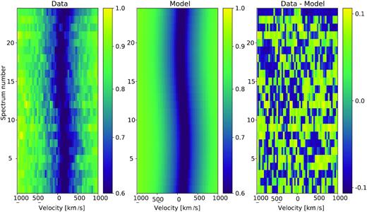
Trailed GMOS spectra showing one full orbit, centred on the Hβ line shown with the data (left-hand panel), model generated from the Gaussian fitting (centre panel), and the fit residuals (right-hand panel).
We also searched the spectra for any other emission or absorption lines that may have been in our wavelength range, notably Na I and Mg I, but none were present.
3.3 Effective temperature and log g
We combined all 18 of the FORS spectra by shifting them into the rest frame of the white dwarf using the K1 value from the radial velocity fitting, and then used DA white dwarf models from Koester (2010) to determine the effective temperature and gravity of the white dwarf. Our model grid consists of a set of DA white dwarf model spectra with mixing length ML2/α = 0.8 computed on a grid of 6.5 ≥ log g ≥ 9.5 in steps of 0.25 dex and 6000 ≥ Teff ≥ 40000 K in steps of 1000 K. Our parameters have errors that are underestimated as suggested by Napiwotzki, Green & Saffer (1999) so we follow their method and assume an uncertainty of 2.3 per cent in Teff and 0.07 dex in log g. The new parameters are Teff = 10196 ± 235 K and log g = 7.81 ± 0.07 (Fig. 3). These values have a much lower log g compared to the Eisenstein et al. (2006) values. However, they still predict a white dwarf far more luminous than the Gaia parallax implies (such a white dwarf would be expected to have an absolute magnitude of MG = 9.3 compared to the actual value of MG = 11.8, (Gaia Collaboration et al. 2018)). We decided to independently measure the white dwarf parameters by fitting the spectral energy distribution (SED) of WD1032 + 011 with white dwarf models, including the Gaia parallax information within the fit.
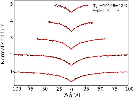
Combined FORS2 spectrum (black, Hβ to H8, bottom to top panel) of WD1032 + 011 with the best-fitting model Teff = 10196 ± 72 K and log g = 7.81 ± 0.02 overplotted in red. These errors are the fitting errors only. Please see the main text for an explanation of the likely true errors.
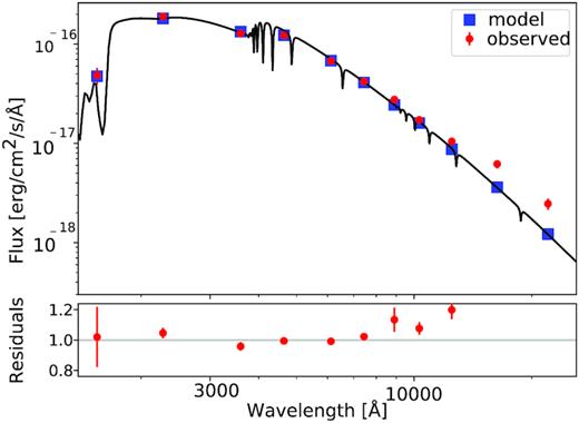
SED of WD1032 + 011 (red points are GALEX, SDSS, and UKIDSS measurements) with the best-fitting model white dwarf spectrum (black line and blue points). Only measurements blueward of the z band were included in the fit. The lower panel shows the residuals to the fit, which rise rapidly at longer wavelengths where the contribution from the brown dwarf is no longer negligible. The final parameters from this fit are Teff = 9950 ± 150 K and log g = 7.65 ± 0.13.
We retrieved broad-band photometry of WD1032 + 011 from GALEX, SDSS, and UKIDSS (see Table 1) and fitted these with DA white dwarf spectra from Koester (2010). For a given combination of log g and Teff, we used the mass–radius relation of Panei et al. (2007) for He core white dwarfs to estimate the white dwarf radius, which, combined with the parallax, was used to scale the model spectrum. We also included the effects of reddening. We discarded the z-, Y-, J-, H- and K-band measurements since the brown dwarf contributes a non-negligible amount of flux at these wavelengths. Model parameters and their uncertainties were found using the MCMC method (Press et al. 2007) implemented using the python package emcee (Foreman-Mackey et al. 2013), where the likelihood of accepting a model was based on a combination of the χ2 of the SED fit and prior probabilities on the parallax (Gaussian, based on the Gaia measurement and associated uncertainty) and the reddening (uniform from zero up to the maximum possible value of 0.052 based on reddening maps, Schlafly & Finkbeiner 2011). The final parameters are listed in Table 4 and are consistent with the values from the fit to the FORS2 spectrum but with a slightly lower surface gravity (thus lower mass). The somewhat larger log g implied from the spectral fit may be due to some minor contamination of the Balmer lines by emission from the brown dwarf, although there is no clear evidence of emission lines in the FORS2 spectra.
3.4 Spectral type of the secondary
To determine the spectral type of the brown dwarf secondary we created combined white dwarf-brown dwarf models. We used a white dwarf model from Koester (2010) using our derived Teff and log g and the model absolute magnitudes of a lone white dwarf with these parameters from Holberg & Bergeron (2006) and Tremblay, Bergeron & Gianninas (2011) to create a normalized white dwarf model at 10 pc. We then repeated this process using the absolute magnitudes of brown dwarfs with spectral types L3, L4, L5, and L6 from Dupuy & Liu (2012) and brown dwarf template spectra from Cushing, Rayner & Vacca (2005) and Rayner, Cushing & Vacca (2009) archived in the IRTF spectral library. Ensuring both sets of spectra were on the same wavelength scale, we then combined them, and normalized the models to the SDSS i band, where the brown dwarf contribution to the total flux is negligible, as can be seen from the SED fitting to the white dwarf photometry.
The GNIRS spectrum, templates, and UKIDSS magnitudes are consistent with the L4–L6 spectral type suggested by Steele et al. (2011) once the 30 per cent rms scatter in the absolute magnitudes from Dupuy & Liu (2012) is taken into account. Overall, a brown dwarf with a spectral type of L5 is the most likely companion, although spectral types of L4 and L6 cannot be completely ruled out (Fig. 5).
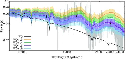
The GNIRS spectrum (grey) shown with the model white dwarf (black), and model white dwarf−brown dwarf spectra (orange, green, purple, blue). The UKIDSS photometry are also displayed. The shaded, coloured regions represent the 30 per cent rms scatter on the spectral types derived from the absolute magnitudes in Dupuy & Liu (2012).
3.5 Masses and radii
We normalized the ultracam light curves to have a continuum level of 1, and phase folded using the ephemeris derived above in Section 3.1. We then fitted the ultracam light curves using the method described in Littlefair et al. (2014) using an affine-invariant MCMC sampler (emcee; Foreman-Mackey et al. 2013) and the light-curve fitting code lcurve (Copperwheat et al. 2010). We used 100 walkers, with a burn-in period of 300, and 300 production steps. We used our parameters of the white dwarf and the Steele et al. (2011) parameters for the brown dwarf to find the quadratic limb-darkening coefficients with Teff = 9950 K, log g = 7.65 from Gianninas et al. (2013) for the white dwarf and Teff = 1700 K, log g = 5.0 from Claret, Hauschildt & Witte (2012) for the brown dwarf. We only used the ultracam data for this fitting as it has the highest cadence and smallest scatter which is needed to properly fit the ingress and egress of the eclipses.
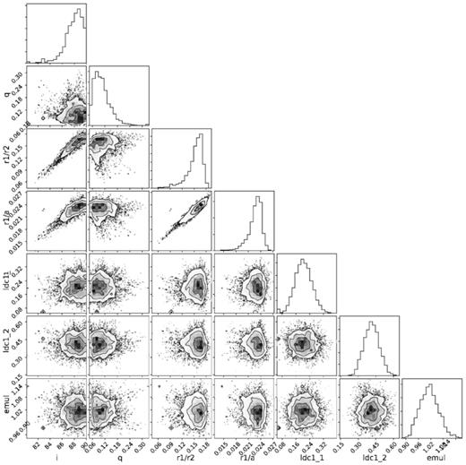
We allowed the mass ratio (q), radii (R1/a, R2/a), inclination (i), and the quadratic limb-darkening parameters to vary. We put priors on the limb-darkening parameters using a Gaussian distribution with twice the standard deviation suggested from the SED fit and the limb-darkening tables relevant to each star. A half-Gaussian prior was also used for the mass ratio, conservatively set with a mean of 0 and a standard deviation of 0.3 using the white dwarf mass derived from the SED and a brown dwarf mass from the Baraffe et al. (2003) models for spectral type L5 (see the previous section). Uniform priors were used for the radii and inclination. The acceptance fractions were 53 per cent for the g band, 51 per cent in the u band, and 51 per cent in the r band.
From the mass of the white dwarf, the orbital period and the radial velocity of the white dwarf, we construct the mass function, and combine with the inclination from the light-curve fit to find the brown dwarf mass and the orbital separation, which follows from Kepler’s law. The separation is used to rescale the radii from the light curve fits to give the final parameters of the system, which can be found in Table 4, with the final fits shown in Fig. 6. The corner plots for the fits are given in Appendix B. The mass and radius we derive for the white dwarf are consistent with both He and CO-core white dwarf models, but agree best with a CO model with a thin (10–10 M⊙) envelope.
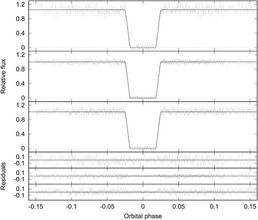
u′ (top panel), g′ (middle panel), and r′ (bottom panel) light curves from all three nights of ULTRACAM data, with the best-fitting model and residuals in each band. The out of eclipse flux was normalized to 1.
The constraint on the inclination from a single eclipse light curve is subtle. The ingress and egress duration depend upon the inclination, but are highly degenerate with the radii of the two components. Small changes in the shape of the ingress and egress can break this degeneracy, but the shape is also dependent on the limb darkening of the white dwarf. This can make convergence difficult, and raise doubts about the constraint on the inclination from a primary eclipse alone. We checked against convergence issues by re-fitting the primary eclipse using a different parametrization. We allowed the mid-eclipse time T0 to be a free parameter and parameterized the eclipse using the mass of the white dwarf, temperature of the white dwarf, the radius of the white dwarf and the radius ratio of the binary. At each step in the MCMC chain, we calculate the relevant limb-darkening coefficients from the white dwarf temperature and the tables of Gianninas et al. (2013). We also checked our convergence by running the fits from different starting points, and by using both a quadratic and a Claret limb-darkening law. All fits were consistent and gave posterior estimates of the brown dwarf mass and radius of M2 = 0.066 ± 0.005 M⊙ and R2 = 0.099 ± 0.003R⊙, which is consistent with our original determination. The only main difference is that this parametrization cannot rule out an inclination of 90° for the binary, which is probably due to the relaxed constraint on T0.
4 DISCUSSION
In order to constrain the age of WD1032 + 011, we have performed a kinematic analysis using the proper motions from Gaia and our measured velocities. The cooling age of the white dwarf from the Panei et al. (2007) models is 800 Myr, so this gives us the minimum age of the system. We calculate the UVW space motions with respect to the local standard of rest to be, U = −163 ± 19 km s−1, V = −73 ± 2 km s−1, and W = 37 ± 8 km s−1 (where U is positive towards the Galactic centre). Using the same method we used in Littlefair et al. (2014) and the membership probabilities in Bensby, Feltzing & Oey (2014) for memberships of the thin disc, thick disc and halo, we determine that WD1032 + 011 is 130 times more likely to belong to the thick disc than the halo, and 20 000 times more likely to belong to the thick disc than the thin disc. Hence WD1032 + 011 is likely to belong to the thick disc but we cannot entirely rule out halo membership. This result means that the system is probably old, with a likely age of ∼10 Gyr if a member of the thick disc (Kilic et al. 2019). Gallart et al. (2019) show that for the kinematics of WD1032 + 011 and any radial velocity between −120 to +120 km s−1 (γ = 122.08 ± 1.94 km s−1) thick disc membership is favoured, strongly suggesting an age greater than 5 Gyr and a moderately low metallicity of [Fe/H]∼−0.3.
With the 5−10 Gyr age estimate from the kinematic analysis, we can compare our brown dwarf mass and radius to the low-metallicity ([Fe/H] = –0.5) Sonora–Bobcat models. Using these models. a 10-Gyr old 0.066 M⊙ brown dwarf would have Teff = 988 K and a radius of 0.079 R⊙. Similarly, a 6-Gyr old 0.066 M⊙ brown dwarf would have Teff = 1163 K and a radius of 0.079R⊙. These models suggest that WD1032 + 011 should have a much smaller radius than the one we measure here (0.1052 ± 0.0101R⊙). The effective temperatures are also much lower than one would expect for an L5 dwarf. A 1500 K (approximate effective temperature of an L5 dwarf) 0.066 M⊙ brown dwarf would have an age of only 2 Gyr according to the Sonora–Bobcat models, but should also have a radius of 0.0851R⊙, again smaller than our measured radius. It is possible that the system has an age of 2 Gyr, but this would be unusually young for a thick disc member. We therefore conclude that WD1032 + 011 is likely hotter and larger than the models predict, making it the first inflated brown dwarf to be discovered orbiting a white dwarf.
WD1032 + 011 is only the third white dwarf-brown dwarf binary where the radius of the brown dwarf can be directly measured (Table 5). Both the previously known eclipsing brown dwarfs, SDSS J141126.20 + 200911.1, and SDSS J120515.80 − 024222.6, show no inflation and are consistent with the 6–10 Gyr Sonora–Bobcat isochrones from Marley et al. (2018) (Fig. 7). WD1032 + 011 is the first brown dwarf in a white dwarf-brown dwarf binary to have been shown to be inflated, which is extremely interesting as the mechanism causing the inflation is unknown. SDSS J120515.80 − 024222.6 has a much hotter white dwarf primary, and a much shorter orbital separation than WD1032 + 011 yet is not inflated, indicating that any inflation cannot be due to irradiation alone. We also do not see any signs of interaction between the white dwarf and brown dwarf in WD1032 + 011 as is seen for NLTT5306AB (Longstaff et al. 2019) where the white dwarf shows emission features due to weak accretion from the brown dwarf, possibly due to a wind.
![Masses and radii for all brown dwarfs transiting white dwarfs (filled squares; Littlefair et al. 2014; Parsons et al. 2017), and main-sequence stars (Carmichael et al. 2020 and references therein). WD1032 is marked with a filled triangle. Also shown are the Sonora–Bobcat evolutionary models of Marley et al. (2018) for 100 Myr, 600 Myr, 2 Gyr, 6 Gyr, and 10 Gyr with solar metallicity (grey) and low-metallicity ([Fe/H] = −0.5) models for 2, 6, and 10 Gyr (black).](https://oup.silverchair-cdn.com/oup/backfile/Content_public/Journal/mnras/497/3/10.1093_mnras_staa1608/1/m_staa1608fig7.jpeg?Expires=1750537542&Signature=qfsQtmePS11G55-Zz-Kh9L8RF4VDyf35cqo4jjgSNu8NUyiIvPyStQMI1bBpyheWJjBpeDfnyIaI1Im6yANJNc8vKX7bHpEikIpUV6Of-lW~BH1amJ315DxGpM1DLSIC~OkwNX4ivXSTN2PHJUuIETxYxEOb91isiv-VWxmItckDQtZ1lk0oDlu1tkTkN5uo0rDnjf6B-Qm3HYdfJTHeGYkCxvqu7C~f3taRkwanHgESmO3c12wUb-MdiqqmSWktSSKBH86xkOSasLourFFQsC3IacrPoWLfP24vxlmWxhwbg0vz0XGJI5bX58PCfnSbvt3qdvWMuilNZayasNZe2A__&Key-Pair-Id=APKAIE5G5CRDK6RD3PGA)
Masses and radii for all brown dwarfs transiting white dwarfs (filled squares; Littlefair et al. 2014; Parsons et al. 2017), and main-sequence stars (Carmichael et al. 2020 and references therein). WD1032 is marked with a filled triangle. Also shown are the Sonora–Bobcat evolutionary models of Marley et al. (2018) for 100 Myr, 600 Myr, 2 Gyr, 6 Gyr, and 10 Gyr with solar metallicity (grey) and low-metallicity ([Fe/H] = −0.5) models for 2, 6, and 10 Gyr (black).
| Name | Period | M1 | R1 | Teff | M2 | R2 | Spectral type |
|---|---|---|---|---|---|---|---|
| (h) | (M⊙) | (R⊙) | (K) | (M⊙) | (R⊙) | ||
| WD1032 + 011 | 2.20 | 0.450 ± 0.050 | 0.0148 ± 0.0013 | 9950 ± 150 | 0.067 ± 0.006 | 0.105 ± 0.010 | L5 |
| SDSS J141126.20 + 200911.1 | 2.03 | 0.53 ± 0.03 | 0.0142 ± 0.0006 | 13000 ± 300 | 0.050 ± 0.002 | 0.072 ± 0.004 | T5 |
| SDSS J120515.80 − 024222.6 | 1.19 | 0.39 ± 0.02 | 0.0217–0.0223 | 23680 ± 430 | 0.049 ± 0.006 | 0.081–0.087 | >L0 |
There are also four brown dwarfs known to be eclipsing hot sdB stars (Geier et al. 2011; Schaffenroth et al. 2014, 2015). It is, however, challenging to determine the mass and radius of hot subdwarfs as they are often pulsating and there is no well-defined mass–radius relationship as there is for white dwarfs. Large uncertainties regarding the mass and radius of the primary can cause large errors on measurements of the brown dwarf, meaning radii from mass–radius relations are often adopted. For this reason, we do not discuss brown dwarfs in binaries with hot subdwarfs further here. There are, however, ∼20 systems where a brown dwarf eclipses a main-sequence star. These systems have been discovered through transiting planet searches, and do have reliable masses for the primary stars. The mass–radius relationship for all 23 transiting, irradiated brown dwarfs is shown in Fig. 7.
When we compare the three brown dwarfs orbiting white dwarfs (filled boxes and circle in Fig. 7) to the population of irradiated brown dwarfs orbiting main-sequence stars it is clear that most, if not all, of the low-mass objects (M ≲ 35MJup) are inflated. None of these brown dwarfs orbit a star that has been identified as younger than 1 Gyr, as the radii of the brown dwarf would suggest. At masses greater than 35MJup, the majority of objects sit on the 5–10-Gyr isochrone. The exceptions are NGTS-7Ab (Jackman et al. 2019; |$M=75.5^{+3}_{-13.7}$|MJup), which is ∼ 55 Myr old, hence its position near, but below the 100-Myr isochrone; TOI0-503 (Šubjak et al. 2019; M = 53.7 ± 1.2MJup) which is 180 Myr old and has a radius consistent with this; KOI-189b, which may, in fact, be a low-mass star (Díaz et al. 2014; M = 78 ± 3.4MJup), and may be slightly inflated, as age estimates for this system are ∼5 Gyr. However, inflated late M-dwarf radii are not uncommon, and are often attributed to convection within the star being inhibited due to magnetic fields (e.g. MacDonald & Mullan 2014). The remaining two objects that do not sit on the 5–10-Gyr isochrones are CoRoT-33b (Csizmadia et al. 2015) and CoRot-15b (Bouchy et al. 2011). Both of these objects have large uncertainties on their radii, but also orbit active stars which may have had some effect on the measurement of the radius of the brown dwarf.
Parsons et al. (2018) found that the scatter in the M-dwarf mass–radius relationship was 6.2 ± 4.8 per cent, with only about a quarter of M dwarfs being consistent with models. They determined that there was no trend with either age or metallicity as to which M-dwarfs are inflated. It may be that a similar relationship, with similar scatter exists as we move into the brown dwarf regime, particularly for the higher mass brown dwarfs.
5 CONCLUSIONS
We have discovered a new eclipsing, detached short-period white dwarf-brown dwarf binary member of the thick disc. Our multicolour light curves of the eclipses show that the brown dwarf is inflated when compared to metal-poor evolutionary models. A Gemini GNIRS NIR spectrum of the brown dwarf is consistent with a spectral type of L5, which would suggest an effective temperature hotter than predicted by the models for the age of the thick disc.
ACKNOWLEDGEMENTS
We thank the GMOS team at Gemini-North, in particular, Sandy Leggett, Siyi Xu, and André-Nicolas Chené for their assistance and advice with the scheduling and data reduction.
SLCl and SGP acknowledge support from STFC Ernest Rutherford Fellowships and IPB acknowledges support from the University of Leicester College of Science and Engineering. SGP also acknowledges the support of the Leverhulme Trust. VSD and ultracam are supported by the STFC grant SST/R000964/1. DW and KW acknowledge support from NSF Grant 1707419. Partial support for this work was also provided by NASA K2 Cycle 6 grant 80NSSC19K0162.
This work is based on observations obtained at the Gemini Observatory, which is operated by the Association of Universities for Research in Astronomy, Inc., under a cooperative agreement with the NSF on behalf of the Gemini partnership: the National Science Foundation (United States), National Research Council (Canada), CONICYT (Chile), Ministerio de Ciencia, Tecnología e Innovación Productiva (Argentina), Ministério da Ciência, Tecnologia e Inovação (Brazil), and Korea Astronomy and Space Science Institute (Republic of Korea). Also based on observations collected at the European Organisation for Astronomical Research in the Southern Hemisphere under ESO programme 098.D-0717(A). This research is based on observations made with the Galex mission, obtained from the MAST data archive at the Space Telescope Science Institute, which is operated by the Association of Universities for Research in Astronomy, Inc., under NASA contract NAS 5-26555.
Footnotes
REFERENCES
APPENDIX A: ECLIPSE TIMES
Eclipse times of WD1032 + 011.
| Date | BMJD (TDB) | Eclipse number | O – C (s) | Instrument |
|---|---|---|---|---|
| 2017 Dec 18 | 58105.468197(16) | –3012 | -0.6 | ProEM |
| 2017 Dec 19 | 58106.4753509(54) | –3001 | -0.2 | ProEM |
| 2017 Dec 20 | 58107.390991(32) | –2991 | 4.0 | ProEM |
| 2017 Dec 20 | 58107.482501(15) | –2990 | –0.2 | ProEM |
| 2017 Dec 21 | 58108.398083(14) | –2980 | –0.9 | ProEM |
| 2017 Dec 21 | 58108.489669(21) | –2979 | 1.5 | ProEM |
| 2018 Jan 19 | 58137.2391769(33) | –2665 | 0.06 | ultracam |
| 2018 Jan 23 | 58141.1762135(35) | –2622 | 0.03 | ultracam |
| 2019 Mar 1 | 58543.3033239(17) | 1770 | -0.02 | ultracam |
APPENDIX B: CORNERPLOTS
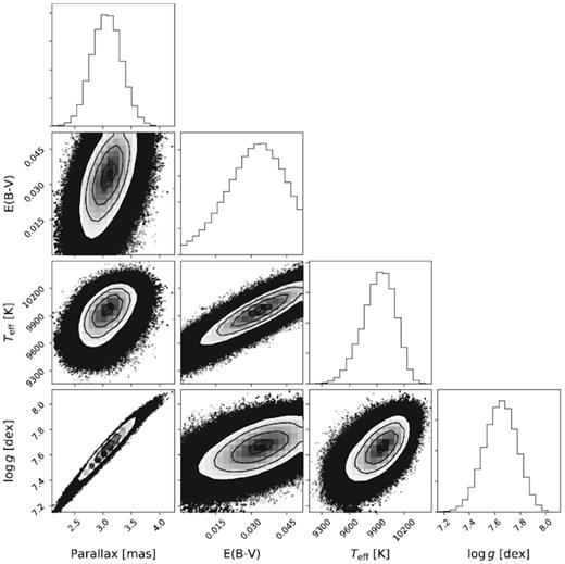
Corner plot from the MCMC output used to fit the SED of the white dwarf.
Corner plot from the MCMC output used to fit the u-band light curve.
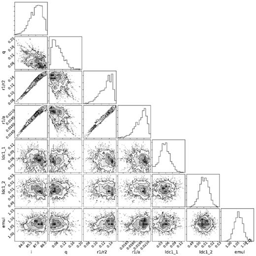
Corner plot from the MCMC output used to fit the g-band light curve.
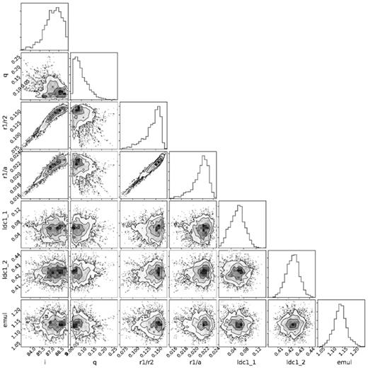
Corner plot from the MCMC output used to fit the r-band light curve.
Author notes
STFC Ernest Rutherford Fellow.
