


ABSTRACT
We present the galaxy group catalogue for the recently completed 2MASS Redshift Survey (2MRS; Macri et al. 2019) which consists of 44 572 redshifts, including 1041 new measurements for galaxies mostly located within the Zone of Avoidance. The galaxy group catalogue is generated by using a novel, graph-theory based, modified version of the friends-of-friends algorithm. Several graph-theory examples are presented throughout this paper, including a new method for identifying substructures within groups. The results and graph-theory methods have been thoroughly interrogated against previous 2MRS group catalogues and a Theoretical Astrophysical Observatory (TAO) mock by making use of cutting-edge visualization techniques including immersive facilities, a digital planetarium, and virtual reality. This has resulted in a stable and robust catalogue with on-sky positions and line-of-sight distances within 0.5 and 2 Mpc, respectively, and has recovered all major groups and clusters. The final catalogue consists of 3022 groups, resulting in the most complete ‘whole-sky’ galaxy group catalogue to date. We determine the 3D positions of these groups, as well as their luminosity and comoving distances, observed and corrected number of members, richness metric, velocity dispersion, and estimates of R200 and M200. We present three additional data products, i.e. the 2MRS galaxies found in groups, a catalogue of subgroups, and a catalogue of 687 new group candidates with no counterparts in previous 2MRS-based analyses.
1 INTRODUCTION
Galaxies are not isolated in space. They form part of larger structures such as groups, clusters, filaments, and voids that together compose the so-called cosmic web (Davis et al. 1982; Zeldovich, Einasto & Shandarin 1982; Klypin & Shandarin 1993; Bond, Kofman & Pogosyan 1996; Jarrett 2004). These large-scale structures are immediately revealed when visually examining the distributions of galaxy positions in redshift space (Peebles 1980; Huchra & Geller 1982; Tully & Fisher 1987; Peebles 1993; Fairall 1998; Huchra et al. 2005; Crook et al. 2007; Robotham et al. 2011; Huchra et al. 2012; Tempel et al. 2016, 2018). However, visually identifying and classifying structures is a subjective method that is neither robust nor quantitative (Crook et al. 2007; Robotham et al. 2011; Huchra et al. 2012; Alpaslan et al. 2014; Saulder et al. 2016; Jarrett et al. 2017; Kourkchi & Tully 2017). As a result, several algorithmic and computational methods for identifying large-scale structure have been put forward. One of the most established and applied methods over the past decades has been the Friends-of-Friends (FoF) algorithm (Huchra & Geller 1982), which has been extensively used to find galaxy groups in numerous magnitude-limited redshift surveys (Huchra & Geller 1982; Ramella, Pisani & Geller 1997; Trasarti-Battistoni, Invernizzi & Bonometto 1997; Crook et al. 2007; Robotham et al. 2011).
Redshift surveys provide one of the most convenient and efficient tools to study the three-dimensional distribution of galaxies. Being able to objectively identify large-scale structures within these surveys is relevant to addressing a number of unanswered questions in observational cosmology related to the cosmic microwave background (CMB) dipole anisotropy (Rauzy & Gurzadyan 1998; Bilicki et al. 2011), establishing a relationship between galaxies and dark matter haloes and probing dark matter interactions (Coutinho 2016; Lu et al. 2016), constraining cosmological models (Peebles 1980), and exploring the effect of environment on galaxy evolution (Dressler 1980; Tempel et al. 2016, 2018). Redshift surveys come in a variety of flavours; the two most common ones are those constrained to a small solid angle on the sky and targeting galaxies at high redshifts (so-called pencil beam surveys), and those covering larger fractions of the sky at the expense of depth. The exact nature of the redshift survey depends on the science goals at hand, instrumentation, and availability of telescope time (Fairall 1998). Although numerous large-area redshift surveys have been made over the decades, none span the entire 4|$\pi$| sr of the sky. The overwhelming majority of so-called whole-sky surveys exclude the regions close to the plane of the Milky Way where high stellar densities, an increasingly brighter background, and high levels of extinction make observing galaxies very difficult (Saunders et al. 2000; Kraan-Korteweg et al. 2018). This region of exclusion is often referred to as the Zone of Avoidance (ZoA).
As a result of the ZoA, a truly ‘whole-sky’ redshift survey does not exist. The requirement for such a survey has been highlighted for several decades to fully explain the CMB dipole anisotropy, a well-known signature caused by the peculiar motion of the Milky Way (Lineweaver et al. 1996; Rauzy & Gurzadyan 1998). This motion cannot adequately be accounted for due to the obscuration by the ZoA of large mass concentrations such as the Great Attractor (Lynden-Bell et al. 1988; Kraan-Korteweg & Lahav 2000) and the recently discovered Vela Supercluster (Kraan-Korteweg et al. 2015, 2017; Courtois et al. 2019). While a truly whole-sky magnitude-limited redshift survey does not exist, imaging surveys have been made of the entire sky. Notably among these is the 2 Micron All Sky Survey (2MASS), which uniformly mapped 99.998|${{\ \rm per\ cent}}$| of the sky in the J, H, and Ks bands. Near-infrared light is far less affected by dust in the Galactic plane, resulting in a less-prominent ZoA in 2MASS. The 2MASS extended source catalogue (2MASX; Jarrett 2004; Skrutskie et al. 2006) contains ∼1.6 million sources with |$K_{\rm s}^{\rm o}\lt 13 {_{.}^{\rm m}}5$| and is the most complete all-sky galaxy catalogue to date. However, the sheer number density of stars in the Galactic plane makes 2MASX incomplete below |b| ∼ 5–8○ depending on Galactic longitude (Jarrett et al. 2000).
The whole-sky nature (and diminished ZoA impact) of 2MASX enabled the 2MASS Redshift Survey (2MRS; Huchra et al. 2005, 2012; Macri et al. 2019), a 20-yr concerted effort to measure the redshifts of all ∼45000 2MASX sources with |$K^{\rm o}_{\rm s} \lt 11{_{.}^{\rm m}}75$| and thus obtain the most comprehensive (coverage-wise) whole-sky redshift survey to date. A preliminary data release with a magnitude limit of |$K^{\rm o}_{\rm s} \lt 11{_{.}^{\rm m}}25$| consisted of ∼24 000 galaxies (Huchra et al. 2005). The initial data release that reached the target magnitude depth contained over 44 000 galaxies (Huchra et al. 2012), but was still significantly incomplete at low Galactic latitudes; the final data release (Macri et al. 2019) added the remaining ∼1000 redshifts, mostly in the ZoA. Fig. 1 shows the distribution of measurements from the two latter papers. The recent completion of 2MRS, with most of the new redshifts lying close to the ZoA, allows for new large-scale structures in this thinly mapped area to be uncovered.

A further benefit of having a complete whole-sky galaxy catalogue covering the local Universe is that it lends itself well to the derivation of a group catalogue, one that is more complete along the ZoA than previous work. These catalogues can be complementary to dedicated surveys within the ZoA (e.g. Ramatsoku et al. 2016; Staveley-Smith et al. 2016; Kraan-Korteweg et al. 2018). A complete whole-sky local Universe group catalogue is also required to quantify other large-scale structures such as filaments and voids (Alpaslan et al. 2014), which are useful in conjunction with other studies of galaxy flows due to large-scale structures in the local Universe (Pomarède et al. 2017; Courtois et al. 2019; Tully et al. 2019). Furthermore, a complete 2MRS group catalogue based on spectroscopic redshifts can be compared to one based on photometric redshift estimates (2MPZ; Bilicki et al. 2014), which may improve the accuracy of the latter technique.
In order to characterize the large-scale structure revealed by these new redshifts we have modified the FoF algorithm and, after optimization, applied it to the final (deepest and complete) version of 2MRS. This modified version of the FoF algorithm aims to improve upon the already successful traditional one by addressing several shortcomings such as sensitivity to initial conditions, non-generalizable parameter selection, and non-physical group membership identification. In this paper, we present an FoF-based group finder resulting in what we believe to be a highly accurate and robust ‘whole-sky’ galaxy group catalogue. We verified our results by comparing them against previous galaxy catalogues based on earlier versions of 2MRS and a deep mock catalogue to test for various (Malmquist-like) biases in the algorithm, and by performing an exhaustive visual inspection using state-of-the-art 3D visualization tools.
Galaxies are not homogeneous in their physical make-up. They come in numerous shapes, sizes, masses, morphologies, and chemical make-up (Buta 2013; Jarrett et al. 2017). How galaxies form, evolve, build their stellar populations, and form their distinct morphologies presents many challenges to our understanding of the Universe. It is widely agreed that the effect of environment on the make-up of a galaxy is significant (Dressler 1980; Gordon et al. 2018; Bianconi et al. 2020; Carlesi et al. 2020; Otter et al. 2020). Studying the role that environment has on galaxy formation and evolution requires knowledge not only of the positions of the galaxies (which act as tracers of the baryonic mass throughout the cosmic web) but also of the environments in which these galaxies find themselves. Thus, redshift surveys and their corresponding galaxy group catalogues make for very important tools in decoding galaxy formation and evolution (Dressler 1980; Fairall 1998; Alpaslan et al. 2014; Jarrett et al. 2017).
As has been previously mentioned there are two main types of redshift surveys, namely very narrow and deep surveys and wide and shallow surveys. Narrow surveys are excellent tools for studying galaxy evolution and formation through cosmic time while shallow surveys lend themselves very well to exploring the role of environment on galaxy morphology in the Local Universe (z < 0.2). Nearby galaxies in the local Universe are most often found in galaxy groups (van de Weygaert & Bond 2008; Robotham et al. 2011; Gordon et al. 2018). Thus, the 2MRS galaxy group catalogue (being the widest area survey to date) makes for an optimal survey to explore the effects of galaxy environments ranging from small groups (e.g. Local Group) to the largest of clusters (e.g. Coma Cluster); previous 2MRS group catalogues have been successfully applied to environmental studies of galaxies (e.g. O’Brien et al. 2018; Calderon & Berlind 2019; Greene et al. 2019).
The remainder of this paper is laid out as follows: we describe our method of identifying groups in the 2MRS in Section 2, including the modifications we have made to the FoF algorithm. The numerous visualization techniques thate used to interrogate our methods are discussed in Section 3. The final 2MRS catalogue as well as supplementary catalogues are presented in Section 4. Discussions and conclusions can be found in Section 5. Throughout this paper we adopt H0 = 73 km s−1 Mpc−1, ΩM = 0.3, and ΩΛ = 0.7.
2 GROUP FINDER
2.1 Friends-of-Friends
The FoF algorithm has been the canonical method for identifying groups in magnitude-limited redshift-surveys because of its simplicity (Huchra & Geller 1982; Ramella et al. 1997; Crook et al. 2007; Duarte & Mamon 2014; Tully 2015; Tempel et al. 2016). Although the core algorithm remains, for the most part, unchanged from the original formalism by Huchra & Geller (1982), its subsequent applications to various redshifts surveys have varied according to their wavelength coverage, completeness, depth, and area.
We based our FoF algorithm for the |$K^{\rm o}_{\rm s}\lt $|11|${_{.}^{\rm m}}$|75 2MRS sample on the one developed by Crook et al. (2007), who created a group catalogue based on the 2MRS |$K^{\rm o}_{\rm s}\lt 11{_{.}^{\rm m}}25$| sample (Huchra et al. 2005). In its simplest form, this algorithm iteratively isolates galaxies i and j and determines whether they are in close enough proximity to each other in projected spatial and radial velocity-space to be gravitationally associated. If i and j are close in redshift space they are considered ‘friends’. All friends of i can be found this way, followed by all the friends of friends of i, and so forth. A group is then defined according to degrees of association.
In principle, we want galaxies to be considered ‘friends’ if they are gravitationally bound. If the projected separation of galaxy i and galaxy j, with an angular separation θij, defined as |$D_{ij}=\sin (\frac{\theta _{ij}}{2})\frac{v_{\text{avg}}}{H_0}$|, is less than some linking length Dl, we know that they are close enough, in terms of a plane-of-sky projection, to be associated.
We also consider the line-of-sight distance, represented in this case by the difference in cz between the two galaxies (Δv = |vi − vj|). If this value is smaller than some linking velocity vl, the galaxies are close enough to be associated along the line of sight.
If a pair of galaxies meets both conditions (associated both along the plane of sky and line of sight), we consider them ‘friends’. The two parameters used to determine whether two galaxies are friends are Dl and vl.
The fiducial velocity vf is set to 103 km s−1, following Crook et al. (2007). This value was carefully determined in Huchra & Geller (1982) by evaluating the probable number of interlopers as a result of the chosen value using the methods presented in Davis et al. (1982). This particular value has been thoroughly verified by Geller & Huchra (1983), Ramella, Geller & Huchra (1989), and Ramella et al. (1997).
Defining the linking length Dl according to equation (1) scales the surveyed volume by the number density of galaxies which can maximally be observed at that distance (Huchra & Geller 1982). In the case of vl, a scaling similar to that of equation (1) could be implemented; however, it has been argued that this is unnecessary because the velocity dispersion of a galaxy group is independent of redshift (Huchra & Geller 1982). Thus, setting vl to some constant value is sufficient and will not introduce a bias in velocity dispersion as a function of distance (Huchra & Geller 1982; Crook et al. 2007). Therefore, we set vl = v0, where v0 is a constant.
Determining the appropriate values of D0 and v0 requires careful selection and optimization. If D0 and v0 are too small, all the galaxies will be put into their own individual groups. Similarly, in the extreme case, if D0 and v0 are too large, every galaxy will be put into one giant group consisting of the whole data set. The optimal choice of these parameters lies somewhere in between. A physical case can be made for mostly all choices, but a certain level of arbitrariness cannot be avoided. While the shortcomings (described below) of adopting fixed parameters have been accepted by previous works, we propose a new method of spanning through the FoF parameter space and using it to statistically identify groups.
2.1.1 Shortcomings of the traditional FoF algorithm
Selecting a particular set of values for v0 and D0 can statistically alter the results when applying the traditional FoF algorithm.
In some cases, it may be appropriate to use tighter parameters when groups are small. However, larger groups may then be ‘shredded’ into smaller, non-physical groups. Likewise, with a larger set of parameters, two physically distinct groups may be found as belonging to one group. A static parameter choice is unable to deal with the range in size, density, and dispersion of galaxy groups and clusters. Runaway may also occur in systems where galaxies are incorrectly included within groups because of their chance alignments between neighbouring groups and other large-scale structures. This results in groups that are too large and often too elongated to be considered physical.
Furthermore, the FoF algorithm renders all results (groups) with equal confidence. Groups with a large number of members which are very tightly constrained in redshift space are considered equally likely than groups consisting of a very low number of members that are loosely constrained in redshift space.
For these reasons, we have developed a modified version of the FoF that considers many different sets of linking lengths, thereby rendering the group finder statistically robust.
2.1.2 Hard limits
To prevent runaway connections between groups, we introduce hard limits in both redshift space (vmax) and projected on-sky distance (Dmax). This constrains how large any one particular group can grow. After the first friends are found, the centre of the proto-group |$(\bar{\alpha },\bar{\delta },\bar{v)}$| is determined, where these parameters are the mean values of RA, Dec., and velocity of the current group members, respectively. FoF are only added for galaxies within the proto-group with |$|v_i-\bar{v}| \lt v_{\text{max}}$| and with projected angular distance |$\theta _i = \sin \left(\frac{\Delta \theta _i}{2}\right)\frac{v_i}{H_0} \lt D_{\text{max}}$|, where Δθi is the angular separation between the galaxy i and the centre of the protogroup. The centre of the proto-group is recalculated with every new addition of a member until no new members are found.
Although vmax and Dmax are not dissimilar to the linking lengths vl and Dl, their choice is not as physically ambiguous. The values vmax and Dmax can be thought of as the maximum velocity distribution of a group and the maximum radius of a group, respectively. Both properties have been studied extensively for well-known groups and clusters (Dressler 1980; Huchra & Geller 1982; Colless et al. 2001; Jones et al. 2004; Crook et al. 2007; Robotham et al. 2011; Alpaslan et al. 2014; Ramatsoku et al. 2016). We set Dmax to the Abell radius, RA = 1.5 h−1 = 2 Mpc (Abell, Corwin & Olowin 1989). Typical group and cluster velocity distributions (σv) have been shown to vary between 500 and 1000 km s−1 (Peebles 1980; Sandage & Tammann 1981; Dressler & Shectman 1988; Abell et al. 1989; Ramella et al. 1997; Loeb & Narayan 2008; Coutinho 2016; Tempel et al. 2016). We therefore set vmax to represent the 3σ level for a typical cluster, i.e. 3σv= 3000 km s−1. The limit along the line-of-sight direction is purposely large in order to account for the observational bias associated with redshift measurements in that direction. The higher quality accuracy in the plane-of-sky positions of the galaxies allows for a stricter limit.
The hard limits are chosen to be the size of distinct clusters since this is the largest that a group could physically grow. This ensures that ‘shredding’ of clusters and particularly large groups does not occur, while at the same time inhibiting runaways. Smaller groups will still be identified.
By introducing these hard limits, the modified FoF algorithm will migrate towards the highest densities of galaxies first rather than around randomly chosen galaxies. This has the advantage that large collections of galaxies will preferentially shift the centre to the cores of groups, reducing any bias that the algorithm may have with respect to the randomly selected starting galaxy.
In summary, the introduction of hard limits improves the FoF algorithm by inhibiting runaways, allowing large groups, and clusters to be found without shredding them into smaller groups, and by increasing its sensitivity to higher densities rather than randomly selected starting points.
An unfortunate drawback from introducing hard limits is that the group finder is not robust to initial conditions. The order which the group finder is run alters the results. To correct this (as well as some other issues), the group finder is stabilized over many runs.
2.1.3 Stabilizing the algorithm over many runs
To stabilize the algorithm, we execute many different runs of the modified FoF algorithm (with hard limits) for varying sets of linking length parameters and random starting points. The results of the numerous runs are averaged and conglomerated into one final result. Accepting groups that are found over several runs ensures that the results are robust to initial conditions and that statistical anomalies are removed. Secondly, by working with a range of parameters, larger groups, and massive clusters that are not a chance agglomeration of smaller groups can still be identified without losing sensitivity to smaller groups. The execution of numerous runs furthermore allows the construction of confidence intervals. Associations of galaxies found under the strictest of parameters are more reliable than ones based on a more relaxed choice of parameters.
Every run produces a new group catalogue but not every group appears in every run. Groups can be split up, combined, have varying members, or disappear completely from run to run. Because of this, we focus on tracking galaxy–galaxy pairs throughout all the runs. Since the defined galaxy groups themselves change with every run, they cannot be as easily tracked. However, the number of times galaxy i and galaxy j are found in a group together can be tracked reliably through any number of trials. In this way we are able to assess the strength of the connection between any galaxy pair.
Recording galaxy–galaxy associations results in a list of vectors. A single vector comprises the ith and jth galaxies, and the integer parameter w describes how many times galaxies i and j were found to be members of the same group. After k runs on a data set containing n galaxies, a final list of n(n − 1)/2 elements is created where each element takes the form of (i, j, w) where i, j ∈ [1, n], i ≠ j and w ∈ [0, k]. This list can then be used to recreate the groups, taking into account the varying parameter space covered throughout the runs. This type of data set, being topological in nature, lends itself well to graph theory that we use to interpret pairwise interactions.
2.2 FoF graph theory adaptation
To manage and assess the resulting group catalogues that we average over, a mathematical graph is constructed from the final list of FoF results. The nodes of the graph represent the galaxies in the redshift survey, and the connecting lines, or weighted edges between the nodes, represent the number of times a pair of galaxies is found in the same group. Due to the topological nature of the resulting data set, mathematical graphs are an optimal way to manage and quantify results from multiple runs, and provide a powerful visualization tool (Pascucci et al. 2011). To ensure stability against statistical anomalies, edges with a w value less than 0.5 (i.e. 50 per cent repeatability) are removed. This results in a single large graph which consists of many smaller disconnected subgraphs. The final group catalogue is generated by identifying all the disconnected subgraphs, indicated by isolated objects within the main graph, using the Graph.subgraph function in the networkx Python package. The remaining subgraphs are the groups selected for further inspection. At this point every group in the catalogue can be represented as an independent, self-contained graph.
An example of how removing weak edges results in statistical robustness is shown in Fig. 2, where the graph represents an average over many runs for a particular group. The points (galaxies) are plotted in Galactic coordinates. Visual inspection of the points imply two separated groups; note that they were found as a single group in less than |$10{{\ \rm per\ cent}}$| of the runs. This can be seen from the weighting of the weakest edges (lines) connecting the two groups. Edges are also closely related to the linking length choice; in this example, the algorithm finds one group for a large linking length while a more moderate linking length results in two separate groups. We run a continuous range of linking lengths (D0 = 0.56 ± 0.1 Mpc and v0 = 350 ± 100 km s−1) over several runs. This allows the removal of weak edges, hence eliminating statistical anomalies and rejecting non-physical linking lengths.
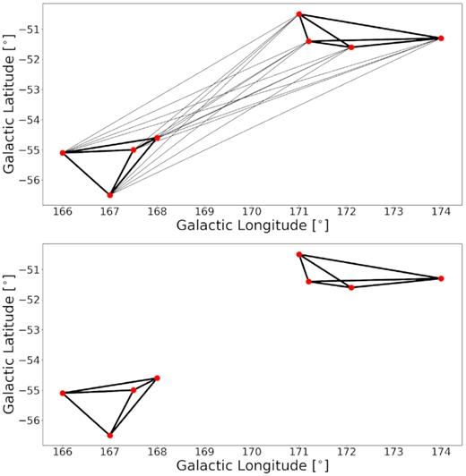
Graph representation of a single group after averaging over many runs. Points represent galaxies in the 2MRS survey. Edges are weighted according how often the connected pair were found in the same group. Thick edges represent pairs where galaxies were found |${\gt}90 {{\ \rm per\ cent}}$| of the time, thin edges pairs which were identified |${\lt}10{{\ \rm per\ cent}}$|. The top panel shows the group before weak edges are removed. The bottom panel shows how the group is split into two groups after the weak edges were removed.
This visualization technique provides a synergistic medium between human and computer understanding. A simple inspection of the points in Fig. 2 (in this particular example) clearly demonstrates that these two groups really are separate entities when overlaid with weighted edges. Averaging over many runs using graph theory and only considering statistically significant groupings and physical linking lengths (by removing weak edges) results in a stable and robust algorithm. In other words, the same group catalogue is generated regardless of the initial starting point of the algorithm or the order in which the algorithm cycles through the galaxies – an outcome which is not guaranteed in the traditional FoF algorithm.
We define two metrics with respect to the graph itself, namely the total and average connectedness score. These two global group statistics quantify the reliability of a group given the strength of its edges and the number of members. Indeed, the total connectedness score can be thought of as the corresponding number of nodes which make a complete graph (a graph where each node is connected to every other node) while the average connectedness score would represent the number of members of a group found in every single run. For example: a group might have 20 group members, with a total connectedness score of only 10. This would imply that it could be a group of 10 members found in every single run, with an additional 10 members found at a lower weighting or connectedness, while still satisfying the criterion of at least 50 |${{\ \rm per\ cent}}$| repeatability.
These are the metrics that we later use to identify groups that seem unstable and require further inspection by visual examination.
2.3 Identifying substructure
The graph description of each individual group furthermore allows for an innovative method of identifying substructure within groups, therefore extending the capabilities of the original FoF algorithm.
Cutting at a fixed significance level ensures robustness. However, cutting at higher significance levels can, in some cases, result in a group being sub-divided further. In order to combat the pseudo-randomness of the significance cut, we inspected every group to determine whether a stricter significance cut would result in separating groups. If this is the case, we identify these as substructures in a given group.
For every group, edges are iteratively removed from the graph from lowest to highest weighting, and with every iterative cut the number of subgraphs with three or more nodes is calculated. Once all edges have been removed, the maximum number of subgraphs with the lowest edge-cut become the subgroups.
Fig. 3 shows an example of such a case. The entire system is identified as a single group because all edges in Fig. 3 are within the cut-off limit of 50 per cent. However, if the cut-off limit had been set to 70 per cent, then the weak edges would have been removed, resulting in two independent groups (in the same way as the groups in Fig. 2). Removing edges sequentially from weakest to strongest results in two separate structures being identified. These substructures are classified as subgroups. In Fig. 3, the subgroups are represented by the two large red circles.
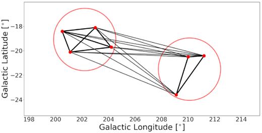
Graph representation of a group with sub-groups. Nodes represent galaxies in the 2MRS. Edges are weighted according to the percentage of the runs in which a galaxy pair is found for the same group. Strong edges represent |${\gt}90 {{\ \rm per\ cent}}$|, weak edges between |$60 \!-\! 70 {{\ \rm per\ cent}}$|. The two circles show the two subgroups identified when using our method.
2.4 Correcting for unreliable connections
A lot of effort has been put into addressing shortcomings of the FoF algorithm, since it is so easy to connect non-physical groups because of chance alignments. The graph method provides a powerful tool to correct for this. Nevertheless, a remnant of this issue remains for more complicated systems (such as the Virgo Supercluster); it is still possible for two or more obviously disconnected groups to be assigned to a single group and in some cases a low number of edges/connections can remain after a significance cut.
In some cases, visual evidence seems to suggest that two groups may be distinct and are arbitrarily connected through a single connection. However, computationally the entire system is seen as a single group and it is non-trivial to separate it into two distinct entities. This problem is compounded by the fact that there might be more than one unreliable connection. Determining what is an acceptable level of connections between these two groups before they are thought of as a single group is a challenging exercise. Furthermore, removing single edges and looking for a split in the group quickly becomes computationally exhaustive and is near impossible for cases where there is more than one connection.
In order to solve this issue, we looked at the average connectedness score of every group and whether or not those groups had any subgroups. The average connectedness of groups becomes a useful metric to flag these cases: when two obviously-separated group have very few connections, the number of connections in the group are less than the total number of possible connections. Thus, the average connectedness score is very sensitive to such situations and looking for groups with low values of this statistic that have subgroups immediately allows us to flag this issue.
While this artefact exists for less than 1|${{\ \rm per\ cent}}$| of the total groups, it is still important to correct for it. The best solution is to simply allow the subgroups to become their own groups. Any galaxies not identified as belonging to a subgroup were assigned to the nearest on-sky subgroup, as long as the value of R200 (defined in equation 13) of that subgroup was greater than the distance to the leftover galaxy.
Fig. 4 shows the 3D representation of the Virgo Supercluster as found in the 2MRS. There are two visually evident structures, which were identified as a single group before applying the correction described in Section 2.4. The edges shown in Fig. 4 are all |${\gt}70{{\ \rm per\ cent}}$| and both structures are connected to one another because of a single connection occurring at the |${\gt}70{{\ \rm per\ cent}}$| level. Thus, applying increasingly stricter cuts does not split the independent structures. This is the problem that the correction described in Section 2.4 aims to address. After this correction all three structures are identified as their own independent groups. Besides the main Virgo cluster, the now independent groups were identified as Virgo II groups (in particular the M61 and NGC 4753 groups at l = 298.99° and b = 66.3° and the NGC 4697 and NGC 4699 groups at l = 306.11° and b = 53.7°) and form part of the Virgo southern extension (Nolthenius 1993; Giuricin et al. 2000; Karachentsev & Nasonova 2013; Kim et al. 2016).
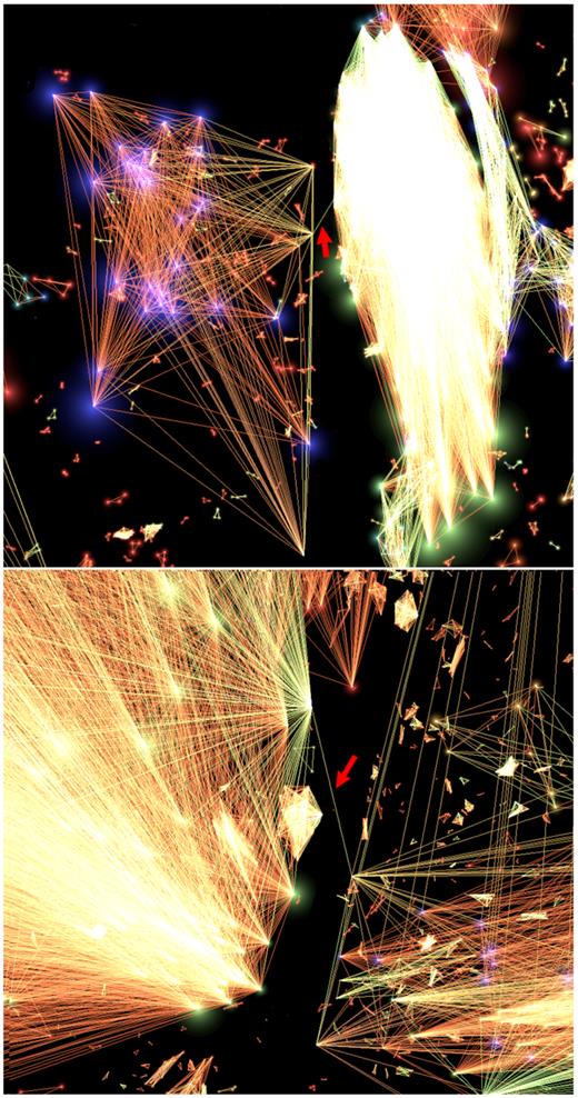
3D visualization of the Virgo Supercluster. The two large (independent structures) are both identified as a single group before corrections (as described in Section 2.4) are made. Green, orange, and red points represent galaxies with a scores of |${\gt}70{{\ \rm per\ cent}}$|, |${\gt}80{{\ \rm per\ cent}}$|, and |${\gt}90{{\ \rm per\ cent}}$|, respectively. The top and bottom panels show a normal and zoomed-in view of the false connection, respectively.
2.5 Linking lengths
Ramella et al. (1989) measured the number of groups, total number of galaxies in groups, the median velocity dispersion, and the first and third quartiles of the median velocity dispersion for the 6○ and 12○ CfA (Huchra & Geller 1982) survey as well as a mock catalogue of the survey by de Lapparent, Geller & Huchra (1986). This was done for varying linking lengths, with D0 = 0.56 Mpc and v0 = 350 km s−1 found to be the optimum choice of linking lengths at limiting the number of interlopers but not breaking apart large clusters. These same optimum linking lengths were later verified again in Ramella et al. (1997) for the Northern CfA2 survey (Huchra, Geller & Corwin 1995). They measured numerous group properties for several different linking lengths, which were compared to a geometric simulation of the sample. The linking lengths were also validated in Ramella et al. (2002) on both the Updated Zwicky Catalog and Southern Sky Redshift Survey (Falco et al. 1999; Ochsenbein, Bauer & Marcout 2000). Later, this combination of linking lengths was applied successfully to earlier versions of the 2MRS (namely Crook et al. 2007). In summary, this linking length choice of D0 = 0.56 Mpc and v0 = 350 km s−1 has been successfully used over four different surveys (including an earlier 2MRS survey) and has been validated by several independent methods.
The parameter choice is discussed further in the next section by evaluating it against our own mock catalogue. In order to incorporate the graph structure, we vary D0 and v0 between 0.56 ± 0.1 Mpc and 350 ± 100 km s−1, respectively, over 100 runs using 2 kpc and 2 km s−1 steps, respectively). The larger linking lengths will accommodate large clusters with dispersions of 1000 km s−1 given their larger gravitational potential wells.
Our choice of linking length parameter was validated against a 2MRS-like mock catalogue, generated by the Theoretical Astrophysical Observatory (TAO; Bernyk et al. 2016) described in the next section. The mock is complete up to |$K_{\rm s}^{\rm o} = 14{_{.}^{\rm m}}75$|, i.e. three magnitudes deeper than the 2MRS and contains both cosmological and peculiar redshifts.
2.6 Validation of algorithm on a mock catalogue
The TAO mock catalogue was used to (1) evaluate the choice of linking lengths set by Ramella et al. (1997) and (2) substantiate how accurately groups are recovered in the 2MRS given the relatively modest magnitude limit of |$K_{\rm s}^{\rm o}\lt 11{_{.}^{\rm m}}75$| and the effect of incompleteness as a function of magnitude limit and observed recession velocity.
2.6.1 Validating parameter choice
All three metrics were used in order to justify our choice of central linking lengths, which coincide with the studies of Ramella et al. (1997) and Crook et al. (2007). The results of running different parameters, which are then compared to the groups in the cosmological mock, are shown in Fig. 5. The top-left and top-right panels show reliability and completeness, respectively. When linking lengths are strict the reliability score is large, whereas large linking lengths have the opposite effect. The inverse is true for the completeness metric: when linking lengths are small, fewer groups make the cut (reducing completeness); however, the groups that do make the cut are recovered in the mock. Alternatively, when linking lengths are large, many groups pass the cut; however, the probability of false detections increases and a drop in reliability is seen. The completeness and the reliability results both provide a useful sanity check. Reliability tends to be lower than completeness in general. When visually inspecting the mock catalogue, the effect of redshift distortions is evident. Chance alignment of galaxies, in combination with a large spread in velocity due to peculiar motions in groups and large-scale cosmic flows, cause several false detections. This effect cannot be removed and is a consequence of identifying groups in redshift space. It is important to keep this in mind when using this (or any other) redshift-based group catalogue.
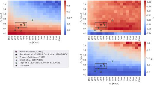
Completeness (top left), reliability (top right), and VI (bottom right) results when comparing groups found in the purely cosmological TAO mock catalogue to groups found by running our group finder on the redshift-distorted TAO mock over several different parameter choices. Each pixel represents a comparison. The v0 and D0 parameters for each individual run form the x and y axes, respectively. Stars represent the parameters chosen by previous works. The black square shows the range of parameters probed by this work when implementing the graph theory method discussed in Section 2.2.
The VI results show where we could optimize both completeness and reliability. We overlay the parameter choices used by several different authors also running FoF algorithms. Of particular interest is the black star, which represents the parameter choice used by Ramella et al. (1997) and later Crook et al. (2007) that we adopt in this work. The range of parameters spanned by our group finder (making use of the graph theory adaptation discussed in Section 2.2) is demarcated in Fig. 5 as a black rectangle.
The Ramella et al. (1997) parameters result in a reliability R > 0.7 and a completeness of C > 0.8. These parameters also have low VI scores, implying a reasonably good recovery of the mock groups. The Ramella et al. (1997) linking lengths are also close to values used by other authors. All linking lengths chosen by previous authors seem to hover around the VI ‘well’ in Fig. 5.
2.6.2 Evaluating incompleteness
The mock was used to substantiate how accurately groups are recovered in the 2MRS given the relatively modest magnitude limit of |$K_{\rm s}^{\rm o}\lt 11{_{.}^{\rm m}}75$| and the effect of incompleteness as a function of magnitude limit and observed recession velocity. The group finder was run on the TAO mock with a magnitude limit of |$K_{\rm s}^{\rm o}\lt 11{_{.}^{\rm m}}75$|. Groups with three members (representing the extreme case of low number statistics) were identified, providing the base for all future comparisons. The group finder was then run on increasingly deeper subsets of the mock in steps of |$\Delta m = 0{_{.}^{\rm m}}25$| up to |$K_{\rm s}^{\rm o}\lt 14{_{.}^{\rm m}}75$| (see x-axis of Fig. 6).
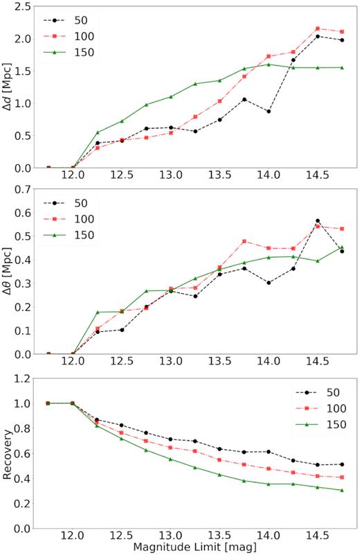
Trends of galaxy groups with three members found in the TAO mock catalogue at the 2MRS magnitude limit of |$K_{\rm s}^{\rm o}\lt 11 {_{.}^{\rm m}}75$|, as a function of magnitude completeness limit (x-axis) and distance (different curves). The solid, dashed, and dotted lines represent groups with a co-moving distance of 0 < d ≤ 50 Mpc, 50 Mpc < d ≤ 100 Mpc, and 100 Mpc < d < 150 Mpc, respectively. Top: offset in line-of-sight position with changing depth. Middle: projected on-sky offset with changing depth. Bottom: percentage of the total group recovered at a magnitude limit of |$K\lt 11 {_{.}^{\rm m}}75$|. This plot quantifies how accurately positions of groups are recovered and what percentage of the group members are found.
The groups with three members found at |$K_{\rm s}^{\rm o}\lt 11 {_{.}^{\rm m}}75$| were re-identified in subsequent, deeper runs of the group finder on the mock. Their positions (both on sky and line of sight), the total number of members at each magnitude cut, and the difference of various group parameters compared to the |$K_{\rm s}^{\rm o}\lt 11 {_{.}^{\rm m}}75$| limit were noted. These groups were then grouped into three distance bins of 50, 100, and 150 Mpc. Finally, the difference in the three-member group properties of the actual 2MRS were compared to the stepwise increased magnitude limit in the mock for each bin and are presented in the three panels of Fig 6.
The top panel in Fig. 6 shows how the line-of-sight position of the group changes with deeper magnitude cuts. We note that line-of-sight positional offsets, i.e. the radial velocity axis, tend to increase with depth and slowly level off around 2 Mpc. This relatively large offset in line-of-sight position can be attributed to the well-known ‘finger-of-god’ effect. It never exceeds an Abell radius, though.
The middle panel shows the projected on-sky offset with depth. The average offset is less than 0.5 Mpc. This is much less than the error in the radial direction because there is no velocity distortion on the plane of the sky, other than the diminutive Kaiser flattening effect. Both the line-of-sight and on-sky offsets appear to be independent of the distance of the groups.
The bottom panel shows the percentage of the group present in a survey limited at |$K_{\rm s}^{\rm o} \le 11 {_{.}^{\rm m}}75$|. Unsurprisingly, there is a very clear trend with distance. Nearby groups are less affected by incompleteness than those at large distances. Thus, the fraction of recovered members is greater for nearby groups. We provide a correction to the group membership number based on the luminosity function of the relatively complete Virgo Supercluster, see Section 4.2.4.
It is important to keep these offsets and incompleteness in mind when making use of this group catalogue.
3 VISUALIZATION TECHNIQUES
We made use of the state-of-the-art visualization laboratory hosted by the Institute of Data Intensive Astronomy (IDIA), which includes immersive displays and notably a virtual reality (VR) system that is ideal for 3D data sets. We were able to efficiently compare our group results (based on running the algorithm with our choice of linking length) against the intrinsic large-scale structure distribution provided by the mock. Fig. 7 shows how well the algorithm recovers real groups using our choice of linking length parameter, by overlaying the groups that were found over the positions of the galaxies in the TAO mock.

Example of a group identified in the TOA mock. The pink sphere shows the location of the group as found in the distorted mock (right), and is overlaid in the undistorted mock (left). This shows that the FoF algorithm finds physical groups whilst being run on a redshift distorted data set. A 3D video of this plot can be found here.
3.1 Visualization facilities
As mentioned, the catalogue was tested and verified using the new state-of-the-art visualization facilities hosted by IDIA. This included the use of VR, a panorama immersive facility, and the 8K digital planetarium dome housed at the Cape Town Iziko Museum. Using these facilities provides an additional supplement to the standard methods of bug-finding. This is achieved by overlaying several data sets, plus a variety of visual markers. This can consist of several other markers that can be used as diagnostic tools such as spheres (designating radius), lines connecting associated galaxies of the same group, colour palettes characterizing distance.
Every run of the algorithm and technical change made to the group finder was interrogated against previous renditions using the visualization lab, to inspect the results and ensure that (1) no logical errors were present in the updated version, and (2) that changes rendered better results than previous iterations.
3.2 Rebuilding the traditional fof algorithm
We first built a group-finder using the same method described in Crook et al. (2007) and applied it to the early (shallower and incomplete) version of 2MRS. The two group catalogues were then compared using VR in addition to running our new algorithm on this same data set. The galaxies from Crook et al. (2007) were portrayed as small points in three dimensions using Cartesian Galactic coordinates. Both group catalogues were displayed as large blue and red spheres (for Crook et al. 2007, and our results, respectively). The spheres mix colours in the virtual environment creating an overlap of purple (in this particular case). In this way it is possible to see at a glance (a) an agreement of the two catalogues (purple spheres) and (b) numerous types of discrepancies including line-of-sight offsets, on-sky offsets, groups found by our catalogue but not by Crook et al. (2007), and vice versa.
3.3 Visualizing graphs
Using graph theory to average over the runs allowed us to think of each group as a topological data set, and as such they optimally lend themselves to visualization (Pascucci et al. 2011). This was accomplished by looking at pairs of galaxies, and deriving the frequency with which pairs were put in the same group. This results in a completely novel way of constructing a group catalogue, and solving the degeneracy issue arising from averaging over a three-dimensional data set.
Furthermore, we developed a unique approach in visualizing the multiple results by translating the mathematical graph objects from graph space into redshift space. Visual examination of the dataset then provides instantaneous feedback of both the underlying group finder and simultaneously the underlying mechanisms that led to those results.
Fig. 8 shows an example of how the results of our group finder were visualized for any given group. Having the graphs displayed in this fashion allowed for exploration on how the graph structures themselves could be better used to improve the group results. This optimization was done by making use of (1) the mock catalogue, which has both redshift and distance information; (2) well-known clusters and groups in the full 2MRS catalogue; and (3) any examples of groups which were found to be suspicious. The latter option was of particular importance, and possible only thanks to the powerful 3D visualization techniques. Finding examples of failures of the algorithm (e.g. where two obviously separate groups were connected as one) is straightforward when using visual inspection in VR and allows for exploration of intrinsic weaknesses of the group finder algorithm.

Three-dimensional example of a group with the resulting graph overlaid. Points represent the positions of 2MRS galaxies. Edges represent the number of connections of galaxies in the same group. Red edges represent 90–100 |${{\ \rm per\ cent}}$| and blue edges represent 0–|$10{{\ \rm per\ cent}}$|. A video displaying these connections in 3D is available here.
3.4 Removing statistical outliers
Visual inspection reveals that averaging over all results is not good enough. While the robustness of the method is assured, groups can become too large because of a single connection/edge between two obviously distinct groups (see e.g. Fig 4). It also is unrealistic to accept every single connection. A galaxy which is associated with a group for |$10{{\ \rm per\ cent}}$| of the runs but with another one for the remaining |$90{{\ \rm per\ cent}}$| is much more likely to form part of the latter. In other words, while the robustness of the method is assured, robustness to statistical outliers is not and a significance cut must be made. A careful analysis based on both the mock catalogue and well-known groups and clusters indicated that accepting connections at the |${\gt}50{{\ \rm per\ cent}}$| level occurrence gives the best results. Using the graph tool was highly effective here; a removal of all edges with a weighting |${\lt}50{{\ \rm per\ cent}}$| was sufficient to disconnect subgraphs. At this point, the group finder is stable. An example of this process is shown in Fig. 8. Edges are coloured according to the percentage of runs in which a galaxy pair was assigned to the same group. Frames (A) and (B) display the galaxy group on the plane of the sky while (C) and (D) show the distribution along the line of sight. Frames (A) and (C) show the group before the cut was implemented, while frames (B) and (D) show the effect of the cut. Note that if the cut had not been implemented (i.e. removal of low-weighted, blue edges) then the entire system would have been classified as a single group. However, confusion can sometimes occur in situations where groups are radially aligned coincidentally.
3.5 Subgroups
On the other hand, we also came across several groups that seemed to have two or more concentrations of galaxies. If the statistical cut had been stricter than |$50{{\ \rm per\ cent}}$| (say |$60{{\ \rm per\ cent}}$| or |$70{{\ \rm per\ cent}}$|) then they would have split into separate groups. To account for these cases, a higher statistical cut was applied to each group to check the likelihood of them having real substructure, and/or whether some of these subgroups are real. Differentiation of these cases was easy in VR; however, translating this visual information into an algorithmic equivalent is quite a challenge. The connectedness score described in equation (6) achieved this goal – colouring the galaxies by this property made the groups that required attention stand out clearly. Based on this information, we could identify groups with low average connectedness score and which also contained subgroups. In these cases, these subgroups became their own groups.
Fig. 9 gives an illustration of a group with subgroups. From frame (A) to (C), lines of decreasing strengths are removed until no more lines can be cut. The number of separate structures changes from one in frame (A) to two in frames (B) and (C). Because the maximum number of isolated systems is two, subgroups are chosen to be the first instance at which the maximum number of isolated systems occurs [frame (B) in this particular example].
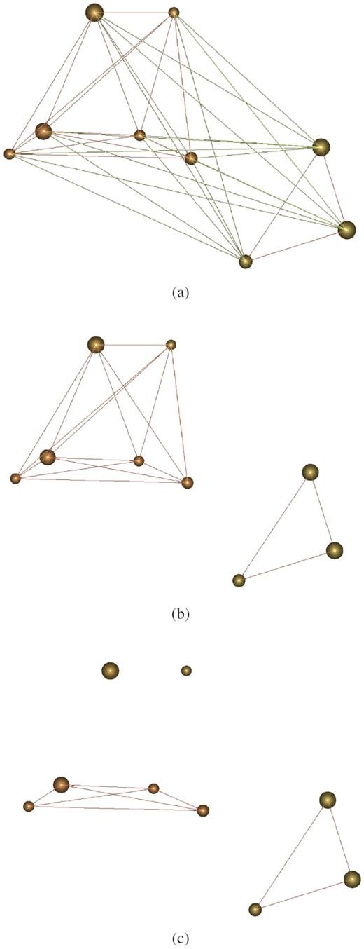
Example of a galaxy group containing two subgroups and highlighting the method of identifying subgroups by incrementally removing the weakest edges. Panel (A) shows the group with all edges |${\ge}50{{\ \rm per\ cent}}$| still present, panel (B) shows the group after edges with a weighting of |$60{{\ \rm per\ cent}}$| and less are removed, and panel (C) shows the group when edges with a weighting of |$80{{\ \rm per\ cent}}$| and less are removed, resulting in only the strongest edges remaining (in this case edges with a weighting of 1). A 3D-animation of these examples is available here.
The use of numerous visualization techniques enabled us to identify issues affecting the traditional FoF algorithm and make various updates to address them. These included (1) running the algorithm many times; (2) averaging over all runs using graph-theory; (3) removing statistical outliers by implementing a significance cut; (4) applying a recursive cut to graphs to find any subgroups; and (5) identifying weak and non-physical connections and correcting these groups.
4 THE 2MRS GROUP CATALOGUE
Our final 2MRS group catalogue contains 3022 entries and is the most complete ‘whole-sky’ galaxy group catalogue to date. We provide measured and calculated group properties, such as: 3D positions, luminosity, and comoving distances, observed and corrected number of members, richness metric, velocity dispersion, and estimates of R200 and M200.
4.1 Measured group properties
The measured group properties include the velocity dispersion and the projected central position, which in turn affect many of the other derived quantities. Thus, we elaborate on these below.
4.1.1 Velocity dispersion
4.1.2 Projected group centre
There have been several proposed methods of determining the projected group centre amongst different surveys and catalogues (Crook et al. 2007; Poggianti et al. 2010; Robotham et al. 2011; Tempel et al. 2018). Several techniques were explored using the TAO mock catalogue, such as luminosity-weighted and flux-weighted moments, and the simple geometric centre. We found that taking the average RA and Dec. of the group members rendered the most accurate central on-sky position, both when inspecting the mock catalogue and identifying well-known existing groups and clusters.
4.1.3 Projected radius
The projected radius was calculated as the maximum projected on-sky distance of all the galaxies from the projected group centre. While this method is not robust against outliers, we found that those could be robustly identified and corrected using the new visualization techniques.
The projected radius was calculated as the maximum projected on-sky distance of all the galaxies from the projected group centre. While this method is not robust against outliers, it was found that those could be robustly identified and corrected using the new visualization techniques as visual spheres with radii equal to the projected radius metric would become hugely exaggerated, immediately highlighting problematic groups and methods which were then ultimately corrected, resulting in the complete catalogue having no such issues.
4.2 Calculated group properties
4.2.1 R200 and M200
4.2.2 Comoving and luminosity distances
4.2.3 Richness
A simple definition of richness similar to Andreon (2016) is included in the catalogue. We define richness as the number of galaxies within a group with absolute magnitude of |$M_K^{\rm o}\lt -23{_{.}^{\rm m}}5$|. This definition is maintained up to 100 Mpc where the survey is still reasonably complete. The richness is still calculated for groups greater than 100 Mpc but this value would represent the minimum richness possible and is reported as such in the final catalogue.
4.2.4 Corrected group members
4.3 Catalogues
We present one main and two supplementary 2MRS group catalogues, as detailed below.
4.3.1 The 2MRS catalogue
The main 2MRS group catalogue is presented in Table 1. The 20 groups with the highest membership are shown for explanatory purposes, while the full table is available online. The columns are
2MRS group ID as defined in this work.
Names (where available) of well-known groups and clusters in other catalogues.
Average RA (α) of the group, in degrees.
Average Dec. (δ) of group, in degrees.
Average Galactic longitude (l) of the group, in degrees.
Average Galactic latitude (b) of the group, in degrees.
Number of 2MRS galaxies in the group.
Corrected number of members, calculated using equation (16).
Richness, as defined in Section 4.2.3.
Recession velocity, in the CMB reference frame.
Co-moving distance, calculated using equation (15).
Luminosity distance, as defined in Section 4.2.2.
Velocity dispersion, calculated using equation (12)
Velocity dispersion given by the standard deviation of the velocities of members of the group.
R200 value, calculated using equation (13).
M200 value, calculated using equation (14).
Number of subgroups, as defined in Section 2.3.
2MRS galaxy group catalogue.
| Group ID | Other names | α | δ | l | b | Nmem | |$N^{\prime }_{\text{mem}}$| | R | vcmb | dc | dL | RMS | σ | R200 | M200 | Nsubs |
|---|---|---|---|---|---|---|---|---|---|---|---|---|---|---|---|---|
| (deg, J2000) | (km s−1) | (Mpc) | (km s−1) | (Mpc) | (×1011 M⊙) | |||||||||||
| (1) | (2) | (3) | (4) | (5) | (6) | (7) | (8) | (9) | (10) | (11) | (12) | (13) | (14) | (15) | (16) | (17) |
| 2987 | VIRGO CLUSTER | 187.80 | 11.41 | 285.13 | 73.58 | 163 | 163 | 36 | 1523 | 20.8 | 20.9 | 486 | 484 | 1.15 | 188.5 | 0 |
| 153 | ABELL 3627 | 243.67 | −60.89 | 325.27 | −7.17 | 121 | 278 | 67 | 4931 | 67.3 | 68.4 | 854 | 861 | 2.01 | 1015.6 | 3 |
| 50 | ABELL 3526B | 192.03 | −41.21 | 302.26 | 21.66 | 102 | 177 | 45 | 3784 | 51.7 | 52.3 | 795 | 792 | 1.87 | 820.8 | 3 |
| 3031 | ABELL 0426 | 49.76 | 41.38 | 150.53 | −13.45 | 95 | 224 | 47 | 5158 | 70.4 | 71.6 | 702 | 714 | 1.65 | 564.4 | 0 |
| 228 | COMA CLUSTER | 194.90 | 28.00 | 59.10 | 87.99 | 95 | 360 | 78 | 7260 | 98.9 | 101.3 | 734 | 751 | 1.72 | 643.8 | 3 |
| 179 | – | 159.12 | −27.66 | 269.64 | 26.35 | 85 | 156 | 25 | 4043 | 55.2 | 56.0 | 604 | 611 | 1.42 | 360.2 | 0 |
| 271 | ABELL 0262 | 28.44 | 36.23 | 136.75 | −24.96 | 61 | 129 | 25 | 4630 | 63.2 | 64.2 | 450 | 457 | 1.06 | 148.7 | 0 |
| 3011 | – | 181.50 | 46.19 | 145.21 | 68.92 | 61 | 61 | 4 | 993 | 13.6 | 13.6 | 193 | 193 | 0.46 | 11.9 | 0 |
| 500 | ABELL 1367 | 176.15 | 19.97 | 234.45 | 73.12 | 56 | 194 | 44 | 6787 | 92.5 | 94.6 | 610 | 623 | 1.43 | 368.4 | 0 |
| 151 | ABELL S0805 | 281.49 | −63.03 | 332.53 | −23.38 | 56 | 111 | 31 | 4392 | 60.0 | 60.8 | 429 | 424 | 1.01 | 129.2 | 0 |
| 25 | ERIDANUS CLUSTER | 54.21 | −20.12 | 211.53 | −51.64 | 53 | 53 | 5 | 1517 | 20.8 | 20.9 | 251 | 250 | 0.59 | 26.1 | 0 |
| 84 | HYDRA CLUSTER | 157.79 | −35.36 | 273.17 | 19.27 | 51 | 76 | 17 | 3155 | 43.1 | 43.6 | 513 | 517 | 1.21 | 221.0 | 2 |
| 4 | FORNAX CLUSTER | 53.93 | −35.02 | 236.00 | −54.21 | 49 | 49 | 9 | 1357 | 18.6 | 18.7 | 296 | 295 | 0.70 | 42.3 | 0 |
| 202 | – | 17.31 | 32.65 | 127.26 | −30.08 | 48 | 107 | 21 | 4838 | 66.0 | 67.1 | 412 | 417 | 0.97 | 114.3 | 2 |
| 150 | – | 193.67 | −13.77 | 304.14 | 49.10 | 48 | 106 | 20 | 4718 | 64.4 | 65.4 | 323 | 328 | 0.76 | 54.8 | 3 |
| 369 | OPH CLUSTER | 258.06 | −23.39 | 0.53 | 9.30 | 46 | 250 | ≥46 | 8757 | 119.2 | 122.6 | 792 | 812 | 1.85 | 804.5 | 2 |
| 101 | – | 20.83 | 33.54 | 130.51 | −28.86 | 46 | 97 | 20 | 4614 | 63.0 | 64.0 | 453 | 460 | 1.07 | 151.8 | 0 |
| 261 | – | 193.35 | −9.26 | 303.75 | 53.61 | 45 | 92 | 16 | 4473 | 61.1 | 62.0 | 365 | 369 | 0.86 | 79.4 | 2 |
| 355 | – | 107.01 | 49.74 | 167.35 | 22.93 | 44 | 128 | 27 | 6032 | 82.2 | 83.9 | 281 | 286 | 0.66 | 36.1 | 3 |
| 142 | – | 206.98 | −30.39 | 317.13 | 30.92 | 44 | 98 | 21 | 4853 | 66.2 | 67.3 | 419 | 424 | 0.99 | 120.2 | 0 |
We have plotted both richness (column 9 in Table 1) and the number of corrected members, |$N^{^{\prime }}_{\rm mem}$| (column 7 in Table 1) against R200 in Figs 10 and 11, respectively. R200 is determined solely by the dispersion of the group, unlike richness and Nmem that are entirely independent of dispersion. It therefore is necessary to have both the number of members and richness increase with R200. Our definition of richness also shows a tight relation with R200 which is a good validation of our procedure. The extreme outlier present in Fig. 11 is the Virgo Supercluster. Figs 10 and 11 show the integrity of the main catalogue.
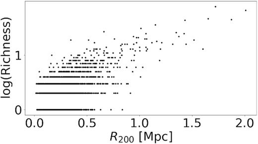
Relation between group richness (Section 4.2.3) and R200.
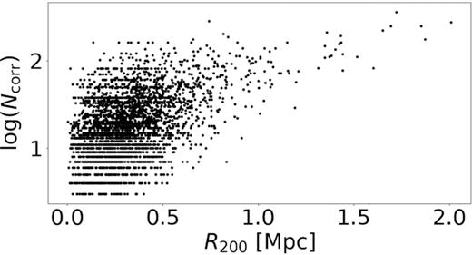
Relation between number of corrected group members and R200.
4.3.2 The 2MRS subgroup catalogue
A subgroup catalogue is also included, with a random sub-sample shown in Table 2. The subgroup catalogue includes Group ID, mean values of α, δ, l, and b, vcmb, and Nmem as described in Table 1. The sub ID, (1) in Table 2, demarcates the unique identifier for each individual subgroup. The ID is made up of two parts, namely the host galaxy group ID (the group to which said subgroup belongs) and the numbered subgroup within said host group.
2MRS subgroup catalogue.
| Sub ID | Group ID | α | δ | l | b | vcmb | Nmem |
|---|---|---|---|---|---|---|---|
| (deg, J2000) | (km s−1) | ||||||
| 1000-1 | 1000 | 140.72 | 24.44 | 203.96 | 43.31 | 10337 | 4 |
| 1000-2 | 1000 | 141.60 | 23.89 | 204.98 | 43.94 | 10145 | 3 |
| 1015-1 | 1015 | 107.14 | −49.10 | 259.72 | −17.53 | 12790 | 7 |
| 1015-2 | 1015 | 106.12 | −48.98 | 259.35 | −18.11 | 12997 | 3 |
| 1031-1 | 1031 | 241.04 | 69.77 | 103.49 | 39.28 | 7540 | 3 |
| 1031-2 | 1031 | 239.39 | 70.74 | 104.93 | 39.22 | 7486 | 6 |
| 1091-1 | 1091 | 52.65 | 41.59 | 152.24 | −12.05 | 5367 | 7 |
| 1091-2 | 1091 | 52.56 | 40.53 | 152.81 | −12.95 | 4772 | 5 |
| 1093-1 | 1093 | 241.24 | 17.57 | 31.31 | 44.52 | 10395 | 17 |
| 1093-2 | 1093 | 241.48 | 18.00 | 31.99 | 44.46 | 11589 | 11 |
| 1100-1 | 1100 | 251.94 | 58.81 | 88.16 | 38.82 | 5256 | 3 |
| 1100-2 | 1100 | 249.56 | 57.86 | 87.30 | 40.25 | 5349 | 6 |
| 1154-1 | 1154 | 52.59 | 41.79 | 152.08 | −11.92 | 4325 | 3 |
| 1154-2 | 1154 | 52.13 | 40.29 | 152.68 | −13.34 | 4107 | 3 |
| 1186-1 | 1186 | 195.68 | −56.21 | 304.51 | 6.63 | 6225 | 4 |
| 1186-2 | 1186 | 196.91 | −57.33 | 305.13 | 5.47 | 6030 | 13 |
| 119-1 | 119 | 142.76 | −61.89 | 281.56 | −7.66 | 2862 | 17 |
| 119-2 | 119 | 137.59 | −64.03 | 281.46 | −10.82 | 2076 | 4 |
| 1201-1 | 1201 | 173.22 | −9.62 | 272.85 | 48.61 | 6630 | 21 |
| 1201-2 | 1201 | 174.68 | −9.32 | 274.62 | 49.52 | 6155 | 4 |
4.3.3 The 2MRS galaxies in groups catalogue
We also include a catalogue consisting of all the galaxies that are member of a group in Table 3. This catalogue includes the 2MASS ID, α, δ, l, b of each galaxy as given in Macri et al. (2019), as well as our calculated vcmb, Group ID from Table 1 and Sub ID from Table 2. A random sub-sample of galaxies are shown in Table 3 for reference.
2MRS group member catalogue.
| 2MASS ID | α | δ | l | b | vcmb | Group ID | Sub ID |
|---|---|---|---|---|---|---|---|
| (deg, J2000) | (km s−1) | ||||||
| 02284905 + 3810005 | 37.20436 | 38.16689 | 143.22255 | −20.83781 | 11189 | 1541 | 1541-2 |
| 10032864−1530044 | 150.86940 | −15.50126 | 254.13606 | 31.03521 | 9998 | 1763 | – |
| 04375557−0931092 | 69.48154 | −9.51926 | 205.99341 | −33.93850 | 5110 | 724 | – |
| 02362379+3142410 | 39.09909 | 31.71140 | 147.68501 | −26.06654 | 4705 | 152 | 152-2 |
| 16175726−6055229 | 244.48875 | −60.92303 | 325.53091 | −7.47124 | 3597 | 153 | 153-3 |
| 08333766+5535322 | 128.40689 | 55.59229 | 162.22017 | 36.37661 | 11300 | 1971 | – |
| 01293373+1717532 | 22.39054 | 17.29812 | 135.76518 | −44.62148 | 12761 | 2535 | – |
| 14165292+1048264 | 214.22060 | 10.80737 | 357.96130 | 64.11185 | 7650 | 334 | – |
| 10081231 + 0958374 | 152.05138 | 9.97701 | 229.02748 | 47.94034 | 8532 | 2188 | – |
| 02442183+3121169 | 41.09096 | 31.35475 | 149.54651 | −25.61624 | 5203 | 152 | 152-1 |
| 14034273−3243006 | 210.92809 | −32.71685 | 320.07907 | 27.73697 | 4028 | 85 | – |
| 09202342+5456313 | 140.09766 | 54.94210 | 161.67014 | 43.04770 | 13827 | 2358 | – |
| 17281491−6640152 | 262.06204 | −66.67094 | 325.71674 | −17.07140 | 13589 | 193 | – |
| 23000358+1558493 | 345.01495 | 15.98034 | 87.56570 | −39.12365 | 1828 | 354 | – |
| 13295512−3119561 | 202.47968 | −31.33226 | 312.50024 | 30.82352 | 15142 | 1782 | – |
| 21073236−2538350 | 316.88477 | −25.64310 | 21.20206 | −40.26195 | 11998 | 818 | – |
| 12492664−4127463 | 192.36107 | −41.46286 | 302.53073 | 21.40733 | 5086 | 50 | 50-1 |
| 13331326+3306350 | 203.30525 | 33.10971 | 68.98088 | 79.17372 | 7636 | 149 | – |
| 17030344+6102381 | 255.76439 | 61.04391 | 90.49467 | 36.52942 | 3391 | 839 | – |
| 19324667−6431251 | 293.19467 | −64.52367 | 331.77798 | −28.70660 | 4233 | 806 | – |
| 02094273−1011016 | 32.42808 | −10.18383 | 174.08235 | −64.95735 | 3623 | 413 | – |
| 05393634+1259047 | 84.90136 | 12.98459 | 192.95486 | −9.49321 | 7229 | 2956 | – |
| 13170188−1046121 | 199.25781 | −10.76999 | 313.08246 | 51.59659 | 3153 | 1447 | – |
| 18492430−4846088 | 282.35126 | −48.76904 | 347.37582 | −19.73818 | 5244 | 2405 | – |
| 22120645+3720024 | 333.02695 | 37.33405 | 91.02950 | −15.47828 | 5632 | 189 | 189-2 |
| 03053667+0459396 | 46.40281 | 4.99440 | 173.28879 | −44.36787 | 8407 | 452 | – |
| 10512393+2806429 | 162.84979 | 28.11196 | 203.77824 | 63.45928 | 1562 | 124 | – |
| 06254878−5359361 | 96.45339 | −53.99345 | 262.68002 | −25.29278 | 14006 | 2636 | – |
| 09045016+1333424 | 136.20901 | 13.56185 | 215.39915 | 35.63015 | 8778 | 1879 | – |
| 02303366+3210342 | 37.64031 | 32.17624 | 146.21729 | −26.17465 | 4552 | 593 | – |
The on-sky distribution of the final 2MRS group catalogue is shown in Fig. 12. We have recovered all the well-known, large-scale structures and, in particular, the intricate substructures that comprise them. This bodes well in validating our group finding algorithm as the structures we recovered are similar to previous 2MRS-based catalogues (Crook et al. 2007; Saulder et al. 2016; Tempel et al. 2016; Kourkchi & Tully 2017; Tempel et al. 2018).
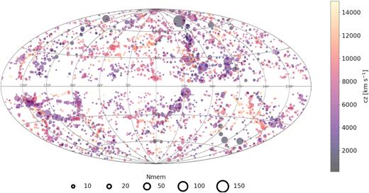
Aitoff projection in Galactic coordinates of the completed 2MRS group catalogue. Each symbol represents a group, with its size determined by the number of members and its colour related to the recession velocity. Only groups out to cz = 15 000 km s−1 are shown.
4.4 Comparisons to literature
In validating our results, it is important to compare our work with previous catalogues based on earlier versions of 2MRS, and to compare our method with other techniques. For the former, we compared our catalogue against Crook et al. (2007), Tempel et al. (2016, 2018), and Lim et al. (2017). Our cross-matching search was done using tolerances of 1 and 5 Mpc for plane-of-sky and line-of-sight distances, respectively. We choose these values to be conservative and expect matches to be well within 1 Mpc in the spatial plane and 5 Mpc in the radial. The resulting matches and discrepancies were investigated using the IDIA visualization lab.
4.4.1 Crook et al. (2007)
Crook et al. (2007) based their group finder on the classic FoF algorithm as developed by Huchra & Geller (1982) without any modification. This group finder was applied to an earlier and shallower 2MRS catalogue with a limit of |$K_{\rm s}^{\rm o} \lt 11{_{.}^{\rm m}}25$|. Nevertheless, since we built upon their techniques for our analysis, a comparison is appropriate.
Crook et al. (2007) used two different choices of linking length, resulting in two catalogues (respectively referred to as high- and low density). We only compared our results against the high-density catalogue since it used the same linking lengths proposed by Ramella et al. (1997) and adopted by us. We did not consider any groups found in this previous work that were based on artificial galaxies, which they used to fill the ZoA.
We recovered all groups detected by Crook et al. (2007). There are several groups consisting only of galaxies with |$K_{\rm s}^{\rm o}\gt 11 {_{.}^{\rm m}}25$| which are present in our catalogue but naturally are not in Crook et al. (2007). Interestingly, several groups in Crook et al. (2007) were identified at the lower and upper velocity ranges of large clusters. In other cases, large clusters (such as Virgo and Coma) that were made up of numerous groups in Crook et al. (2007) only contained one single large cluster in our catalogue. This is an example of ‘shredding’ that happens with large groups and clusters. Our method is robust against shredding, and hence this is one of the common differences we see in comparing with other catalogues, in this case Crook et al. (2007).
4.4.2 Tempel et al. (2016, 2018)
Tempel et al. (2016) created a modified version of the FoF algorithm in which membership refinement was included, making use of: (1) multimodality analysis (in an attempt to identify substructure within groups) and (2) determining the virial radius of groups and identifying any outliers from the escape velocity of the members (in order to not unjustifiably add members to groups). These techniques have direct analogies within our own method to achieve many of the same goals.
Their modified version of the FoF was applied to the Huchra et al. (2012) version of 2MRS, as well as to other redshift surveys. They compared the resulting 2MRS group catalogue with the Tully (2015) 2MRS group catalogue between 3000 and 10 000 km s−1.
Tempel et al. (2016, 2018) allowed groups with just two members, instead of our stronger requirement of 3 or more. We applied our criterion to their results to enable a consistent comparison with our work.
The most significant difference between the Tempel et al. (2016, 2018) catalogues are the methods used to identify groups. Whilst Tempel et al. (2016) relied on a modified FoF algorithm, Tempel et al. (2018) made use of a Bayesian group finder based on the method discussed in Stoica (2010). Once again, their algorithm was applied to the Huchra et al. (2012) catalogue.
As was the case in Crook et al. (2007), both Tempel et al. (2016, 2018) had incidents in which large and well-known clusters were separated into numerous groups, whereas these are identified as a single cluster by our procedures. This further validates the success of our graph theory implementation. Groups found by Tempel et al. (2016) or Tempel et al. (2018) and not found by us generally contained very few members and were often marginally connected. We attribute these cases (in Tempel et al. 2016) to a larger set of linking lengths which allowed for more marginal detections. Despite this, we do recover more groups in total than either Tempel et al. (2016) or Tempel et al. (2018) as seen in the distributions in Fig. 13.
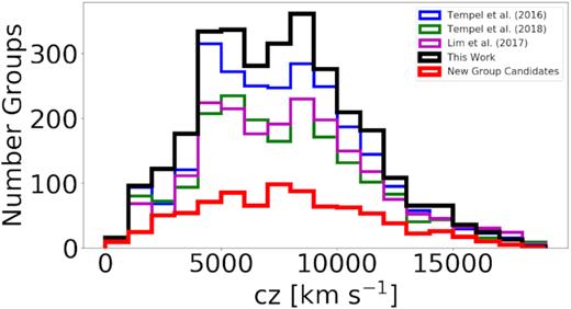
Number of groups as a function of redshift in our catalogue and previous analyses of 2MRS.
4.4.3 Lim et al. (2017)
Lim et al. (2017) has developed a halo-based group finder that was applied to four major redshift surveys, most notably the 2MRS. This halo-based finder provides a uniquely different method to both the FoF algorithm used by Crook et al. (2007) and Tempel et al. (2016) and the halo-based group finder of Tempel et al. (2018). This makes it a suitable candidate to compare to our own catalogue.
Lim et al. (2017) included groups with members ≥1. In order to make a fair comparison we only include groups with N ≥ 3.
This catalogue was the closest to our own. However, there was severe shredding present within many of the large, well-known clusters and we still recovered more groups than Lim et al. (2017).
Of particular interest is the case of Abell 3558 (Shapley), our method found multiple groups instead of one large cluster whereas (Lim et al. 2017) correctly identify the cluster. This was due to the incompleteness of 2MRS at these large distances.
4.4.4 New groups
New groups were identified as those with no match (within our tolerances) in the aforementioned catalogues. Fig. 13 shows their distribution as a function of redshift. Notably, their distribution is identical to the other catalogues, implying that new groups are being found around existing large-scale structures. This can be further verified from their spatial distribution, as seen in Fig. 14. For the most part it seems that the new galaxy group candidates are aligned with already well-known structures; however, there are several new ones that are found in underdense regions.
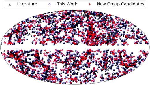
Galactic Aitoff projection showing the on-sky distribution of galaxy groups from Crook et al. (2007), Lim et al. (2017), and Tempel et al. (2016, 2018) as well as the groups found in this work. Black triangles show literature groups, blue circles show groups from this work, and red crosses demarcate possible new groups not found in literature.
Of particular interest is the ZoA, where the majority of the new redshifts in the final release of 2MRS were located. Fig. 15 shows a zoomed-in view of the ZoA (|b| < 25○). Once again, there are several new galaxy group candidates in regions of higher density as well as several along the ‘lip’ of the exclusion Zone. These particular groups will be interesting to follow up, as many align themselves with known structures deep within the ZoA (|b| < 10○, Staveley-Smith et al. 2016; Ramatsoku et al. 2016; Courtois et al. 2019).
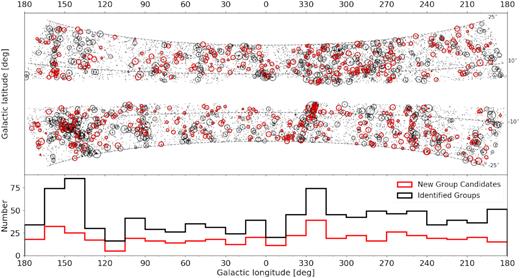
Zoomed-in view of the band around the ZoA (|b| < 25○). Top panel shows the on-sky distribution of galaxies and galaxy groups found in the ZoA. Circles represent groups found in this work. Black circles have a matching group in the literature. Red circles are groups without a match and are new group candidates. Bottom panel shows the distribution of the groups along the Galactic plane. Black line shows the distribution of all the groups in the 2MRS while the red shows the distribution of the new groups only.
As an additional exercise in examining the validity of our new galaxy group candidates, an extreme set of cross-matching criteria was chosen (6 and 12 Mpc in the plane of sky and along the line of sight, respectively) in order to identify the most likely new galaxy group candidates. Among these we selected 20 groups with five or more members, only five of which were previously identified in the NASA Extragalactic Database (NED); two are substructures of the well-known Shapley cluster (Zabludoff, Franx & Geller 1993; Ramella et al. 1997; Bardelli et al. 1998; Mahdavi et al. 2000; Ramella et al. 2002; Ragone et al. 2006; Díaz-Giménez & Zandivarez 2015) while the other three were found in the Northern CfA redshift survey (Ramella et al. 2002).
75 per cent of these new group candidates had no counterpart in NED and thus make for reasonable follow-up candidates. This illustrates that several new groups exist within the catalogue but more work would be needed to identify and verify them as such. The new 2MRS groups that were previously identified in the literature bode well for the methods used in this work, as substructure within the Shapley Supercluster could already be identified from this rather shallow survey, unlike previous analyses of 2MRS.
We include a catalogue of new galaxy group candidates based on our comparisons with the aforementioned previous work. A small sub-sample is shown in Table 4 and include Group ID, RA, Dec., l, b, vcmb, Nmem, and |$N^{\prime }_{\text{mem}}$| as described in Table 1. We include candidate groups with three or more members but would recommend only considering those with four or more members as more reliable groups.
2MRS new galaxy group catalogue.
| Group ID | RA J2000 | Dec. J2000 | l | b | |$v_{ \rm cmb}$| | Nmem | |$N^{\prime }_{\rm mem}$| |
|---|---|---|---|---|---|---|---|
| (deg) | (deg) | (deg) | (deg) | (km s−1) | |||
| (1) | (2) | (3) | (4) | (5) | (6) | (7) | (8) |
| 1782 | 202.17 | −31.52 | 285.13 | 73.58 | 15560 | 14 | 285 |
| 2051 | 87.07 | −25.58 | 325.27 | −7.17 | 11479 | 12 | 130 |
| 2186 | 54.99 | 42.49 | 302.26 | 21.66 | 9894 | 8 | 54 |
| 2150 | 86.74 | −25.60 | 150.53 | −13.45 | 12844 | 8 | 100 |
| 1579 | 267.92 | 7.70 | 59.10 | 87.99 | 6349 | 7 | 22 |
| 576 | 89.65 | −52.36 | 269.64 | 26.35 | 9901 | 7 | 48 |
| 1435 | 254.18 | −6.31 | 285.13 | 73.58 | 8699 | 6 | 31 |
| 1692 | 193.89 | −11.85 | 304.14 | 49.10 | 6591 | 6 | 20 |
| 2339 | 54.96 | −2.56 | 317.13 | 30.92 | 10392 | 6 | 47 |
| 2307 | 240.56 | −62.21 | 136.75 | −24.96 | 13528 | 6 | 75 |
| 225 | 325.56 | −70.96 | 332.53 | −23.38 | 3686 | 6 | 10 |
| 2645 | 245.84 | 39.89 | 234.45 | 73.12 | 9679 | 6 | 38 |
| 439 | 220.02 | −37.06 | 236.00 | −54.21 | 4559 | 6 | 13 |
| 1844 | 338.07 | 51.93 | 273.17 | 19.27 | 11315 | 6 | 65 |
| 1704 | 207.24 | −50.68 | 59.10 | 87.99 | 8586 | 6 | 31 |
| 2374 | 106.14 | 53.95 | 142.70 | −63.07 | 11190 | 6 | 61 |
| 1613 | 170.55 | −1.11 | 130.51 | −28.86 | 7878 | 6 | 26 |
| 1984 | 240.53 | 36.70 | 325.27 | −7.17 | 9364 | 6 | 36 |
| 97 | 116.21 | −51.12 | 145.21 | 68.92 | 1217 | 6 | 6 |
| 1628 | 155.34 | −4.57 | 150.53 | −13.45 | 12209 | 6 | 75 |
| 1157 | 39.55 | 35.39 | 167.35 | 22.93 | 9166 | 6 | 36 |
| 1508 | 91.52 | −35.81 | 140.83 | −17.36 | 9824 | 6 | 41 |
| 2522 | 256.37 | 25.09 | 302.26 | 21.66 | 11465 | 6 | 65 |
| 338 | 12.60 | −2.13 | 319.22 | 26.81 | 3660 | 6 | 10 |
| 2597 | 318.00 | −48.49 | 8.70 | −27.09 | 9333 | 5 | 30 |
5 DISCUSSION
Fig. 12 shows the distribution of galaxy groups from Table 1 in Galactic coordinates, with the size and colour of the symbols related to the number of members (Nmem) and recession velocity, respectively. All the major well-known large-scale structures have been recovered, including the Virgo Supercluster, the Coma cluster, the Perseus–Pisces complex, the Fornax cluster, the Norma cluster (Great Attractor), and the Ophiuchus cluster, to name a few. This bodes well for validating our method, as these clusters were all identified in many previous analyses of 2MRS (Jarrett 2004; Skrutskie et al. 2006; Crook et al. 2007; Huchra et al. 2012; Macri et al. 2019). Even more interesting is examining the new groups within the ZoA, shown in Fig. 15.
Several structures within the ZoA were mentioned in Macri et al. (2019), such as the Perseus–Pisces complex and its two extensions through the ZoA at l ≈ 90○ and 165○. In Fig. 15, we can indeed confirm that the galaxies not only map out an extension of the Perseus–Pisces chain from l ≈ 150○ to l ≈ 160○ (as discussed in Macri et al. 2019) but so do the galaxy groups that later connect to Lynx at l ≈ 170○ (Ramatsoku et al. 2016; Kraan-Korteweg et al. 2018; Macri et al. 2019). There are also several new group candidates at this crossing, further emphasizing the importance of filling in the ZoA. The second crossing of the Perseus–Pisces chain, at l ≈ 90○, also includes several new groups and is well defined in our group catalogue. Macri et al. (2019) also highlights a surprising new density at (l, b) ≈ (100○, −5○). In Fig. 15 we see that there are groups in this overdensity, several of which have been identified as new and therefore may be worth additional follow up observations.
6 CONCLUSIONS AND NEXT STEPS
The traditional FoF algorithm developed by Huchra & Geller (1982) has been a reputable and well-validated method of identifying galaxy groups in redshift surveys. However, it has several shortcomings mostly arising from a static set of linking lengths. This leads to large clusters being identified as several smaller groups or several small groups falsely being identified as a single large cluster. Several modifications of the algorithm over the years attempted to address some of these issues: from using two different sets of linking lengths and reporting both low- and high-density catalogues (Crook et al. 2007), to adopting membership refinement based on escape velocities (Tempel et al. 2016).
We have developed our own, graph-theory-based, modification to the traditional FoF algorithm in order to address most shortcomings. Our group finder: (1) reliably identifies large clusters as a single body without identifying smaller non-physical groups as a single cluster, (2) reliably identifies small groups without non-physical pieces originating from shredded larger clusters, (3) is robust to outliers and chance alignments of galaxies, and (4) provides a unique method of identifying substructures within larger groups and clusters. However, while our method provides improvements over the traditional FoF algorithm, we are always susceptible to z-axis confusion and chance alignments of separate galaxies along the radial direction. This is due to the redshift distortion present in all redshift surveys and is something that FoF algorithms have a difficult time with in general.
Our group finder was run on the recently completed 2MRS (Macri et al. 2019) and as such differs from previous analyses as being the deepest to date and first 100|${{\ \rm per\ cent}}$| complete 2MRS galaxy group catalogue to a magnitude limit of |$K_{\mathrm{ s}}^\mathrm{ o} \le 11{_{.}^{\rm m}}75$|. Comparisons to previous work show that this method is able to recover most, if not all, the groups of previous catalogues and is able to identify numerous more, including substructures of the Shapley Supercluster for the first time. As such we have included a catalogue of new, previously-unidentified group candidates which might be entirely new large-scale structures. These provide an interesting follow up opportunity, as additional observations are required to validate them.
This novel adaptation lent itself to several visual techniques, with both our method and final galaxy group catalogue being extensively and exhaustively interrogated using the new IDIA visualization laboratory – including immersive screen technology, VR, and the newly upgraded Iziko digital dome planetarium.
This group finder is currently in the process of being generalized in order to be run on any other magnitude-limited redshift surveys. It will be released as a Python package, allowing users to quickly and reliably generate their own group catalogues. The current version of the group finder is available at https://github.com/BrutishGuy/pyfriends
While our 2MRS galaxy group catalogue is the most complete, ‘whole-sky’ work to date, there still remains a large gap within the ZoA which Macri et al. (2019) necessarily excluded. Recently, Schröder, van Driel & Kraan-Korteweg (2019) have created a catalogue of bright 2MRS galaxies within this area; we are currently obtaining their redshifts to be added to a final 2MRS galaxy group catalogue which will be applicable to studies of large-scale structures which are near or cross the ZoA.
SUPPORTING INFORMATION
Table 1. 2MRS galaxy group catalogue.
Table 2. 2MRS subgroup catalogue.
Table 3. 2MRS group member catalogue.
Table 4. 2MRS new galaxy group catalogue.
Please note: Oxford University Press is not responsible for the content or functionality of any supporting materials supplied by the authors. Any queries (other than missing material) should be directed to the corresponding author for the article.
ACKNOWLEDGEMENTS
This paper uses observations carried out at the South African Astronomical Observatory (SAAO), the Fred L. Whipple Observatory (FLWO), and the SOuthern Astrophysical Research observatory (SOAR). TSL acknowledges visitor support from the Mitchell Insitute for Fundamental Physics & Astronomy at Texas A&M University, and is thankful for the support provided via the SARChI grants of THJ and RKK. THJ acknowledges support from the National Research Foundation, under the South Africa Research Chair Initiative. We thank Darren Croton (Swinburne) for help with the TAO mock analysis. This work is based upon research supported by the South African Research Chairs Initiative of the Department of Science and Technology and National Research Foundation. This publication makes use of data products of the Two Micron All Sky Survey, which is a joint project of the University of Massachusetts and the Infrared Processing and Analysis Center, funded by the NASA and the National Science Foundation. This work was supported in part by the Jet Propulsion Laboratory, California Institute of Technology, under a contract with NASA.
DATA AVAILABILITY
All data are incorporated into this article’s online supplementary material and are also available on request.
