


ABSTRACT
In this work, we study the properties of dissipative shocks for fully relativistic accretion flows around spinning black holes. In an accretion flow harbouring a dissipative shock (formally known as radiative shock), a significant portion of the thermal energy may get released from the post-shock corona. A stellar-mass black hole may therefore emit hard X-rays from the inner edge of the disc. If the bulk energy loss is significant, post-shock pressure drops, and shock moves forward towards the black hole compressing the size of the post-shock corona, resulting an enhancement of the corona temperature and compression ratio. The dynamical properties of the radiative shocks are therefore systematically investigated to understand accurately the radiative loss processes, temporal variations, and the spectral properties. We notice that the range of flow parameters (e.g. energy and angular momentum) responsible for the formation of ‘shocks in accretion (SA)’ is identical for both the cases of standing and dissipative shocks. The spin of the black hole enhances the dissipation further. We estimate the maximum energy release, which is observed close to |$100{{\ \rm per\ cent}}$| in the extreme cases. This could be useful in explaining various observed phenomena namely the formation and the systematic evolution of quasi-periodic oscillations, and the time lags in between hard and soft X-ray photons (e.g. XTE J1550−564, GRO J1655−40, etc.) during their outbursts.
1 INTRODUCTION
The hydrodynamics of accretion process is a very important subject to study and it has been remaining as one of the most hot topics since last two decades (Igumenshchev & Abramowicz 2000; Abramowicz & Fragile 2013; Lipunova, Malanchev & Shakura 2018; Blandford, Meier & Readhead 2019). Most of the observations strongly suggest that accretion flows around a stellar-mass black hole emit hard X-rays from a Compton cloud located close to the inner edge of the disc (Manmoto 2000; Harris & Krawczynski 2006; Narayan & McClintock 2008; Brandt & Alexander 2015). The Comptonization process removes mainly the thermal energy of the flow. This Compton cloud is identified as the post-shock region where temperature is high. The boundary layer of the accretion shocks maintains the temperature difference, where most of the dissipative processes occur (Chakrabarti & Titarchuk 1995). Interestingly, the recent studies (Smith, Heindl & Swank 2002; Schnittman, Homan & Miller 2006; Chakrabarti et al. 2008; Fragile et al. 2012) suggest that the dynamics of post-shock corona plays an important role in enhancing the radiative loss processes. The temporal variation and spectral properties generally depend on the energy loss processes. Therefore, the shape and size of the post-shock corona where Compton cloud resides change with the energy dissipation.
In a real disc, accretion shocks may be of several types e.g. standing, propagating, dissipative, non-dissipative (Fukue 1987; Chakrabarti 1989, 1990). Among them dissipative shock in accretion flows is one of the efficient and most powerful mechanisms through which a major component of the bulk energy of the flow can be released from the post-shock corona.
However, note that the dissipative shock we are considering here is commonly known as radiative shock in the literature. The physics of the radiative shocks is a well-studied subject and several text books discuss this issue. Among them the most well known is by Zeld́ovich & Raizer (1967, 2002). The more recent text books are by Shu (1992), Draine (2011), Clark & Carswell (2003), and Mihalas & Mihalas (1984). A nice review on this topic, mainly in the context of interstellar medium, is written by Shull & Draine (1987). Moreover, there are many literatures on the radiative shocks in recent times (Raizer 1957; Zeld́ovich 1957; Lacey 1988; Lowrie, Morel & Hittinger 1999; Bouquet, Teyssier & Chieze 2000; Drake 2005, 2007; Lowrie & Rauenzahn 2007; Lowrie & Edwards 2008; Tolstov et al. 2015; Ferguson, Morel & Lowrie 2017). Numerical simulations of relativistic radiation-mediated shocks have also been performed by several authors (Sadowski et al. 2013; Takahashi et al. 2013) and also by computing the full relativistic radiative transfer equations (e.g. Budnik et al. 2010; Tolstov et al. 2015). The radiative shocks are extremely used also to explain the physics of the Interstellar medium, supernova, and also the physics accretion on to protostars.
The existence of radiative shocks in black hole accretions is also a well-accepted phenomenon among the astrophysics community and several groups have studied various applications of radiative shocks in black hole accretion flow (Fukue 1982; Lu & Feng 1997; Zanotti et al. 2011; Fukue 2019a,b). This work is basically an extension of both the works Lu & Feng (1997) and Das, Chakrabarti & Mondal (2010). The dynamical properties of the radiative shocks are systematically investigated for fully relativistic accretion flows around spinning black holes. The radiative loss processes, temporal variations, and spectral properties are related with the energy loss from the post-shock corona.
Moreover, it is necessary to mention that in the previous work Das et al. (2010), we studied the properties of the dissipative shocks in acceleration flows around black holes, and subsequently a series of studies has been reported on this issue by several other authors (e.g. Singh & Chakrabarti 2011a,b, 2012; Fragile et al. 2012; Sarkar & Das 2013; Mondal, Chakrabarti & Debnath 2014; Nagarkoti & Chakrabarti 2016). However, all the studies have been done by using a suitable pseudo-potential [e.g. Paczynski–Wiita potential (Paczyńsky & Wiita 1980) or pseudo-Kerr potential (Chakrabarti & Mondal 2006; Mondal & Chakrabarti 2006) that can mimic certain features of the geometry of a rotating black hole. Note that the Paczynski–Wiita potential is used in the Newtonian framework where hydrodynamical equations remain non-relativistic. Later, to incorporate a few more relativistic effects, a suitable pseudo-Kerr potential (Chakrabarti & Mondal 2006; Mondal & Chakrabarti 2006) has been developed for this purpose.
Furthermore, in all the previous studies, it has been considered that the amount of dissipated energy is proportional to the temperature difference between the pre-shock and post-shock regions. This effectively puts an additional restriction on the choice of post-shock branches, apart from the Rankine-Hugoniot shock condition. Following the same assumption, a number of independent investigations have been done to study the dynamical structure of advective accretion flows and the properties of the dissipative shocks. However, in our study we consider more general scenario and calculated the energy dissipation from all possible post-shock branches using Rankine-Hugoniot condition. Hence, efficiency is high in our case.
In addition to that we found that the spin of black hole has a significant role in the energy release process from post-shock corona. However, the quantification of this effect is mostly neglected, or included in a few cases by incorporating pseudo-Kerr potential. But the correct approach should be the one that uses the general relativistic formalism. This approach helps us to evaluate the energy loss rates more correctly.
Therefore, in the context of the current status of accretion physics around black holes (Mészáros 2002; Wu et al. 2002; Smith, Dawson & Swank 2007; Budnik et al. 2010; Sadowski et al. 2013; Takahashi et al. 2013; Heil, Uttley & Klein-Wolt 2015; Tolstov et al. 2015), a proper theoretical model of accretion discs needs to be developed. This will help us to interpret the new observational data and extract the physics out of it. For example, a number of independent observations have found the existence of the quasi-periodic oscillation (QPO) in the hard X-rays in case of the stellar-mass black hole candidates during their outbursts (for example, XTE J1550−564 and GRO J1655−40). The systematic evolution of QPO frequencies from several mHz to a few tens of Hz has also been observed. Such QPO evolutions in their rising phase of the outburst indicate that the shocks actually propagate towards the black hole (Chakrabarti, Dutta & Pal 2009) and release a huge amount of energy from hot post-shock region or Compton cloud.
Moreover, the most recent observations have detected that there exists a time lag between hard and soft X-ray photons in QPO frequencies for several black hole candidates (Reig et al. 2000; Uttley et al. 2014; Dutta & Chakrabarti 2016; Dutta, Pal & Chakrabarti 2018). If a certain percentage of the bulk energy is removed from the post-shock region, the post-shock pressure drops down. Thus, the reduced pressure can no longer support the shock in its original place and hence shock moves inwards. Therefore, the geometry of the post-shock region changes with time. Hence, from the knowledge of change in the radii of boundary layer that varies according to the energy released from the post-shock corona, the time lag could be explained nicely. Furthermore, the propagation of these shocks may also generate oscillations. The radial and vertical motions of the boundary layers can excite the QPOs in the emitted X-ray radiation (Kato & Fukue 1980; Okazaki, Kato & Fukue 1987; Nowak & Lehr 1999; Stella & Vietri 1999; Abramowicz & Kluźniak 2001; Klúzniak & Abramowicz 2001; Silbergleit, Wagoner & Ortega-Rodrígez 2001; Abramowicz et al. 2003; Kato 2004; Kluźniak et al. 2004; Fragile, Straub & Blaes 2016; Dewberry, Latter & Ogilvie 2018). Thus, the dynamical properties of dissipative shocks in accretion flows become very important and need to be investigated.
With these motivations, we look for a theoretical model which would be consistent enough to examine the spectral properties of the acceleration disc, the variation QPO frequencies, and time lags. Therefore, we review the previous works carefully and consistently check the properties of dissipative shocks in the non-relativistic formalism. To generalize it, an attempt towards this aim is made in this communication. Our entire investigation is focused on two issues: the properties of dissipative shocks in the accretion flow using exact general relativistic framework and the study of the effect of spin on the energy losses. We solve the relativistic hydrodynamic equations and numerically compute the parameter space for ‘shocks in accretion (SA)’, namely energy, angular momentum for entire range of spin parameter of the black hole (Chakrabarti 1996a,b; Mondal 2010). This helps us to investigate the maximum percentage of total energy (kinetic and thermal) of the flow which could in principle be removed from the accreting matter so that accretion shock becomes marginally weak. For further removal of energy, accretion shock totally disappears from the flow.
This paper is organized as follows. We review the relativistic accretion flows in Section 2; then we briefly discuss the formation of standing shocks in Section 3. We investigate the issue of dissipative shocks in accretion flows in Section 4. We then discuss the structure of radiative shock front in Section 5. We calculate the entropy change during energy loss in Section 6. The dynamical properties of the dissipative shocks are discussed in Section 7. The variation of spectral parameters with energy loss is also studied in Section 8. The effect of black hole spin on energy radiation is further investigated in Section 9. QPOs and shock oscillations are also presented in Section 10. Finally, we end up with conclusion in Section 11.
2 THE RELATIVISTIC ACCRETION FLOW
2.1 Units
We chose units of velocity, distance, and time to be c, GMBH/c2, and GMBH/c3, respectively, where c, G, and MBH are the velocity of light, gravitational constant, and the mass of the compact object, respectively.
2.2 Metric equation
2.3 The relativistic hydrodynamic equations
The solution of the above hydrodynamical equations is possible only if one more equation is added to the system. The equation of state fixes up this gap. We consider the adiabatic equation of state: |$P = K{\rho _{0}^{\gamma }}$| for this purpose, where constant K counts the entropy (s) of the system, γ is the ratio of the specific heats, and is connected to the polytropic index n as |$\gamma =1+ \frac{1}{n}$|. We further use adiabatic sound speed (|$a_{s}=(\frac{\partial P}{\partial \rho })_{s}$|) to represent the thermodynamical variables in terms of a single variable as.
2.4 The radial velocity in the rotating frame
The components of the four-velocity uμ which describes motion in a geometrically thin, rotating, axisymmetric in-falling matter in the equatorial plane around a black hole are taken as uμ = (ut, ur, 0, uϕ), where μ = 0, 1, 2, 3 represents t, r, z, ϕ coordinates, respectively.
Since we use (− + + +) convention and assign a positive sign for |$u^t=\frac{\mathrm{ d}t}{\mathrm{ d}\tau }$|, the other four-velocity components such as |$u^{\phi }=\frac{\mathrm{ d}\phi }{\mathrm{ d}\tau }$| are also positive for counter-clockwise rotation with increasing azimuthal angle measured from the x-axis. In our case, |$u^z=\frac{\mathrm{ d}z}{\mathrm{ d}\tau }=0$| and |$u^r=\frac{\mathrm{ d}r}{\mathrm{ d}\tau }$| could be both positive or negative depending on whether flow moves outwards from black hole or inwards to the black hole. Co-variant components are calculated accordingly using metric tensor from Contra-variant components.
2.5 The components of four velocities in accretion flows
2.6 The height of the accretion disc
2.7 The conserved quantities in relativistic transonic flows
2.8 The sonic point conditions
3 THE FORMATION OF STANDING SHOCKS
The shock creates a discontinuity in a flow. The flow variables such as velocity, temperature, pressure, and density suffer abrupt but finite amount of change across the shock boundary (Landau & Lifshitz 1959). During shock transition, kinetic energy of the supersonic matter converts to thermal energy, thus post-shock region becomes hotter. The two regions, the so-called hot post-shock and comparatively cooler pre-shock, get separated. Considering flux conservation across the boundary, the following Rankine-Hugoniot shock condition can be derived between the pre-shock and post-shock regions:
- The relativistic momentum balance condition:here, nν is the component of four normal vectors across the shock, and W, Σ0 are vertically integrated pressure and density respectively. The subscript ‘−’ and ‘+’ denote the pre-shock and post-shock quantities, respectively.$$\begin{eqnarray*} [Wn^{\nu }+(W+\Sigma _{0})(u^{\mu }n_{\mu })u^{\nu }]|_+= [Wn^{\nu }+(W+\Sigma _{0})(u^{\mu }n_{\mu })u^{\nu }]|_-, \end{eqnarray*}$$
- The energy balance condition:$$\begin{eqnarray*} {\cal E_{+}} = {\cal E_{-}}. \end{eqnarray*}$$
- The baryon number (known as mass flux) conservation condition:If above three conditions hold between the supersonic and subsonic branches, shocks may form in the flow.$$\begin{eqnarray*} \dot{M}_{+} = \dot{M}_{-}. \end{eqnarray*}$$
3.1 Possibilities of shocks in accretion flows
The shock in accretion flows does not form for all values of parameters. To obtain shock solutions, a correct set of flow parameters need to be supplied. One has to investigate entire range of the accretion parameters to figure out the correct set of shock parameters. The possibilities of shock formations in the flow are determined by the number of critical points in the flow. This is because shock is a supersonic to subsonic transition and boundary condition is such that the matter is subsonic at outer boundary while supersonic at inner boundary in case of black hole accretion. If the number of critical points is three and among them two are of saddle(‘X’)-type (inner and outer) and one is a middle type (‘O’) critical point, then the above boundary condition is satisfied and shock solution may exist. Therefore, one must look for the correct sets of flow parameters in which above shock conditions hold in the hydrodynamic solutions containing three critical points. The parameters that fulfil the above Rankine-Hugoniot shock conditions are classified. The set of parameter values is denoted by the shock accretion or SA-region in the parameters space. Thus, all the parameters chosen from SA-region form shocks in accretion flows. In addition, there is a deep connection between the entropy change and the shock transition in the flows. The entropy is being generated during pre-shock to post-shock transition satisfying the second law of thermodynamics. Therefore, the accretion shocks will not form in the flows if entropy decreases in this process (Mondal & Chakrabarti 2006).
3.2 Spin dependence of the shock parameters
As already mentioned, the region of the parameter space (PMS) for which the accretion shocks occur in the flows is known as ‘shocks in accretion’ or SA-region. We now draw the SA-regions of the PMS, namely, specific energy and specific angular momentum for different black hole spins. We choose four co-rotating and two contra-rotating black holes. Extremes, intermediate, co-, and contra-rotating spins are considered. We compare the results with respect to the zero spin Schwarzschild black hole. To study the spin dependence in the standing and the dissipative shocks, we plot SA-regions in Fig. 1 for different spin parameters a = 0.999, 0.90, 0.75, 0.50, 0.0, −0.50, −0.999 of the black holes for the standing and non-dissipative shocks. We see that for co-rotating SA-region moves towards the low angular momentum and high-energy zone whereas for contra-rotating case it moves towards the high angular momentum and low-energy zone.
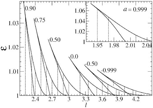
The SA-regions (shocks in accretion) are shown at different spin values for both the standing and dissipative shocks in accretion flows. They are identical and therefore coincide. This implies that the result of Lu & Feng (1997) needs to revised. We see that the region varies significantly with flow parameters (|${\cal E}$|, ł) and black hole spin (a). The angular momentum values are plotted along the vertical dashed lines at (a = 0.999, l = 1.95, 1.97, 2.02), (a = 0.90, l = 2.225, 2.335, 2.4), (a = 0.75, l = 2.5, 2.6, 2.7), (a = 0.50, l = 2.8, 2.9, 3.0), (a = 0.00, l = 3.2, 3.35, 3.5), (a = −0.50, l = 3.6, 3.7, 3.85), (a = −0.999, l = 3.8, 4.0, 4.15) to further study the properties of the dissipative shocks. The parameter a = 0.999 is shown in the subpanel of the figure.
3.3 The nature of the solutions with shocks
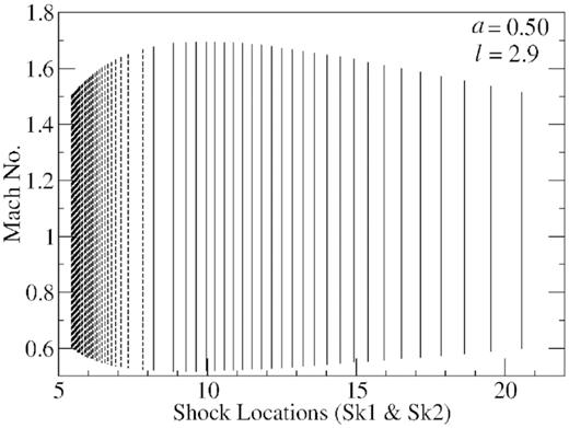
To investigate the nature of the solutions, we integrate the equation |$\frac{\mathrm{ d}v}{\mathrm{ d}r}$| with the help of sonic point conditions and obtain v = v(r). The specific energy and specific angular momentum are chosen from the SA-region for a given spin of the black hole. The solutions also contain three sonic points – inner I (between 3 and 10rg radii), middle M (between 10 and 20rg radii), and outer O (mostly above 20rg radii). The pre-shock and post-shock branches of these solutions now satisfy the Rankine-Hugoniot shock conditions. Moreover, each solution allows a pair of shock solutions corresponding to unstable shock ‘Sk1’ and stable shock ‘Sk2’. The location of Sk1 is formed closer while Sk2 is formed at relatively larger distances in a steady transonic accretion flows. In Fig. 2, locations of an unstable and a stable shocks Sk1 and Sk2 are shown, respectively. We see that Sk1 lies between I and M, while Sk2 lies between M and O sonic points, i.e. on the opposite sides of the middle sonic point M. Thus, from the outer boundary, accretion flows subsonically cross the outer sonic point O and become supersonic. These supersonic flows may jump at Sk1 or Sk2 and become subsonic. The subsonic flows once again cross the inner (I) sonic point to become supersonic and finally reach the inner boundary of the black hole. Note that Sk1 is an unstable, jumps occur at Sk2. The flow parameters and spin parameters are shown in the panel. In Fig. 2, shocks are calculated when the energy of the post-shock and pre-shock branches are the same, i.e. |${\cal E}_+ = {\cal E}_-$|. Therefore, the change in the energy |$\Delta {\cal E} = 0$|, i.e. there is no energy dissipation.
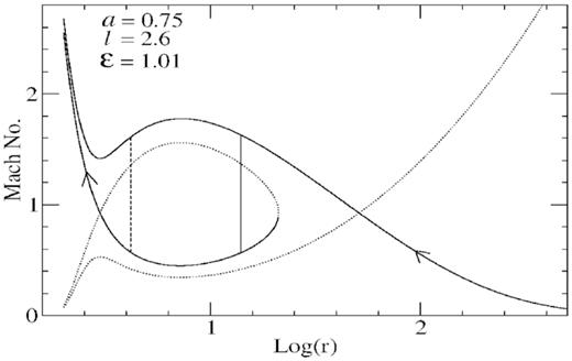
A plot of Mach number versus distance representing the relativistic hydrodynamic solutions with shocks. The locations of an unstable Sk1 (dashed vertical line) and a stable shocks Sk2 (solid vertical line) are shown in the figure in case of non-dissipative shocks. The accretion flows from the outer boundary subsonically cross the outer sonic point to become supersonic. The supersonic flows may jump at Sk1 or Sk2 shock locations to become subsonic. The subsonic flows once again cross the inner sonic point to become supersonic and finally reach the inner boundary of the black hole. Since Sk1 is an unstable location, jumps occur at Sk2.
4 DISSIPATIVE SHOCKS IN ACCRETION FLOWS
Apart from this condition, the other two conditions remain preserved. Note that kinetic energy of the pre-shock flow has already been converted to thermal energy during shock transition. Hence, the thermal energy is the major component of the total energy in the post-shock corona. As a consequence of release of bulk energy |$\Delta {\cal E}$| from post-shock region, pressure drops in the corona. The shock conditions no longer satisfy in its previous location. To maintain the pressure balance between two regions, shock moves forward towards the black hole, compressing the size of the post-shock corona. Therefore, presence of the dissipative shock in accretion disc changes the geometry and hence influences the dynamics of the post-shock corona. Hence the amount of energy release plays as a control parameter in determining the geometry and the dynamics of the corona. We put special emphasis on this feature.
Howeve,r note that we assumed the energy release to be instantaneous, occurring immediately after the shock transition. But the energy release in corona occurs mainly due to Comptonization cooling processes. The process of cooling is highly non-local phenomenon and the energy loss processes are continuous and happen in an extended frequency range. Therefore, in order to obtain the net loss, one has to integrate this emitted spectrum over the whole frequency range.
5 THE STRUCTURE OF DISSIPATIVE SHOCK FRONTS
The structure of the radiative shock front varies crucially depending upon the shock strength and the relative strength of radiation and gas pressure. In most of the cases when the shocks are weak (Compression ratio is <7) or prad < 4.5pgas, the front structure contains discontinuity. The general structure in this case consists of a pre-heating or precursor region, a hydrodynamic compression region (compression shock, denoted by point A in Fig. 3) where flow variables make a sharp transition from pre-shock to post-shock values within a length scale of the order of few molecular mean free path, and a relaxation region (denoted as region II, Fig. 3) where the post-shock matter cools down through radiative processes and through redistribution of energy into the internal degrees of freedom of the constituent fluid particles. At the end of the relaxation zone matter comes into thermodynamic equilibrium and settles in to a steady post-shock solution (point B in our work). The term ‘shock front’ we refer here hydrodynamic compression region (shown in Fig. 3).
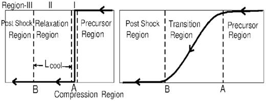
Schematic diagram represents thin (left-hand side) and thick (right-hand side) radiative shocks. AB represents the width of the shock which is of the order of a few photon mean free path. The different regions are shown in the figure (for reference, see also Zeld́ovich & Raizer 1967; Mihalas & Mihalas 1984; Drake 2007). An enlarged hydrodynamic compression region having negligible width of the order of few molecular mean free path is also shown for a thin shock by two vertical dashed lines with a centred solid line at A.
It should be noted that the actual shock compression (compression shock), where the directed (radial) velocities of the fluid elements convert to the random velocities (heat) of the constituent particles of the fluid, occurs within a very thin layer of thickness of the order of few molecular mean free path. Since the fluid dynamical description of the matter is valid only on a length scale several orders of magnitude greater than the molecular mean free path, therefore under this framework a compression shock is strictly a discontinuous transformation. However, the width of the relaxation layer in this case becomes of the order of few photon mean free path. Although the photon mean free path λp could be several orders of magnitude greater than the molecular mean free path, in most of the cases it is negligible compared to the system length scale over which flow variables and the space–time metric vary.
The above description of the front structure is valid as long as the fluid particles transfer their momentum mainly through the collision process among themselves (ZR chap I, section 3 page 75, ‘structure and thickness of weak shock front’; also chap VII and the editor’s note in page 467). However, in the very special case when the shock is extremely strong (ρpost/ρpre > 7, Zeld́ovich & Raizer 1967, Chapter VII, fig. 7.30, equation 7.76) and radiation pressure greatly exceeds the gas pressure (prad/pgas > 4.5, Zeld́ovich & Raizer Chapter VII page 546, Mihalas & Mihalas 1984, page 580, equation 104.92) the fluid particles transfer their momentum mainly through the collisions with photons. It is then possible for the flow variables to make continuous transitions within a length scale of the order of several photon mean free path λp (which is several times greater than the molecular mean free path) as a result the shock becomes thick (dispersed).
For the system we consider here, gas pressure dominates over the radiation pressure (prad < pgas). Also the shock strength is in between moderate to weak (the maximum compression ratio is around 2) and the λp is around 10−2–10−4rg. Therefore, the shock in our case is thin and the shock locations we have shown in the figures refer to the region where hydrodynamic compression shock takes place (region I, point ‘A’). Note that along a given flow branch (a pre- or post-shock steady solution) the flow variables vary non-negligibly only over a length scale of the order of few Schwarzschild radius (rg) (see Figs 2 and 4). This is because gravity is able to impart energy and momentum to the system, only over that length scale. Hence, within the relaxation region flow variables do not change appreciably due to the influence of gravity. However, because this region is extremely hot, radiation flux takes away the energy out of the disc from this region. Note that the radiation flux being c times greater, the radiation energy density has important effect in determining the structure and properties of radiative shock even when radiation energy density (and pressure) is negligible compared to the gas pressure (Mihalas & Mihalas 1984, Chapter 8, page-559).
5.1 Jump Conditions in Radiative Shocks
We would like to emphasize again that energy dissipates from the relaxation layer (region II) and not from the compression shock front (point A). Also the post-shock flow joins a steady post-shock branch at point B (end of the relaxation layer shown in Fig. 3) and not at point A (compression shock front); however, the width AB is negligible (10−4rg) compared to the system length scale.
We write the momentum and energy balance condition between region III (point B where the post-shock fluid joins a steady solution) and the per-shock region. As the thickness of this region is negligible compared to rg (over which metric coefficient typically vary) gravity cannot supply non-negligible amount of energy and momentum to the system. However, radiation flux does carry away energy from this hot region, and one has to consider this while writing the energy and momentum balance condition between points A and B. Although the outgoing radiation carries away energy form the disc, it does not carry away any net momentum since the radiation going out of the disc is emitted symmetrically both in the positive and the negative z-direction. Therefore, the overall momentum flux remains conserved, however, energy flux is not. Hence |$\cal {E}_+ \lt \cal {E}_{-}$| but W+ = W−. Note that these arguments (and hence the equations expressing the energy–momentum balance) are valid irrespective of whether the shock is thin or thick, as long as the width of the radiative shock layer is negligible compared to system length scale.
6 THE ENTROPY CHANGE DURING ENERGY LOSS
In case of dissipative shocks, the energy range |${\cal E}_{\max} \ge {\cal E} \ge {\cal E}_{\min}$| becomes identical with the standing shock. Therefore, SA-regions coincide to each other. This strongly contradicts result of Lu & Feng (1997) and thus the results need to be revised. This is because dissipative shocks release energy and in the limit |${\cal E} \lt {\cal E}_{\min}$|, Rankine-Hugoniot shock conditions do not fulfil. As a result, lower boundaries of SA-regions are the same for both the standing and dissipative shocks. Therefore, at the lower boundary of SA-region where ΔS = Smax occurs, we see |$\Delta {\cal E}=0$| also.
Similarly at the ΔS = 0, energy releases |$\Delta {\cal E}=0$|, occurs at the upper boundary of SA-region for dissipative shocks. This is because ΔS decreases as |$\Delta {\cal E}$| increases. Since, ΔS = 0 and ΔS cannot be reduced further, ΔS < 0 prohibits shock transition, therefore, |${\cal E}={\cal E}_{\max}$| gives the upper boundary of SA-region for dissipative shocks. Hence, we conclude that the effective area of SA-region is the same for both the standing and dissipative shocks. This has also been numerically verified. The SA-regions for both the shocks are plotted in Fig. 1 for different spin parameters.
Further, we find energy dissipation |$\Delta {\cal E}$| has an upper bound. The upper limit of the |$\Delta {\cal E}$| is constrained by the change in entropy in the post-shock flows during the shock transition. For a given energy and angular momentum parameter inside the SA-region ΔS decreases with increase of |$\Delta {\cal E}$|. The maximum increase of |$\Delta {\cal E}$| occurs when ΔS reaches a minimum value, i.e. when ΔS = 0, |$\Delta {\cal E}$| attains maximum. For ΔS < 0, the Rankine-Hugoniot shock conditions do not hold and shocks do not form in the flow. Thus the change in entropy ΔS makes an upper bound |$0 \le \Delta {\cal E} \le \Delta {\cal E}_{cr}$| for the energy loss. The |$\Delta {\cal E}_{cr}$| corresponds to the topmost points on each individual curves in Fig. 6.
7 DYNAMICAL PROPERTIES OF DISSIPATIVE SHOCKS
The dynamical properties of dissipative shocks play an important role in the energy dissipation. In the previous section, a few important properties of dissipative shocks have already been discussed in the context of standing shocks, e.g. energy loss and entropy change. However, to explore the above-mentioned properties for real system, one needs to numerically compute it. In numerical computation we first study the amount of energy loss during the supersonic to subsonic shock transition. As already mentioned, in the presence of a dissipative shock in the flow, |${\cal E}_+ + \Delta {\cal E} = {\cal E}_-$| holds, i.e. energy of the post-shock is less than the pre-shock energy, and |$\Delta {\cal E}$| amount of energy could be dissipated during shock transition. Therefore, we choose the parameters (|${\cal E}, l, a$|) from the SA-region so that hydrodynamic solutions contain two shocks Sk1 and Sk2. Now to find out the energy loss |$\Delta {\cal E}$| in terms of input energy, angular momentum and spin of the black hole, three vertical dashed lines are drawn on each of the SA-regions as shown in the Fig. 1. For a given spin parameter, the values of the angular momentum are chosen in such a way that it admits a very low, a moderately low, and a comparatively high angular momentum. We see that depending on the angular momentum values, small, moderate, and large energy ranges occur between the boundaries of a SA-region. The energy values are chosen from the upper and lower boundaries of an SA-region along these vertical lines. Depending on the span of the lines, we choose energy resolution of the order of 10−5–10−4 in the numerical codes. Since Fig. 1 contains SA-regions for seven black hole spin parameters including co- and contra-rotation, three different angular momentum values on each SA-region means total 21 sets of parameters are considered to investigate the energy dissipation during shocks. These sets are: (a = 0.999, l = 1.95, 1.97, 2.02), (a = 0.90, l = 2.225, 2.335, 2.4), (a = 0.75, l = 2.5, 2.6, 2.7), (a = 0.50, l = 2.8, 2.9, 3.0), (a = 0.00, l = 3.2, 3.35, 3.5), (a = −0.50, l = 3.6, 3.7, 3.85), and (a = −0.999, l = 3.8, 4.0, 4.15). All the 21 sets of parameters are shown in Fig. 1. Since the SA-region corresponding to a = 0.999 is small, it has been highlighted separately in the subpanel.
Taking one (|${\cal E}, l, a$|) within this sets of parameters, we obtain the solution topology containing supersonic branch having in-fall energy |${\cal E}={\cal E}_-={\cal E}_{in}$| (say). As already stated, in the case of dissipative shock, energies of the pre-shock and post-shock flows are not same. Therefore, for a given in-flow energy, shock transitions are possible between the pre-shock branch and different post-shock branches. Since the dissipated energy |$\Delta {\cal E}={\cal E}_{in}-{\cal E}_+$|, for a fix energy of the incoming flow dissipated energy |$\Delta {\cal E}$| may vary.
As a result of energy release pressure drops, both the shock locations Sk1 and Sk2 will form in a new location in order to maintain the pressure balance. With the increasing |$\Delta {\cal E}$|, pressure drop increases hence to maintain the pressure balance condition Sk2 shifts at smaller radii and Sk1 shifts at higher radii. So the two shocks approach to each other and may merge together for sufficiently high value of |$\Delta {\cal E}$|. Therefore, there exist a critical value of |$\Delta {\cal E}=\Delta {\cal E}_{cr}$| at which both the shocks Sk1 and Sk2 merge to a single point. No further shock forms in the flows for |$\Delta {\cal E} \gt \Delta {\cal E}_{cr}$|. Therefore, |$\Delta {\cal E}_{cr}$| is the maximum value of dissipated energy for a given |${\cal E}_{in}$|. For the different values of inflow energy |${\cal E}_{in}$|, the values of |$\Delta {\cal E}_{cr}$| are different. The amount of |$\Delta {\cal E}_{cr}$| therefore depends on the (i) specific energy (|${\cal E}_{in}$|) of the incoming pre-shock flow, (ii) specific angular momentum (l) of the flow, and (iii) the spin parameter (a) of the black hole, i.e, |$\Delta {\cal E}_{cr} = \Delta {\cal E}({\cal E}_{in}, l, a)$|.
In Fig. 4, we show how the stable shock location Sk2 change with the increase of dissipated energy |$\Delta {\cal E}$|. Depending on the different values of |$\Delta {\cal E}$| the different post-shock branches are shown. As |$\Delta {\cal E}$| increases Sk2 moves inwards to maintain the Rankine-Hugoniot shock condition between the supersonic and successive subsonic branches. In the figure, we see that the changes in the post-shock branches are small. This is because an insignificant change occurs in the location of the inner sonic point (I) due to |$\Delta {\cal E}$|.
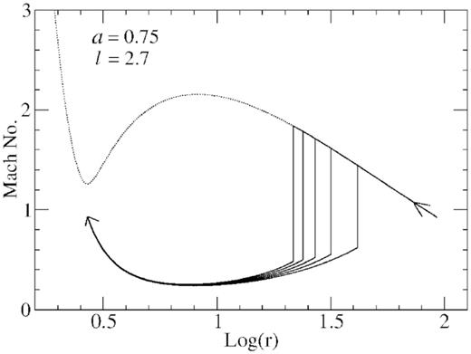
We show the variation of shock locations Sk2 as a function dissipated energy at different steps. Sk2 moves towards the black hole as the energy dissipation increases. We see that a very small change in the post-shock branches can introduce a large change in the stable shock location Sk2. The shape and size of the post-shock corona changes as the shock boundary moves inward.
However, a small change in the post-shock branches introduces a large change in the stable shock location Sk2 and comparatively much smaller changes in the unstable shock location Sk1. In Fig. 5, we plot the various locations of the both the shocks Sk1 (dashed) and Sk2 (solid) in different steps with the increasing values of |$\Delta {\cal E}$|. We see that as |$\Delta {\cal E}$| increases both the shocks Sk1 and Sk2 move towards 8rg where middle sonic point is located; however, shift in the position is more for Sk2 in comparison with the Sk1. Finally, both Sk1 and Sk2 merge close to the middle sonic point and then get disappeared for a particular value of |$\Delta {\cal E}$| known as |$\Delta {\cal E}_{cr}$|. Beyond |$\Delta {\cal E}_{cr}$|, no shock forms in the flow. Therefore, |$\Delta {\cal E}_{cr}$| is the maximum possible value of the dissipated energy for the inflow parameter |$({\cal E}_{in}, l, a)$|.
We show how the shock locations Sk1 (dashed) and Sk2 (solid) vary with the increase of energy loss |$\Delta {\cal E}$|. We see that both Sk1 and Sk2 merge close to the middle sonic point and finally disappear when |$\Delta {\cal E}$| reaches a critical value. Therefore, the corona geometry changes according to the radiative loss of energy from it.
7.1 Energy loss from the corona
Since the maximum energy dissipation |$\Delta {\cal E}_{cr}$| is a function of |$({\cal E}_{in}, l, a)$|, therefore keeping spin parameter a and angular momentum l fixed, we change the energy |${\cal E}_{in}$| of the pre-shock branch. That means we chose another neighbourhood point on the same vertical line in the SA-region. We then calculate the shock locations in different numerical steps with |$\Delta {\cal E}$| as a parameter and estimate |$\Delta {\cal E}_{cr}$|. We find that different values of inflow matter dissipate different amount of |$\Delta {\cal E}_{cr}$|. Note that |$\Delta {\cal E}_{cr}=0$| in both the boundaries of SA-region. Therefore, the value of the energy |${\cal E}_{in}$| for which |$\Delta {\cal E}_{cr}$| is maximum corresponds to a point well inside the SA-region. Following the same process, the variation of |$\Delta {\cal E}_{cr}$| with the |${\cal E}_{in}$| as parameter is investigated to obtain the extremum energy dissipation. For a given l, we choose different inflow energy |${\cal E}_{in}$| starting from the top most point and ending at the bottom of the lower boundary of the SA-region, we calculate a series of |$\Delta {\cal E}_{cr}$| values. Comparing the magnitude of |$\Delta {\cal E}_{cr}$|, we determine the maximum value |$\Delta {\cal E}_{\max}$|. Therefore, for a given angular momentum l and spin parameter a, the |$\Delta {\cal E}_{\max}$| represents maximum amount of energy dissipation that may be emitted as E.M radiation from the post-shock corona.
In Fig. 6, we plot the variation of |$\Delta {\cal E}$| with the inflow energy |${\cal E}_{in}$| for a given angular momentum l and spin parameter a. Different curves are plotted for different initial energies |${\cal E}_{in}$|. We see that when inflow energy is high, in particular close to the upper boundary of the SA-region, dissipation of |${\cal E}$| is small. The magnitude of |$\Delta {\cal E}$| increases initially with the decrease of initial energy |${\cal E}_{in}$|, reaches a maximum value and then decreases with the further decrease of initial energy. The energy |${\cal E}_{in}$| at which dissipated energy |$\Delta {\cal E}$| reaches its maximum, could also be estimated directly from the figure. Therefore, for a given angular momentum and spin of the black hole, the tallest line denote maximum value of the energy emission which could be possible to dissipate from the post-shock region.
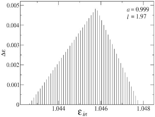
We plot the variation of energy loss |$\Delta {\cal E}$| from post-shock corona with the inflow energy |${\cal E}_{in}$| of the pre-shock matter. We see that energy loss |$\Delta {\cal E} \rightarrow 0$| at both ends of the upper and lower boundaries of SA-region. The energy loss increases with the decrease of energy |${\cal E}_{in}$| initially. It reaches a maximum value and then again decreases. The magnitude of |$\Delta {\cal E}$| is plotted in the energy range between the upper and lower boundaries of the SA-region.
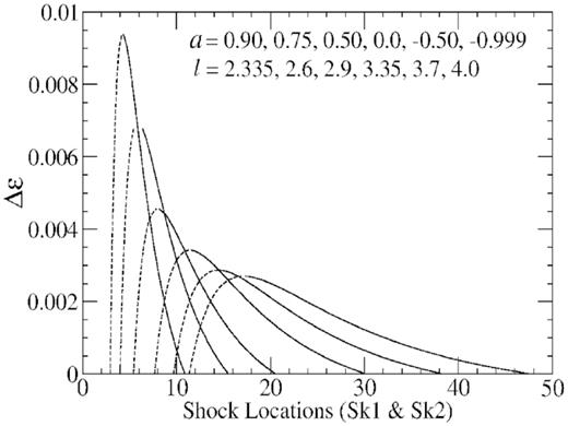
Since, the maximum values of the dissipated energy |$\Delta {\cal E}_{\max}$| also depends on the angular momentum l of the flow and the spin parameter a of the black hole, therefore keeping spin parameter a fixed, we plot |$\Delta {\cal E}$| versus inflow energy |${\cal E}_{in}$| at three different values of angular momentum l and compare the peak values in Fig. 7. In the plot, different peaks are presented in which l values decreases from left to right. We see that for low and high angular momentum, say l = 3.2, 3.5, peaks are low and become maximum at an intermediate values of the angular momentum l = 3.35. Interestingly in case of high angular momentum (see the figure for l = 3.5), the dissipative curves at low energies |$\Delta {\cal E}$| become almost equal to |$({\cal E}_{in}-1)$|, i.e. reaches close to |$100{{\ \rm per\ cent}}$|. Note that |${\cal E}_{in}-1$| is the total energy minus the rest mass energy which is equals to thermal, kinetic and potential energy. Therefore, our observations suggest that the magnitude of the dissipated energy become maximum at an intermediate value of angular momentum. But the percentage of energy dissipation become maximum at high angular momentum and at low energy.
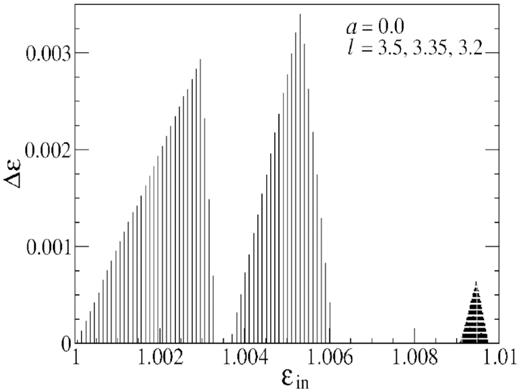
We plot |$\Delta {\cal E}$| with respect to inflow energy |${\cal E}_{in}$| at three different values of angular momentum l to compare losses. We see that maximum energy loss occurs at intermediate angular momentum values. Therefore, the amount of energy loss fully depends on the flow parameters.
7.2 The corona size with energy loss
As already been stated, increase of energy loss results in decrease of post-shock pressure hence to maintain the equilibrium across the boundary shock propagate towards a smaller radii. Therefore corona size decreases. We study the connection between energy loss and corona size. A plot is also shown in Fig. 8, where we calculate |$\Delta {\cal E}$| in terms of the locations of the propagating shock Sk2. In the absence of the dissipation, the initial location of Sk2 depends on |${\cal E}_{in}$| therefore, at high |${\cal E}_{in}$|, Sk2 occurs at large r while at low energies shocks come closer. Thus in the nearby points of upper boundary of the SA-region, shocks form at larger radii. With the decrease of |${\cal E}_{in}$| shocks form at relatively smaller radii, |$\Delta {\cal E}$| increases. Finally, |$\Delta {\cal E}$| attends maximum for a particular curve and after that peak decreases. We find that |$\Delta {\cal E}$| attains a maximum value near the upper boundary of the SA-region. The values of |$\Delta {\cal E}_{\max}$| depends on the (a, l) pair. At low energies peaks of all Sk2 curves reach a minimum value (near about at 5rg in figure) and then disappear from there (a point close to the middle sonic point). Note that in general the variation of the middle sonic point is small at low l and moderate at high l values. Therefore in the subpanel of the figure, we see that Sk2 disappear at different radii (left-hand side of the figure) depending on the position of the middle sonic point.
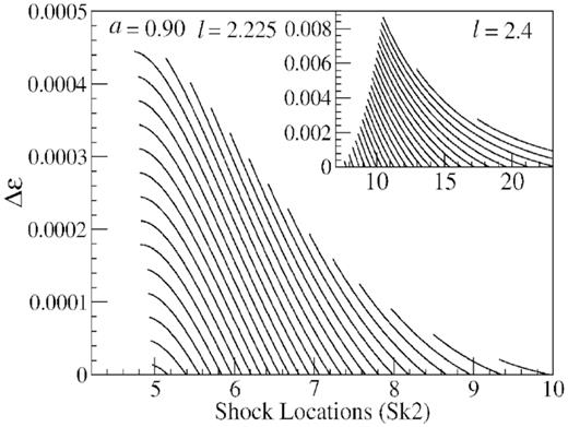
The variation of energy loss |$\Delta {\cal E}$| is presented as the function of the shock location Sk2. It moves towards the inner edge of the disc. The |$\Delta {\cal E}$| attends maximum for a particular curve with a definite values of |${\cal E}_{in}$|. We see that there is a lower cut-off of Sk2 at 5rg (near about the middle sonic point for a = 0.90) which is generally observed at low energies. Therefore, radii of corona decrease with the energy loss. The lower cut-off provides minimum size of the corona when all of its energy being dissipated out.
7.3 Efficiency of coronal emission
At this point we will investigate the efficiency of the coronal emission. At the low energies, we find the magnitude of the energy dissipation is small. However, dissipation of the fluid energy (excluding its rest mass energy) with respect to its total energy is high. Therefore, the percentage of energy dissipation could reach close to |$100{{\ \rm per\ cent}}$|. To see that we plot the percentage of the energy dissipation |$\Delta {\cal E}/({\cal E}_{in}-1)$| with respect to the Sk2 in Fig. 9. Since the rest mass energy is subtracted from the total energy, |$({\cal E}_{in}-1)$| is now equal to the sum of the kinetic, thermal and gravitational energy. A major part of this energy can be dissipated out from the system during shock transition. Thus, mostly at the low energies and at high angular momentum values, we compare the percentage of the energy dissipation. In the figure, we see that at l = 2.335 (low angular momentum), |$\Delta {\cal E}/({\cal E}_{in}-1)$| is around |$65{{\ \rm per\ cent}}$|, shown in the sub-panel, whereas at comparatively high angular momentum l = 2.4, |$\Delta {\cal E}/({\cal E}_{in}-1)$| is close to |$100{{\ \rm per\ cent}}$|. One such solution topology having different dissipated energy at different steps is presented in Fig. 10. Here we clearly see that as Sk2 moves towards the black hole as the percentage of dissipated energy is increased significantly and becomes close to |$100{{\ \rm per\ cent}}$| (see also the subpanel). It means flow may dissipate out almost all of its kinetic, thermal and gravitational energy, only rest mass energy remains. Hence the efficiency of the coronal emission is high. As a result of that, energy gets exhausted, only rest mass energy remains in the flow. The implication of this could be profound because a significant portion of the bulk energy may get dissipated from the post-shock corona. The emission of hard X-rays from the inner edge of the disc may take place due to such amount of energy release.
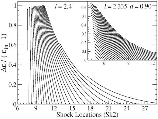
The fractional of the energy dissipation |$\Delta {\cal E}/({\cal E}_{in}-1)$| with respect to the Sk2 is presented. At high angular momentum l = 2.4, |$\Delta {\cal E}/({\cal E}_{in}-1)$| reaches close to |$100{{\ \rm per\ cent}}$|. It means that depending on the flow parameters, flow can dissipate out almost all of its kinetic and thermal energies, only rest mass energy remains.
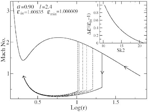
We show the variation of shock location Sk2 as a function dissipated energy at different steps. Sk2 moves towards the black hole as the energy dissipation increases. The percentage of the energy dissipation |$\Delta {\cal E}/({\cal E}_{in}-1)$| with respect to the Sk2 is shown (see the subpanel also). At l = 2.4, |$\Delta {\cal E}/({\cal E}_{in}-1)$| reaches close to |$100{{\ \rm per\ cent}}$|. It means that depending on the flow parameters, flow can dissipate out almost all of its energy, only rest mass energy remains.
8 THE VARIATION OF SPECTRAL PARAMETERS WITH ENERGY LOSS
The spectral variabilities of accretion disc are mostly studied from the variation of the hydrodynamic and thermodynamics quantities with respect to the temperature and radii of the of post-shock corona. Until now we have studied the variation of |$\Delta {\cal E}$| with respect to the energy |${\cal E}_{in}$| and shock locations Sk1 and Sk2, which in turn helps us to find out the maximum possible energy dissipation during pre-shock to post-shock transition. However, there are several other interesting aspects of the dissipative shocks which could be studied. Among them one of the important quantity is the strength of the shock which is determined by the amount of entropy change during shock transition. The information about the gain in entropy during pre-shock to post-shock transition, has been nicely inbuilt in one of the hydrodynamic variable so-called ‘entropy accretion rate(S)’, defined as |$S=\dot{\cal {M}} = K^{n}\gamma ^{n}\dot{M}$|. Here |$\dot{M}$| is mass flux and the constant K is measure of the entropy because K satisfies the adiabatic equation of state |$P = K{\rho _{0}^{\gamma }}$|. The amount of change of the flow entropy is now measured through the parameter S during shock transition. For the entire set of parameters (|${\cal E}, l$|) chosen from SA-region, ΔS ≥ 0. Introduction of the dissipative shocks in the accretion flows in which a part of the flow energy being expelled out from the system, generates less amount of entropy gain ΔS and hence produces a weaker shock strength. With the increase of |$\Delta {\cal E}$|, the strength of the shock become more and more weaker. This dynamical property of the dissipative shocks is nicely being captured in Fig. 11, in which we plot the entropy accretion rate(S) versus the shock locations Sk1 and Sk2 at different |$\Delta {\cal E}$|. The solid vertical line represents the change in entropy accretion rate (S) at the location of Sk2 while dashed vertical line represents the change in entropy accretion rate (S) at the location of Sk1. The upper-most and lower-most points of a particular straight line corresponds to the entropy of pre-shock and post-shock branch respectively. It can be seen from the plot that entropy of the post-shock branches have higher value than the corresponding pre-shock branches. In our plot the energy of the pre-shock branch is taken to be same therefore the points at the bottoms of the vertical lines lie on a horizontal straight line. As both Sk2 (solid) and Sk1 (dashed) move closer to each other, the length of the vertical line decreases significantly, indicating the fact that the gain of entropy during shock transition decreases. Therefore, the strength of the shocks become more and more weaker as |$\Delta {\cal E}$| increases. At the point where both the shocks merge together and disappear, the strength of the shock become weakest as shown in figure close to 5rg.
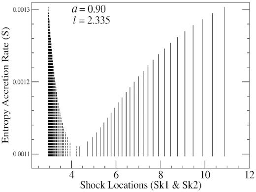
We plot the change in entropy accretion rate(S) versus the shock locations Sk1 and Sk2 at different |$\Delta {\cal E}$|. As both Sk2 (solid) and Sk1 (dotted) shocks merge towards each other, we see that length of the vertical line decreases, indicating the change in entropy during shock transition also decreases towards zero value. Therefore, shocks become more and more weaker as |$\Delta {\cal E}$| increases. Therefore, the total amount of energy loss from the corona is constrained by the entropy change during shock transition.
Moreover, the location and strength of the dissipative shock play an important role to determine the geometry and spectral properties of the accretion disc. Shock creates a boundary layer and separates the hot post-shock corona from the pre-shock flow having low temperature. With the increase of energy dissipation, shock moves inwards, the size of post-shock corona thus decreases. However, strength of the shock reduces. The spectral variation and its properties therefore can be determined by the size of the post-shock corona, temperature difference (ΔT), compression ratios, etc. Keeping that in mind, we further study the temperature generation in the post-shock region during shock propagation.
8.1 The coronal temperature variation
The variation of temperature in the post-shock corona solely depends on the entropy generation in the post-shock flows during shock propagation. Therefore we study the relation between entropy generation and temperature variation in the post-shock flows. To do that we investigate the variation of the ratios of the post-shock to pre-shock entropy accretion rate (S+/S−) and temperature (T+/T−), when shock propagates. We plot them with respect to the stable shock locations Sk2 in Figs 12 and 13 respectively. At low angular momentum, shown in the sub-panel of Fig. 12, we see that ratios of the S+/S− decreases as shocks move inward. When the shock locations are comparatively at large radii (curves at the right) the ratio S+/S− tends to 1. The decreasing tendency of the ratio S+/S− as shock moves inwards is also present for high angular momentum (l = 2.4) but the fractional change of S+/S− is insignificant. The almost similar behaviour is observed for the temperature ratios (T+/T−). For both the low and high angular momentum, the fractional change of (T+/T−) increases slightly as shock moves inwards however the amount of change is insignificant in this case too. The variation pattern of both the ratios S+/S− and (T+/T−) are quite similar, this is expected as the entropy is a function temperature.
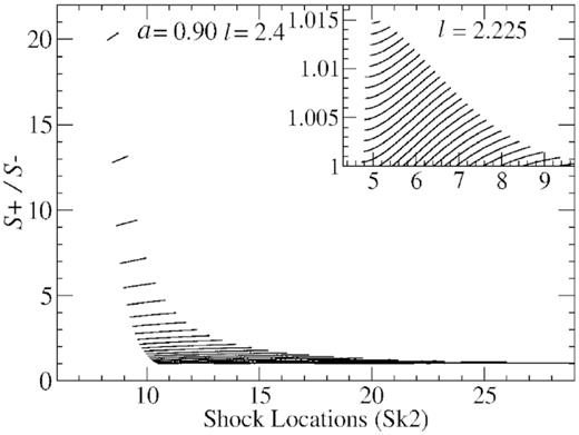
The variation of the ratios of the post-shock to pre-shock entropy accretion rate (S+/S−) is shown with respect to the stable shock location Sk2. We see that ratios of the S+/S− decrease as Sk2 moves inward but the change is small with respect to the initial ratio.
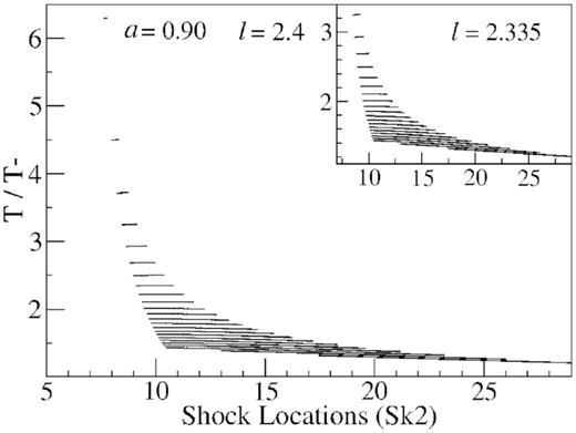
The variation of the ratios of the post-shock to pre-shock temperature (T+/T−) is presented with respect to the stable shock location Sk2. The overall variation of both the ratios S+/S− and (T+/T−) is quite similar, since the entropy is a function temperature.
We further investigate the percentage change in temperature ΔT/T+ in the post-shock corona zone. In Fig. 14, we plot ΔT/T+ with respect to shock locations. From the figure we see that with the decrease in shock location, the percentage change in temperature ΔT/T+ increases. It attains a maximum at some intermediate values where |$\Delta {\cal E}$| is maximum. However the percentage change ΔT/T+ is not much and lies within |$1{{\ \rm per\ cent}}$| to |$2{{\ \rm per\ cent}}$|. This behaviour is quite evident in spectral variations also. As the radii of corona shrink, the temperature remains fixed initially. It generally falls off due to the mass loss when jet is formed. Therefore, by studying energy loss, the change in the hydrodynamic and thermodynamics variables with respect to the change in temperature and radius of the of post-shock corona we get some insight which are required to investigate the spectral variabilities of the accretion discs.
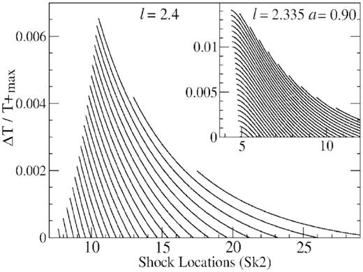
We plot ΔT/T+ as a function of shock location Sk2. As shock location moves inwards, corona size reduces. The percentage change in temperature ΔT/T+ is also increases. It attains a maximum at some intermediate values. However the fractional change in temperature lies between |$1{{\ \rm per\ cent}}$| and |$2{{\ \rm per\ cent}}$|.
8.2 The compression ratio
We have already noticed that the corona gets compressed as the shock moves inward. Therefore, the compression ratio needs to be investigated. The strength of the shock also determined by the compression ratio. In Fig. 15, we plot the compression ratio ‘Rcomp’ as a function of the shock location for different inflow energies. When dissipation is increased, the compression ratio increases linearly as Sk2 moves inward. However with respect to its initial values the fractional change is small. For low angular momentum (as shown in the subpanel) the compression ratio although increases initially, decrease slowly later. However, so far in most of the theoretical studies (Chakrabarti et al. 2009) it being assumed that compression ratio gradually decreases as corona size reduces, but our investigation reveals that the variation is reversed. This is because they have used the properties of standing shocks. But without a detail analysis of the dynamical properties of the dissipative shocks, a correct variation of the compression ration cannot be obtained only by studying the properties of standing shocks.
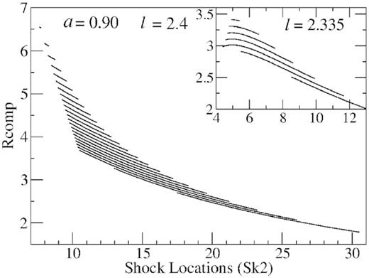
The compression ratio is plotted when shock moves inward at different inflow energy. The compression ratio increases linearly but with respect to its initial values, the change is small. In the subpanel, the compression ratio increases initially but slowly decrease at the end for low angular momentum values. It is important to note that in the observational studies it is assumed that compression ratio gradually decreases as corona size reduces, however, a theoretical investigation reveals that the variation is reversed.
9 BLACK HOLE SPIN AND ENERGY RADIATION
Finally, we concentrate our attention on the issue of the dependence of the coronal energy dissipation from black hole spin. We consider several spin parameters ranging from a = −0.999 to a = 0.90. To compare the magnitude of the dissipation energy |$\Delta {\cal E}$|, a large set of flow parameters is considered from the SA-region at different spins. For a given pair of (a, l) value we computed |$\Delta {\cal E}$| for various values of |${\cal E_{in}}$| and picked up the curve corresponding to the maximum value of the |$\Delta {\cal E}$|. One such plot is presented in Fig. 8. The variation of |$\Delta {\cal E}$| with respect to both the shock locations Sk1 (dashed) and Sk2 (solid) is shown in Fig. 16. The values of spin parameter a and l is printed from left to right of the figure panel. We see that the location of Sk2 (solid) shifts inwards while Sk1 (dashed) shifts out wards as |$\Delta {\cal E}$| increases. The peak of the curves where both the shock locations Sk1 and Sk2 merge together close to middle sonic point, increases with the spin of the black holes. We observe the variation in the entire range of the spin parameter −0.999 ≤ a ≤ 0.999. We plot spin parameter −0.999 ≤ a ≤ 0.90 because the peak become much higher at a = 0.999. Hence, it is clear that coronal energy dissipation gets significantly enhanced by spin of the black hole.
We replot the curves for which the energy dissipation is maximum in the flows for all sets of (a, l) pairs. The values of spin parameters a and l are printed from left to right of the figure. We see that when both the shock locations Sk1 (dashed) and Sk2 (solid) merge together near the middle sonic point, the energy dissipation becomes maximum. The energy loss increases with the increase of the spin parameter a from −0.999 to 0.90.
The maximum amount of dissipated energy in terms of |$\Delta {\cal E}/{\cal E}_{in}$| is also plotted in Fig. 17, as a function of inflow energy for different angular momentum l and same spin parameters a. The value of |$\Delta {\cal E}/{\cal E}_{in}$| gives the percentage of dissipated energy with respect to the total energy. From the height of the several solid vertical lines, plotted in the figure, we see that as the spin parameter increases, the value of |$\Delta {\cal E}/{\cal E}_{in}$| also increases and become maximum at a = 0.90. We also checked for a = 0.999 and find that the peak value is much higher. Therefore, we can conclude that energy dissipation from the post-shock corona gets greatly enhanced by the co-rotating spins of the black hole. The effect is reversed in case of contra-rotating black holes.
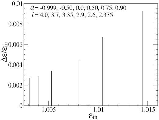
The fraction of dissipated energy |$\Delta {\cal E}/{\cal E}_{in}$| is plotted as a function of inflow energy |${\cal E}_{in}$| for different values of a, ł pairs printed left to right successively. We see that as the spin parameter is increased the value of |$\Delta {\cal E}/{\cal E}_{in}$| is also increased. Therefore, the energy dissipation from the post-shock corona gets greatly enhanced by the co-rotating spins of the black hole. The effect is reversed in case of contra-rotating black holes.
10 QPOS AND SHOCK OSCILLATIONS
In this section, as an application, we try to relate the effect of oscillating shocks to observed QPO phenomena. The QPO oscillations are believed to be originated due to the oscillations of the disc under small perturbations. In the common approach, the oscillation frequencies are obtained by perturbing the Keplerian orbit of a particle. They are: Keplerian orbital frequency νK = ΩK/2π, radial epicyclic frequency νr = ωr/2π, and vertical epicyclic frequency νν = ων/2π. Here the expressions of ΩK = 1/(r3/2 + a), |$\omega _r^2=\alpha _r\Omega _K^2$|, |$\omega _r^2=\alpha _{\nu }\Omega _K^2$|, where αr = 1 − 6r + 8ar−3/2 − 3a2r−2, and αν = 1 − 4ar−3/2 + 3a2r−2 are given for the disc orbiting Kerr black holes (Kato & Fukue 1980; Okazaki et al. 1987; Nowak & Lehr 1999). However, this approach is acceptable for the disc for which the fluid matter follows the Keplerian orbit (e.g. Shakura and Sunyaev disc). But in the real systems the disc may not be Keplerian always.
The presence of the dissipative shock can also excite QPO phenomena. This is because as the dissipative shock propagates inwards, energy dissipates, which can create instabilities resulting the boundary layer of the post-shock corona to oscillate. These oscillations may excite QPOs in hard X-rays. Note that this is purely a hydrodynamical phenomenon and has to be studied by perturbing the original fluid dynamical equations. The study of the disc perturbations through this approach have been done by quite a few authors (Silbergleit et al. 2001; Stella & Vietri 1999; Abramowicz & Kluźniak 2001; Klúzniak & Abramowicz 2001; Abramowicz et al. 2003; Rezzolla, Yoshida & Zanotti 2003; Kato 2004; Kluźniak et al. 2004; Qian & Wu 2005; Blaes, Arras & Fragile 2006; Horák 2008; Fragile et al. 2016; Dewberry et al. 2018). In general it has been found that QPO frequency obtained in this way are close to the epicyclic frequencies. However, whether the oscillations frequencies bear all the characteristics of the observed QPO frequencies that is theoretically still an open question addressing which is beyond the scope of this work.
However, note that the hydrodynamic solutions presented in our work provide the theoretical inputs required to estimate above disc oscillation frequencies. In addition, from the inputs of the systematic evolution observed QPOs (e.g. XTE J1550−564 and GRO J1655−40 etc.) may also put some constrain on the shock propagation and disc oscillation frequencies, hence the energy release. Thus, by connecting shock oscillation frequency to the observed QPO frequency, one may try to get an observational signature of such oscillating shocks. This work provides a theoretical feedback to answer this question.
11 CONCLUSION
In this paper, we present the dynamical properties of dissipative shocks in accretion flow under the general relativistic frame work. The outcomes of this paper are significantly different from that found in the previous work (Das et al. 2010). One of the main reasons is that they used a pseudo-Newtonian geometry instead of exact relativistic formalism. On the contrary, our results are exact and free from any approximation.
As the dissipative shock removes a significant part of the bulk energy from the post-shock corona, the post-shock pressure decreases. As a result, the shock moves inwards and, therefore, compresses the size of the post-shock corona. This enhances the corona temperature and the compression ratio. Therefore, in the rising phase of the outburst when shock moves inwards, the variation of the hydrodynamical and thermodynamical variables is investigated with respect to the corona size and energy loss. The result of our study would be useful to explain the nature of the EM spectrum that is coming out of the accretion disc.
The temporal variation and spectral properties generally depend on the corona size and energy loss processes. Therefore, we estimate the total energy loss from the corona and calculate the percentage of energy loss. We noticed that for some set of parameter values, total amount of energy dissipation is significantly high. Flow can dissipate almost all its thermal, kinetic, and gravitational energy in the emission processes. The percentage of energy dissipation can reach in principle to a very high value almost close to |$100{{\ \rm per\ cent}}$|. This indeed increases effectiveness of the loss processes in the corona region. The implication of this could be useful to understand the emission of hard X-rays from the inner edge of the disc where a huge amount of bulk energy release takes place.
Moreover, the propagation of the dissipative shocks may also generate oscillations inside the boundary layers, which can excite the QPOs in the emitted X-ray radiation. A systematic evolution of QPOs in their rising phase of the outbursts also indicates that the shock actually propagates towards the black hole. Hence, from the knowledge of the variations of coronal size and energy release the phenomena such as QPOs, time lags between hard and soft X-ray photons, observed in several black hole candidates, could be nicely explained with the help of dissipative shocks.
Further, we study the spin dependence and found that the spin has profound effect on the energy dissipation. The highly co-rotating black holes are more efficient and can emit high amount of energy whereas contra-rotating black holes are less efficient in releasing bulk energy.
As a passing remark, the inspiring proposal of ASTROSAT gives the present research activity a welcome boost in all corners of astrophysics. Since its launch, ASTROSAT has brought lots of new observational features from black holes and several groups are analysing data to extract physics out of it. Therefore, a proper theoretical model of accretion discs is required to explain the outcome from this analysis. The issue of energy dissipation from the inner edge of the disc (where Compton cloud is located) thus becomes very important in the context of current status of accretion physics.
ACKNOWLEDGEMENTS
Authors acknowledge Prof. S. K. Chakrabarti of Indian Centre for Space Physics (ICSP) for useful discussions and thank to Inter-University Centre for Astronomy and Astrophysics (IUCAA), Pune for their support through ‘Visiting Associateship Program’. Also, authors thank to anonymous reviewer for the critical review which helped to improve the quality of the paper.
DATA AVAILABILITY
Data shearing may not be applicable or may not be necessary to this article as it is mostly a theory-based article. No new data set were analysed during this study. The numerically created data that support the findings of this study are available from the corresponding author, upon reasonable request.
