


ABSTRACT
We present detailed spectroscopic analysis of the extraordinarily fast-evolving transient AT2018kzr. The transient’s observed light curve showed a rapid decline rate, comparable to the kilonova AT2017gfo. We calculate a self-consistent sequence of radiative transfer models (using tardis) and determine that the ejecta material is dominated by intermediate-mass elements (O, Mg, and Si), with a photospheric velocity of ∼12 000–14 500 |$\rm {km}\, s^{-1}$|. The early spectra have the unusual combination of being blue but dominated by strong Fe ii and Fe iii absorption features. We show that this combination is only possible with a high Fe content (3.5 per cent). This implies a high Fe/(Ni+Co) ratio. Given the short time from the transient’s proposed explosion epoch, the Fe cannot be 56Fe resulting from the decay of radioactive 56Ni synthesized in the explosion. Instead, we propose that this is stable 54Fe, and that the transient is unusually rich in this isotope. We further identify an additional, high-velocity component of ejecta material at ∼20 000–26 000 |$\rm {km}\, s^{-1}$|, which is mildly asymmetric and detectable through the Ca ii near-infrared triplet. We discuss our findings with reference to a range of plausible progenitor systems and compare with published theoretical work. We conclude that AT2018kzr is most likely the result of a merger between an ONe white dwarf and a neutron star or black hole. As such, it would be the second plausible candidate with a good spectral sequence for the electromagnetic counterpart of a compact binary merger, after AT2017gfo.
1 INTRODUCTION
The advent of wide-field surveys and rapid multiwavelength follow-up has produced discoveries of transients with much faster evolving light curves and spectra than the normal 56Ni powered Type Ia and Ibc population (Poznanski et al. 2010; Drout et al. 2013; De et al. 2018; Prentice et al. 2018,2020; Chen et al. 2020). The nature of these unusual transients is much debated and while many are explosions of a single star (albeit with a binary companion that influences the preceding evolution), some fraction may be violent stellar mergers. Extensive theoretical effort has been invested in exploring the mergers of compact objects, and binary combinations of white dwarfs (WDs), neutron stars (NSs), and stellar mass black holes (BHs) have all been computationally explored in various scenarios (Fryer et al. 1999; King, Olsson & Davies 2007; Fernández, Margalit & Metzger 2019; Metzger 2019). Binary BH mergers are being discovered by LIGO–Virgo at a rate of one per week (Abbott et al. 2016, 2019), a candidate NS–BH merger has been discovered (s190814bv; The LIGO Scientific Collaboration & the Virgo Collaboration 2019), and detections of two binary NS mergers have been published (Abbott et al. 2017a, 2020). Only one compact binary merger, which produced the signal GW 170817, has been unambiguously linked to an electromagnetic signal (Abbott et al. 2017b). Since WDs have radii that are ∼200–700 times larger than NS radii and Schwarzschild radii of 10 M⊙ BHs, a binary merger with a WD component will radiate gravitational waves at frequencies below the LIGO–Virgo detectable range.
There are no confirmed electromagnetic transients of WD–NS or WD–BH mergers to date. However, there is observational evidence for the progenitor binary systems existing. Miller-Jones et al. (2015) and Bahramian et al. (2017) present observational evidence for a candidate WD–BH binary system in the Galactic globular cluster 47 Tucanae. Theory predicts that these mergers are likely to be luminous (Metzger 2012; Margalit & Metzger 2016; Fernández et al. 2019) and detectable in contemporary wide-field surveys. Zenati, Bobrick & Perets (2020) predict somewhat fainter and redder optical transients than Metzger (2012), Margalit & Metzger (2016), and Fernández et al. (2019), but still comfortably within the sensitivity of the Zwicky Transient Facility (ZTF; Bellm et al. 2019) and the Asteroid Terrestrial impact Last Alert System (ATLAS; Smith et al. 2020) in the local Universe. The calculated rates of compact mergers with a WD component suggest they could be as high as 3–15 per cent of the Type Ia rate (Toonen et al. 2018). With a discovered Type Ia rate of ∼90 yr−1 within 100 Mpc (Smith et al. 2020), such a high rate would imply there should be 2–13 such events per year, within this Local Volume. Given that compact binary mergers have been detected through gravitational wave (GW) signals, and the large theoretical rate of mergers with a WD component, it is surprising that there are no obvious candidates from the wide-field surveys. Significant computational work has also been published on the merger of WDs with intermediate-mass BHs (Rosswog, Ramirez-Ruiz & Hix 2009; MacLeod et al. 2016), but no convincing candidate has yet been identified.
The most reliable method of determining the chemical composition of an astrophysical transient is by analysing its spectra with radiative transfer methods. From spectral modelling, one can aim to deduce the composition of the spectral-forming region. This information is invaluable when it comes to determining the progenitor system, and understanding the physical nature of an explosive transient. The open source radiative transfer code tardis (Kerzendorf & Sim 2014; Kerzendorf et al. 2019) is now applied to model spectral sequences of both Type Ia and Type II supernovae (SNe; Vogl et al. 2020). For Type Ia SN, it has been used to determine the ejecta composition of Type Iax SNe to aid understanding of the explosion mechanisms (Magee et al. 2016; Barna et al. 2017), and to constrain the existence of He in double detonation scenarios (Boyle et al. 2017).
In this paper, we present a detailed spectroscopic analysis of AT2018kzr, a remarkably fast declining transient jointly discovered by the ZTF and ATLAS, as described in McBrien et al. (2019). At certain epochs in its light curve, it fades almost as fast as the kilonova AT2017gfo, and is similar to, or more extreme than, the equally interesting SN 2019bkc (Prentice et al. 2020; Chen et al. 2020). It was originally classified as a Type Ic SN on the Transient Name Server (Pineda et al. 2018) and McBrien et al. (2019) used the SN 2018kzr designation due to the possibility of it being a SN-type event. Here we propose to relabel it AT2018kzr as we show it is more likely to arise from a compact merger, and not a SN-type event.
We summarize the spectral data used in this paper, previously published by McBrien et al. (2019), in Section 2. We used the radiative transfer code tardis (Kerzendorf & Sim 2014; Kerzendorf et al. 2019) to model the ejecta in the early spectra, and estimate the chemical composition of this material (see Section 3). In Section 4, we present the results of our analysis of the late-time spectra. Section 5 contains additional analysis of our tardis models, and in Section 6, we use our findings to infer the likelihood of different progenitor systems producing this extraordinary transient, particularly within the context of compact binary mergers. We conclude in Section 7.
2 DATA
The optical spectra used in this paper were presented in the discovery paper of McBrien et al. (2019). We initially focused our effort on the three spectra of AT2018kzr obtained at phases of +1.895, +2.825, and +3.750 d after discovery. These were chosen as they had a high signal-to-noise ratio, were reliably flux calibrated, and the transient remained in the photospheric phase. All three were taken at the ESO New Technology Telescope (NTT) as part of the extended Public ESO Spectroscopic Survey of Transient Objects (ePESSTO)1 (Smartt et al. 2015). We employed a refined version of the +3.750 d spectrum, reduced and calibrated as part of the upcoming ePESSTO Phase 3 public data release that will be available through the ESO Science Archive Facility later in 2020. This data product has better correction of the fringing induced noise beyond 7000 Å and we ensured it was flux calibrated to the photometry in McBrien et al. (2019). We also performed some analysis on two of the later spectra, where the transient appeared to no longer be in the photospheric phase; specifically, the +7.056 and the +14.136 d spectra taken with the Low Resolution Imaging Spectrometer (LRIS) on the Keck I telescope. The two LRIS Keck spectra were taken at epochs when the transient had faded to comparable (or lower) flux levels to the host galaxy, and so careful host subtraction was required to recover an uncontaminated transient object spectrum. The methodology for the host subtraction is detailed in Appendix A. In order to place the spectral characteristics of AT2018kzr in context, we plot the spectra of objects with similar line features in Fig. 1. The line transitions we observe appear similar to some Type Ic SNe, but with important differences in terms of the temperature at which the features appear. We will discuss the comparisons further in the relevant analysis sections. All five observational spectra analysed are shown in Fig. 2.
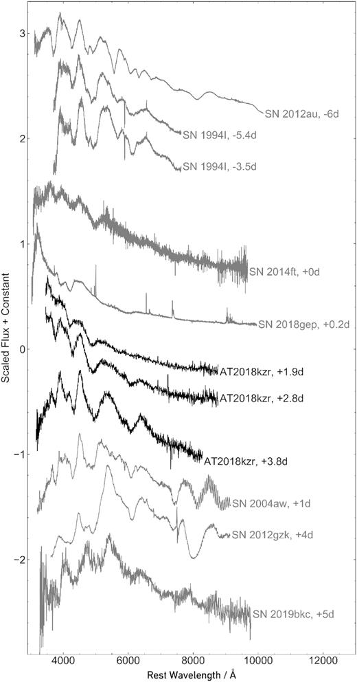
Photospheric spectra of AT2018kzr plotted alongside spectra of some fast-evolving Type Ic SNe. The spectra have features in common with AT2018kzr, helping to corroborate our line identifications. However, it is clear that the spectral shape of these other objects is redder than the early spectra of AT2018kzr. The names and phases of each SN are listed next to the spectra. The phases are relative to V-band maximum (SN 1994I; Yokoo et al. 1994), B-band maximum (SN 2004aw; Taubenberger et al. 2006), R-band maximum (SN 2012au; Takaki et al. 2013), r-band maximum (SN 2012gzk, SN 2014ft, SN 2018gep; Ben-Ami et al. 2012; De et al. 2018; Ho et al. 2019), g-band maximum (SN 2019bkc; Prentice et al. 2020), and discovery (AT2018kzr).
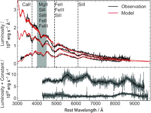
Observed spectra that were analysed in this work. Top panel: comparison of the three photospheric phase spectra (earliest at the top and latest at the bottom), which have been fully reduced and flux calibrated (black), with the corresponding models (red). Note that some regions of strong absorption by different ions have been annotated on the plot, to highlight what the dominant ion(s) are in our models at those wavelengths. Bottom panel: the two Keck spectra, taken at +7 d (upper spectrum) and +14 d (lower spectrum). These spectra have been rebinned to a dispersion of 10 Å pixel−1 (original in grey, and rebinned overplotted in black).
3 PHOTOSPHERIC PHASE SPECTRA
Our main aim was to produce a sequence of self-consistent models, with a uniform, one-zone composition, that consistently reproduce the first three spectra. To do this, we followed the abundance tomography technique (first presented by Stehle et al. 2005). We used tardis (Kerzendorf & Sim 2014; Kerzendorf et al. 2019), which is a one-dimensional Monte Carlo radiative transfer code for generating synthetic SN spectra. The code assumes that SNe have an opaque core, from which r-packets (analogous to bundles of photons) are radiated, with frequencies randomly assigned based on the characteristic blackbody temperature of an effective photosphere that is assumed to lie at the boundary of the opaque core. These r-packets propagate through the ejecta material, which is assumed to be in homologous expansion, and interact with the matter (either via scattering or absorption). The emergent packets are used to compute the synthetic spectrum.
Given how rapidly the transient evolved, we were not confident that any spectra taken at epochs later than the three NTT spectra could be meaningfully modelled with the assumption of an optically thick region and photosphere. tardis is only applicable when modelling SNe spectra in the photospheric phase, hence our decision to focus only on the three NTT spectra. We analyse the later spectra with an alternative method in Section 4. An initial attempt to model the +2.8 d spectrum was made by McBrien et al. (2019) to determine, approximately, the bulk composition of the ejecta. They determined that a composition dominated by O, Mg, and Si, along with a small amount of Fe, could reproduce the observed absorption features. In this paper, we go significantly further and calculate a detailed and consistent series of models to fit all of the early spectra.
There are three important observational parameters from the observed light curve of AT2018kzr (as presented by McBrien et al. 2019) that provide constraints for our spectral models. First, because the transient was so rapidly declining, the system had to have a low ejecta mass. McBrien et al. (2019) estimated an ejecta mass of Mej = 0.10 ± 0.05 M⊙, with which our spectral models should be compatible. Second, the constraints on the explosion epoch and the light-curve modelling fits predict an explosion epoch ∼1.7 d before first detection. Third, the bolometric luminosity of the transient is measured from the combined griz photometry.
Velocity ranges and density profile parameters for each of the models at the three different epochs. The density profile parameters and outer velocity boundary used for each epoch remained the same, while the inner velocity boundary shifted for each epoch.
| Time after | Minimum | Maximum | Density profile parameters | |||
|---|---|---|---|---|---|---|
| discovery (d) | velocity (|$\rm {km}\, s^{-1}$|) | velocity (|$\rm {km}\, s^{-1}$|) | v0 (|$\rm {km}\, s^{-1}$|) | t0 (d) | ρ0 (g cm−3) | Γ |
| +1.895 | 13 800 | 25 000 | 14 000 | 2 | 10−12 | 10 |
| +2.825 | 12 000 | 25 000 | 14 000 | 2 | 10−12 | 10 |
| +3.750 | 14 500 | 25 000 | 14 000 | 2 | 10−12 | 10 |
McBrien et al. (2019) predict the explosion epoch to be ≲3 d prior to first detection. However, we found that the spectra were fit best by using a model explosion epoch 4.6 d prior to first detection. We do not consider this result contradictory to that of McBrien et al. (2019), as they only weakly constrained the explosion epoch from the photometric light curve. The most recent non-detection was 2 d before first detection and was relatively shallow. Hence we could comfortably accommodate a slower rise time than that inferred by their bolometric light curve. Table 2 contains the time since explosion used for each of our best-fitting models.
tardis model parameters compared with those inferred from the photospheric light curve. Epoch refers to the estimated time from explosion from the light curve, whereas texp is that inferred from tardis. The Teff is not a free parameter; it is calculated consistently in tardis from the luminosity, velocity profile, and texp in each model.
| Epoch (d) | Model time since | Teff (K) | Luminosity from | Luminosity from LC | Luminosity from |
|---|---|---|---|---|---|
| explosion, texp (d) | tardis (erg s−1) | model (erg s−1) | photometry (erg s−1) | ||
| +1.895 | +6.5 | 13 200 | 1.30 × 1043 | 1.44 × 1043 | N/A |
| +2.825 | +7.5 | 12 100 | 9.22 × 1042 | 5.99 × 1042 | (8.4 ± 1.3) × 1042 |
| +3.750 | +8.5 | 8180 | 3.62 × 1042 | 2.64 × 1042 | (3.8 ± 0.9) × 1042 |
An important input parameter for tardis is the luminosity of the transient at each epoch. For this, we used the bolometric light-curve luminosities from McBrien et al. (2019), at the epochs of the NTT spectra. We were able to obtain good fits to the observed spectra without deviating more than ∼50 per cent from these luminosity values. The fact that we have managed to fit the spectra with similar values to those presented by McBrien et al. (2019) further corroborates their luminosity estimates for AT2018kzr. Table 2 contains the luminosities used in each of our tardis models. Also included are two different bolometric luminosities from McBrien et al. (2019). The first are the values determined from the measured data points. The second are the values of a physical model fit to the data. Both sets of data are included to highlight the variation between the photometric points and the best-fitting bolometric light curve, and to enable comparisons between the luminosity obtained from our tardis models, and the observed luminosity values.
In abundance tomography studies, it is expected that the inner ejecta velocity should either remain constant or decrease with time. This corresponds to the photosphere being either stationary or receding (see Stehle et al. 2005; Hachinger et al. 2009, for some examples). However in the case of AT2018kzr, our best-fitting models have an inner ejecta velocity that decreases from the first to second epoch, but then increases out from the second to third epoch. At face value, this would imply that the photosphere has moved outward. This may be possible in certain cases where, due to a change in density and temperature as the model evolves, the optical depth of the ejecta drastically increases. However, it is more likely that the photospheric approximation we are using is becoming more unreliable with time, and is introducing this feature into our models. Therefore, we emphasize that we do not interpret this as a physical property of the transient, and would advise the reader against drawing any strong conclusions from this aspect of the models.
Since the third photospheric spectrum was the most evolved, and contained the most features, we began by constraining the composition for this epoch first. We assumed a composition dominated by the most abundant intermediate-mass elements (IMEs: C, O, Mg, Si, and Ca) and iron-group elements (IGEs: Ti, Cr, Fe, Co, and Ni). Once a good fit for the +3.8 d spectrum had been obtained, the composition was kept constant, and the other parameters of the model were adapted to fit the earlier two spectra. Table 3 outlines the final composition we used to consistently fit the three NTT spectra. Also included are estimated uncertainties for the elemental mass fractions. These represent the upper and lower values that we could employ for the element without significantly altering the quality of the fit across any of our models (see Section 5.1 for further details of the O analysis in particular). Typically the uncertainties came from one of the three spectra that set the strongest constraints on an element (see Section 5.2). As shown in McBrien et al. (2019), the transient declined rapidly and in some phases the decline rate was similar to that of the one known kilonova, AT2017gfo. Hence we also attempted to model our spectra with a composition made from r-process elements, which would be plausible for a binary NS merger, and we discuss this in Section 3.4.
Elemental composition of our best-fitting model for the +1.9 d spectrum. The composition remains uniform for all epochs, apart from the effect radioactive 56Ni decay has on the composition. Also included are the limits we obtained for the maximum amounts of C and S that our best-fitting models could tolerate. These results help us to place an upper limit on the amount of the ejecta material that could be composed of these elements, which in turn can help us to constrain the progenitor system.
| Element | Relative mass fraction |
|---|---|
| C | <0.08 |
| O | 0.7|$^{+0.07}_{-0.15}$| |
| Mg | 0.13|$^{+0.10}_{-0.04}$| |
| Si | 0.09|$^{+0.03}_{-0.02}$| |
| S | <0.02 |
| Ca | (6|$^{+2}_{-1})\times 10^{-4}$| |
| Ti | (8 ± 0.8) × 10−4 |
| Cr | (5|$^{+4}_{-2})\times 10^{-4}$| |
| Ni | (2.5 ± 1) × 10−3 |
| Co | (3.5|$^{+3}_{-1})\times 10^{-3}$| |
| Fe | (3.5 ± 0.4) × 10−2 |
In Fig. 3, we plot the number fraction of the different ions for each of the elements included in the model. This illustrates how the number fraction of each ion varies in the ejecta material, for each of the three photospheric epochs. This comparison helps us to explain the spectral evolution of the models. As the transient evolves, it cools, and the elements present in the model become less ionized, resulting in lower ionization species appearing and/or becoming more pronounced in the later spectra.
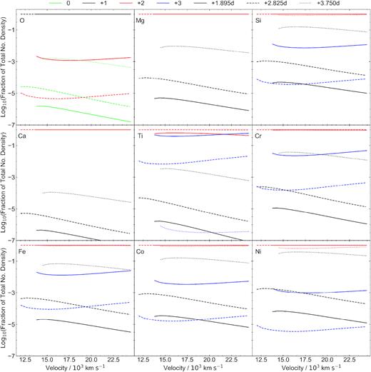
Ionization states of all elements included in the models across the three epochs. The solid lines correspond to the first epoch, dashed to the second epoch, and dotted to the third epoch. The lines are also colour coded to indicate how ionized the ejected material is (neutral to triply ionized).
3.1 Interpreting the +1.9 d spectrum
This spectrum has features in common with most of the Type Ic SN spectra plotted in Fig. 1, which suggests a composition broadly similar to that of Type Ic SNe, and this corroborates our line identifications. The spectral energy distribution (SED) of this spectrum is much bluer than most of these spectra (apart from that of SN 2018gep), suggesting that AT2018kzr is hotter than the other transients at the epochs plotted. The two prominent absorption features are more pronounced in this spectrum than the equivalent features in the spectra of SN 2018gep, SN 2014ft, and SN 2019bkc. These spectral differences hint that AT2018kzr is fundamentally different from these other transients, which we confirm from preliminary modelling of their spectra (e.g. we were able to satisfactorily fit the spectra of SN 2014ft with a relative mass fraction of Fe 10 times lower than that required for AT2018kzr).
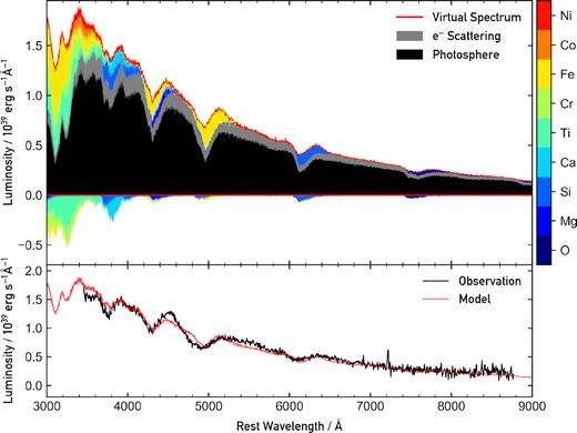
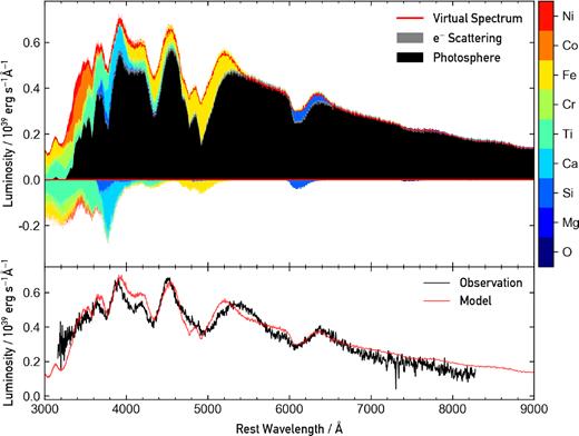
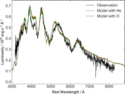
The bottom panel of Fig. 4 illustrates our best-fitting model plotted alongside the +1.9 d spectrum. The two prominent features in the observed spectrum are centred at ∼4200 and ∼4900 Å. Our model reproduces both of these features well. The upper panel of Fig. 4 highlights which elements contribute most to the absorption and emission features observed in the model spectrum. We define these plots as ‘Kromer’ plots (see fig. 6 in Kromer et al. 2013 for more information). From our Kromer plot, we can see that Fe is contributing the most to both of these features. The feature at ∼4200 Å is dominated by the Fe iii λλ4396, 4420, 4431 lines, with contribution from the Si iii λ4553 line. The feature at ∼4900 Å is dominated by the Fe iii λλ5127, 5156 lines. See Table 3 for the full composition used in the models.

Best-fitting model obtained for the +1.9 d spectrum obtained for AT2018kzr. Bottom panel: comparison of our best-fitting model to the observed spectrum. There is good agreement between the observed spectrum and our model, with all the absorption and emission features broadly agreeing. Top panel: associated Kromer plot for our model. The black region represents the contribution from the photosphere, and the grey represents the contribution from free electron scattering. The coloured regions correspond to the last physical interaction the escaping packets had; either absorption (region below zero) or emission (region above zero). This is a useful way to display which elements are contributing most to the various spectral features. At this epoch, the spectrum is dominated by Fe features (specifically Fe iii).
Beyond these two features, the rest of the spectrum is featureless. The important parameters of this tardis model are given in Tables 1 and 2, including time since explosion, effective photospheric temperature, and the inner luminosity. An important initial result from this spectrum is that it is unusually blue for the presence of strong Fe iii lines. The combination of the high temperature and strong Fe iii lines then requires a surprisingly high Fe abundance (see Table 3).
3.2 Interpreting the +2.8 d spectrum
This spectrum is almost as hot as the first epoch spectrum, and is still bluer than most of the Type Ic spectra in Fig. 1 (apart from SN 2018gep; comparable SED and hotter than SN 2014ft). The absorption features are also more pronounced in this spectrum than the corresponding features in the other hot, blue spectra. Our model implies these are now blends of Fe ii and Fe iii absorption, with contribution from Mg ii. Fe ii has previously been invoked to explain these broad absorption lines in Type Ic SNe (e.g. Hachinger et al. 2009). However, our spectrum is clearly much bluer and hotter than all the comparison Type Ic spectra in Fig. 1, and it is unusual, if not unprecedented, to observe such a hot continuum with strong Fe ii and Fe iii lines. From a purely empirical perspective, this suggests a larger Fe abundance, or higher density material (since a higher density equates to lower ionization states, and more Fe atoms), would be required to fit these lines in our models. We note that the possibility of high typical density in AT2018kzr at peak is potentially broadly consistent with the fast rise time of AT2018kzr compared to normal Type Ic SNe. Specifically, the fast rise is suggestive of a low ejecta mass (rise time to peak brightness, |$t_{\rm pk} \propto \sqrt{M_{\rm ej}}$|), and, since the density of ejecta material at peak, |$\rho _{\rm pk} \propto \frac{M_{\rm ej}}{t_{\rm pk}^3} \propto \frac{1}{t_{\rm pk}}$|, all other properties remaining equal (expansion velocity, opacity, etc.), the characteristic density of AT2018kzr would be higher than that of normal Type Ic ejecta material.
The bottom panel of Fig. 5 shows the best-fitting model plotted alongside the +2.8 d spectrum. The two features present in the previous spectrum (centred on ∼4200 and ∼4900 Å) are still prominent at this epoch. Two additional features have also appeared, one centred at ∼3700 Å, and the other centred at ∼6100 Å. We were able to successfully reproduce these two new features with our model, and we identify these features as Ca ii and Si ii, respectively.
Best-fitting model obtained for the +2.8 d spectrum. Bottom panel: there is good agreement between the observed spectrum and our model, with all the absorption and emission features broadly agreeing, with the exception of the emission feature at ∼4600 Å being underpronounced in our model. Top panel: associated Kromer plot for our model. The absorption and emission features due to different elements can be seen. At this epoch, the spectrum is again dominated by Fe, but with more pronounced features from the other elements included in the model, as compared with the model in Fig. 4.
The two absorption features that were present in the first spectrum are still reproduced by the tardis model. However, the features are no longer dominated by Fe iii; the feature at ∼4200 Å is produced by significant contributions from the Mg ii λλ4481.1, 4481.3 lines, Si ii λ4131 line, and Fe iii λλ4420, 4431 lines, while the feature at ∼4900 Å is produced by the Si ii λλ5041, 5056 lines, Fe ii λλ4924, 5018, 5169 lines, and Fe iii λλ5127, 5156 lines. The ejecta have cooled sufficiently between the first and second epochs to allow the Fe ii/Fe iii ratio to increase such that Fe ii now has a noticeable influence on the spectrum.
3.3 Interpreting the +3.8 d spectrum
This spectrum looks very similar to some of the Type Ic spectra in Fig. 1. At this epoch, AT2018kzr has cooled and become noticeably redder, matching the SED of the other spectra. Without the previous two spectra, the rapid spectral evolution of AT2018kzr would not be evident, and this spectrum could be mistaken as belonging to a fast Type Ic SN. However, these comparison objects do not exhibit the extremely rapid evolution we have observed for AT2018kzr. This hints at an alternative progenitor system that ejects material with a similar composition to that expected for Type Ic SNe.
The bottom panel of Fig. 6 compares this best-fitting model with the +3.8 d spectrum. The features in this spectrum are more prominent than in the previous two epochs, and are again satisfactorily reproduced by our model. The feature at ∼3800 Å is well reproduced by Ca ii, as before. The feature at ∼4200 Å is quantitatively reproduced by a blend of the Fe ii λλ4233, 4523, 4549, 4584 lines (similar to the previous epoch, but with negligible contribution from Fe iii, and less contribution from Mg ii). The feature at ∼4900 Å is produced by the Fe ii λλ4924, 5018, 5169, 5316 lines. Again, this is similar to the previous epoch, apart from the Fe iii. Finally, the feature at ∼6100 Å is modelled adequately by purely Si ii, as before. The model has now expanded and cooled sufficiently for the contributions of Fe iii to become negligible relative to Fe ii. In addition to the specific features we identify, there is significant line blanketing in the blue end of the observed spectrum below ∼3800 Å. In our model, we can replicate the strong absorption and reproduce the observed blanketing with a mix of IGEs (Ti, Cr, Ni, Co, and Fe).
Best-fitting model obtained for the +3.8 d spectrum obtained for AT2018kzr. Bottom panel: there is overall good agreement between the observed spectrum and our model, with all the absorption and emission features broadly agreeing. Top panel: associated Kromer plot for our model. The absorption and emission features due to the different elements can be seen. At this epoch, the spectrum has contributions from multiple elements at the same wavelength, leading to blended features. There are clearly significant contributions from all of the elements included in the model, especially at the blue end.
Our model slightly overestimates the flux towards the red end of the spectrum. Also, the absorption feature in the model at ∼4900 Å exhibits a double trough feature that is not present in the observed spectrum. There seems to be some discrepancy between our model and the observed spectrum in this region. Perhaps our model is missing an additional element/ion/transition that would blend these features. Alternatively, a change in velocity profile may blend these features into one. This may hint towards our model needing to have higher ejecta velocities, or a shallower density profile, allowing more material at higher ejecta velocities. Apart from this double trough feature, there is good agreement between the model and the observed spectrum, and so we do not place too much emphasis on this minor discrepancy.
3.4 Modelling the photospheric spectra with an r-process element composition
Given the fast declining nature of the light curve and rapid spectral evolution, we considered the possibility of AT2018kzr being a kilonova. McBrien et al. (2019) showed the light curve declined with a rate similar to AT2017gfo (with the light curve compiled from data from Andreoni et al. 2017; Arcavi et al. 2017; Chornock et al. 2017; Coulter et al. 2017; Cowperthwaite et al. 2017; Drout et al. 2017; Evans et al. 2017; Kasliwal et al. 2017; Smartt et al. 2017; Tanvir et al. 2017; Utsumi et al. 2017; Valenti et al. 2017). We note that although AT2018kzr was significantly more luminous, it has been hypothesized that additional luminosity can be produced in a NS–NS merger from a newly formed massive NS (see Metzger, Thompson & Quataert 2018). Therefore, the light-curve luminosity is not a sufficiently strong argument to rule out a kilonova. On this basis, we explored modelling the photospheric spectra with an alternative composition mixture that may be expected in binary NS mergers.
Kilonovae are expected to produce trans Fe-group and r-process elements, and so we generated models with the composition dominated by r-process elements from the first and second peaks (Kr–Ru and Te–Nd), to determine if the spectra of AT2018kzr exhibited any features due to these elements. We used the same explosion epoch as our previous models, presented in Table 2, while we gave ourselves freedom to vary the luminosity and ejecta velocity. The relative abundances used in the models were based on their relative mass fractions as observed in the photosphere of the Sun (from table 1 in Asplund et al. 2009) and we employed the atomic data from Kurucz & Bell (1995) for these elements. It is critical to note that the atomic line lists are incomplete for these heavy elements, and so our models will not truly represent the entire range of features that these elements would produce, but we follow this strategy as an exploratory exercise.
We were unable to produce a convincing fit with this composition and the parameters presented for our best-fitting models, for any of the three photospheric spectra. The model that came closest to reproducing the general spectral shape in any epoch was for the +2.8 d spectrum, and is shown in Fig. 7. Because of the incompleteness of the line lists, we cannot definitively state that the model’s inability to replicate observed features is proof that such a composition is ruled out. However, we can more convincingly determine that an r-process-dominated composition is implausible based on the features produced in our models that are clearly not in the observed spectrum (particularly the features around ∼4000 Å, which are dominated by Sr ii, Mo ii, Ru ii, and Ba ii).
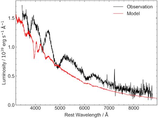
Comparison of one of our r-process model fits with the +2.8 d spectrum. None of the observed features are replicated by the model, and there are features in the model that are not present in the observed spectrum.
4 POST-PHOTOSPHERIC PHASE SPECTRA
In this section, we outline our analysis of the two Keck spectra (+7 and +14 d) shown in the bottom panel of Fig. 2. Since these appear to be either transitioning to, or are within, the nebular phase, the use of tardis for physical analysis is not justified. Therefore, we employed simple, alternative methods of analysis. The +7 d spectrum only has three discernible features, two of which have disappeared by the time the +14 d spectrum was obtained. The feature at ∼7800–9000 Å appears to have a P Cygni profile in the +7 d spectrum. If this is the case, then there is still scattering of radiation, and the material is optically thick for the wavelength of this line. By the time the +14 d spectrum was obtained, all trace of P Cygni absorption has disappeared, and is replaced with a pure emission feature. This implies that the region that created the P Cygni feature has become diffuse over time, and so the opacity for this line has dropped, preventing scattering. Since the two features cover the same wavelength range, we assumed they were produced by the same species, which we identified as the Ca ii triplet. The Ca ii triplet is commonly detected at late times in the spectra of many transients, and since the level that produces it has a low excitation energy, it can be easily excited. Additionally, it is excited from the ground state through the Ca H&K resonance lines, and so it is commonly observed with even a small Ca mass and composition. There are no other plausible transitions at this wavelength to produce this feature.
4.1 Interpreting the +7 d spectrum
We modelled the P Cygni profile of the Ca ii triplet using the generalized P Cygni calculation code developed by U. Noebauer.2 The code is based on a homologously expanding ejecta, as developed in the Elementary Supernova model (as detailed by Jeffery & Branch 1990). The program synthesizes a model P Cygni profile based on parameters specified by the user, which are the time since explosion, t, the optical depth of the line, τ, the rest wavelength of the line, λ0, two scaling velocities to infer the radial dependence of τ, ve, and vref, and the photospheric and maximum ejecta velocities, vphot and vmax, respectively. The photospheric velocity, or minimum ejecta velocity, is used to set the radius of the photosphere, which effectively sets the inner boundary for the model. In the context of the analysis we present here, we do not interpret this inner boundary as a true photosphere (which we would not expect to see at nebular phases). Instead we consider it as an approximate indication of the inner velocity boundary of the line-forming region for the Ca ii profile. Likewise, vmax provides a maximum velocity estimate for the line-forming region.
Since several of these parameters are unknown and need to be treated as free variables, we amended the code to make a parametrized search for the best model P Cygni profile to fit the data. The values were varied over a plausible range, and the best fit was determined based on χ2 statistics. The most physically interesting parameters are the minimum and maximum ejecta velocities, as well as the Sobolev optical depth, as these could be directly compared with those obtained from our tardis models, enabling us to better understand the evolution of the transient. Table 4 contains the parameters we obtained from our best-fitting P Cygni profile, which is shown in Fig. 8.
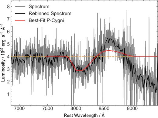
Model P Cygni profile compared with the observed +7 d spectrum. The orange dashed line marks the continuum.
Best-fitting model parameters for our analysis of the two late-time Keck spectra.
| Epoch (d) | Minimum ejecta | Maximum ejecta | Offset velocity, |
|---|---|---|---|
| velocity, vphot (|$\rm {km}\, s^{-1}$|) | velocity, vmax (|$\rm {km}\, s^{-1}$|) | voffset (|$\rm {km}\, s^{-1}$|) | |
| +7.056 | 20 000 | 26 000 | N/A |
| +14.136 | N/A | 23 700 | −2300 |
| Epoch (d) | Minimum ejecta | Maximum ejecta | Offset velocity, |
|---|---|---|---|
| velocity, vphot (|$\rm {km}\, s^{-1}$|) | velocity, vmax (|$\rm {km}\, s^{-1}$|) | voffset (|$\rm {km}\, s^{-1}$|) | |
| +7.056 | 20 000 | 26 000 | N/A |
| +14.136 | N/A | 23 700 | −2300 |
To obtain velocity estimates, we need to fit the absorption trough. In Fig. 8, it is clear that the P Cygni model profile matches the observed spectrum in this region. The model profile is unable to reproduce the emission region of the observed spectrum. This is a result of the feature not being produced purely by scattering; clearly the feature is in net emission, and as a result we underestimate the amount of flux in this region. However, this is not important, as we are only interested in obtaining velocity ranges for the line-forming region.
We obtained a minimum ejecta velocity, vphot ∼ 20 000 |$\rm {km}\, s^{-1}$|, and a maximum ejecta velocity, vmax ∼ 26 000 |$\rm {km}\, s^{-1}$|. These velocity values are, surprisingly, ∼2 times higher than those obtained from our tardis models. This is quite strong evidence that there is an additional high-velocity component of the ejecta that is not observed in the early, photospheric spectra. The computation for the P Cygni Ca ii line produces a velocity from the absorption trough that is fairly robust, as is the velocity estimates from our tardis models. Therefore, we believe the difference to be a real physical effect, and is an indication of additional high-velocity material, likely of low mass, which has been ejected beyond the emitting photospheric region (which is travelling at ∼12 000–14 500 |$\rm {km}\, s^{-1}$|).
We note that the level of the observed continuum to the red of the P Cygni peak falls significantly below that on the blue side. We attribute this to some oversubtraction of the host galaxy flux model as described in Appendix A, and do not attach any line forming significance to the discrepancy.
Our best-fitting model required a Sobolev optical depth, τ ∼ 1.3, which tells us that the P Cygni feature originates from a moderately optically thick region. Even though the +7 d spectrum appears to be nebular, the region forming the P Cygni feature is optically thick, at least for the wavelengths of the Ca ii triplet. The optical depth for these lines in all three of our tardis models is <1. Hence, the envelope is optically thin at these wavelengths in our tardis models. However, the optical depth in the tardis models becomes progressively larger with time. Since a P Cygni line requires an optically thick transition, we have a consistent picture of the Ca ii triplet line being optically thin at early epochs (probably due to high temperature), after which the material develops an optical depth around τ ∼ 1.3, providing the opacity for the absorption trough to form. We will see the next spectrum is consistent with the idea that the opacity in this line has dropped further, due to expansion, and a pure emission component has formed.
4.2 Interpreting the +14 d spectrum
In the +14 d spectrum, we observe the Ca ii feature to be purely in emission. We fit a Gaussian profile to the emission feature, to further estimate the velocity of the ejecta material. By assuming the feature is solely produced by the three transitions of the Ca ii triplet, we can estimate the ejecta velocity, and the velocity offset, i.e. the velocity we observe the material to be travelling towards or away from us, relative to the bulk motion of the rest of the expanding material. We began by generating three individual Gaussians centred on the rest wavelengths of the three Ca ii triplet lines, and assigned each of them the same width and a height that was representative of their relative strengths (if we assume the material is optically thin). We then sum these and fit the observed feature with this combined Gaussian. Fig. 9 shows the corresponding best-fitting composite Gaussian obtained.
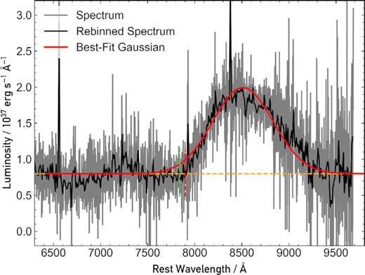
Comparison of our best-fitting Gaussian to the observed emission feature in the +14 d spectrum. The grey line represents the original spectrum, and the black line overplotted represents the same spectrum but rebinned to a dispersion of 10 Å pixel−1. The red line represents our best-fitting Gaussian. The horizontal orange dashed line corresponds to where we estimated the continuum of the spectrum to lie. The small vertical red dashed line at the blue end of the emission feature corresponds to where we estimate the blue wing of the feature has blended into the continuum. From this point, we can estimate the maximum velocity of the ejecta producing this feature. The vertical dashed green line represents where the blue wing blended into the continuum in the +7 d spectrum, determined by our P Cygni fit.
From this simple model, we estimate where the emission feature blends into the continuum. This point is on the blue wing of the emission feature at ∼7900 Å (marked by a small vertical dashed red line in Fig. 9). From this, we obtain a maximum ejecta velocity, vej ∼ 23 700 |$\rm {km}\, s^{-1}$|, and an offset velocity (blueshift) voffset ∼ −2300 |$\rm {km}\, s^{-1}$|. The offset velocity is with respect to the rest wavelength of the combined feature, i.e. we have to shift each of the three components by −2300 |$\rm {km}\, s^{-1}$| to match the peak of the observed feature.
The maximum velocity from the emission line is similar to the maximum velocity implied by the absorption trough of the P Cygni profile in the +7 d spectrum. This is consistent with both features being from the same high-velocity material, which has gone from a Sobolev optical depth of τ ∼ 1.3 to optically thin between the two epochs. Hence, we have consistent evidence of a high-velocity component of the ejecta that is producing this observed feature, but is not contributing to the spectra at earlier epochs. Our offset velocity indicates that there is perhaps some inhomogeneity in the ejecta material, where we see excess material travelling with a component in our line of sight. This offset velocity is only a small fraction of the maximum observed ejecta velocity (∼9.7 per cent) and so is likely not an issue with our interpretation of the emission feature being produced by the Ca ii triplet.
Similar blueshifted Ca ii lines in the nebular phase of other fast-fading transients have been found previously, perhaps indicating a similar physical cause. Two examples include SN 2012hn (Valenti et al. 2014) and SN 2005E (Perets et al. 2010; Waldman et al. 2011). Foley (2015) studied 13 of these Ca-rich objects, and as part of their work, determined the velocity offsets for the [Ca ii] λλ7291, 7324 lines. They found that three of their sample (SN 2003dg, SN 2005cz, and SN 2012hn) had offset velocities >−1000 |$\rm {km}\, s^{-1}$|, with SN 2012hn exhibiting the largest offset velocity, at −1730 |$\rm {km}\, s^{-1}$|. The offset velocity we obtain for our Ca ii triplet feature (∼−2300 |$\rm {km}\, s^{-1}$|) is larger than previous Ca-rich objects, by ∼33 per cent. An even larger offset velocity has been observed for SN 2019bkc (Chen et al. 2020; Prentice et al. 2020), which exhibits an offset velocity of ∼−10 000 |$\rm {km}\, s^{-1}$|, for the Ca H&K lines, the [Ca ii] λλ7291, 7324 lines, and the Ca ii triplet.
5 DISCUSSION AND INTERPRETIVE ANALYSIS
5.1 Oxygen as the dominant element
The dominant element, by mass fraction, in all of the models is O, which makes up ∼70 per cent of our ejecta material. However, the Kromer plots for all three models exhibit no significant emission or absorption features due to any ion of O. The emitting region is too cool to produce the optical O ii lines seen in many hot, blue superluminous SNe (these may even require non-thermal excitation; Mazzali et al. 2016), and too hot for O i lines to form. This would hint that we have no need for it in the model. However, if we remove O and drop the total amount of material in the ejecta by ∼70 per cent, the spectrum appears significantly different. This is due to there being many fewer free electrons in the ejecta material when O is removed, as O is effectively acting as an inert electron donor. Much of the O is ionized and provides free electrons for electron scattering processes in the spectrum, without producing specific O features (which are not observed). Additionally, if everything else remains equal, a higher free electron density will lead to lower ionization states in the model. To demonstrate that free electron donation is occurring, we calculated models with an alternative filler element, i.e. one that donates free electrons, but also is not likely to produce spectral lines in the optical regime. We chose He, but could have also used C, Ne, or some mixture of the three, as these are all elements that are predicted and/or observed in significant quantities in different SN systems.
We varied the total amount of material above the photosphere, and varied the ratio of the filler element relative to the other elements. We imposed the restriction of maintaining the mass fraction ratio of the elements that contribute to the spectral features. These ratios were taken from our best-fitting models (see Table 3). We were able to obtain a good model for the +3.8 d spectrum with He as our filler element, as demonstrated in Fig. 10. While we cannot rule out a significant amount of He being present, we propose that O is more likely and a physically motivated choice due to the significant fraction of IMEs in the ejecta that are required to model the observed features (see Höflich, Wheeler & Thielemann 1998; Seitenzahl et al. 2013).
Comparison of the +3.8 d spectrum with the best-fitting model previously presented in Fig. 6, and the new best-fitting model, with He as the filler element instead of O. It is clearly evident that the fits almost perfectly agree with each other, and the observed spectrum.
5.2 Limits on carbon, sodium, and sulphur
To further constrain the composition, we estimated upper limits on three elements (C, Na, and S) that have no visible lines in any of the spectra. C and S are produced by the α-process, while Na is synthesized via carbon burning. They are of high abundance in Solar system ratios and are commonly produced in various core-collapse and thermonuclear explosion scenarios. Hence it is of interest to determine if their lack of observed lines can place an upper limit on their mass fraction in the ejecta.
For these tests we reverted to the best-fitting models that used O as the filler. We replaced various mass fractions of O with the same mass fraction of the element we were considering, i.e. to calculate a model with C mass fraction of 2 per cent, we removed 2 per cent of the total mass fraction from O, and kept all the other elements equally abundant. The bottom spectrum in Fig. 11 illustrates the effect that adding in a 2 per cent mass fraction of S has on our best-fitting model. We clearly do not observe the S feature at the model wavelength (5200–5600 Å) in the observed spectrum, which we attribute to the ‘w’ S ii feature at 5640 Å, and so this sets a robust constraint on the mass fraction of S that can be present. We found that we could also constrain the amount of C to <8 per cent (see the top spectrum in Fig. 11). There are three C features present in the model, at ∼4600, ∼6400, and ∼7000 Å, due to the C ii λλ4745, 6580 and 7234 lines. The amount of Na in the spectrum was harder to constrain as our best-fitting models at all three epochs could accommodate a large mass fraction of Na without producing strong features. The middle spectrum in Fig. 11 shows the effect of adding 40 per cent Na to the spectrum. The only noticeable effect is a weak feature at 5700 Å, which we attribute to the Na i D λλ5890, 5896 lines. Table 3 contains the upper mass limits we obtained for C and S in our three models. Na is not included as it was very unconstrained for all of our models.
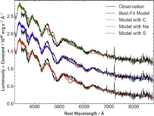
Comparison between the +2.8 d spectrum, our associated best-fitting model, and three models identical to our best fit, but with 8 per cent of the O mass fraction replaced with C (top), 40 per cent replaced with Na (middle), and 2 per cent replaced with S (bottom).
6 DISCUSSION OF PROGENITOR SYSTEMS
Given the constraints on the chemical composition of the ejecta, we now discuss the four progenitor systems and explosion mechanisms that we consider to be most viable for AT2018kzr. Three of these were previously summarized by McBrien et al. (2019): an ultrastripped core-collapse SN, accretion-induced collapse (AIC) of a WD, and a WD–NS merger (or WD–BH merger). We also include discussion on a fourth explosion mechanism: explosion of a double WD merger remnant. We begin by noting that some systematic uncertainties arise from both our spectroscopic modelling, and the light-curve modelling performed by McBrien et al. (2019). tardis has some intrinsic uncertainty for estimates of the ionization and excitation levels for all elements in the model. This may introduce systematic uncertainties in the determined composition. The light-curve modelling of McBrien et al. (2019) is based upon a simple approximation for homologously expanding material, with constant opacity. The fairly simple physics employed is likely to result in a systematic uncertainty in the ejecta mass. Accordingly, we suggest that all specific values extracted from the modelling should be treated with some leeway (in the following we will adopt a factor of ∼2 as indicative of such limitations).
The results from Sections 3–5 can be summarized as follows. We require a significant mass fraction of Fe to fit the three photospheric spectra consistently (3.5 ± 0.4 per cent), and a well-constrained (but much smaller) mass fraction of Ni and Co of 0.25 ± 0.1 per cent and |$0.35^{+0.3}_{-0.1}$| per cent, respectively (see Table 3). The high mass fraction of Fe is unusual but appears a robust conclusion. The three early spectra are both blue and hot and simultaneously have strong absorption features due to Fe ii and Fe iii. It is unusual, if not unprecedented, to find this combination since at Teff ∼ 13 000 K, these ions produce relatively weak photospheric features (for compositions with solar Fe ratios). Any explosion scenario must explain this very high Fe/(Ni+Co) ratio. It is normally assumed that most, if not all, Fe that is observed in SNe and transients is 56Fe from the decay chain of 56Ni and 56Co (or pre-existing, as in Type IIP SNe). However, if the epoch of our first model is 6.5 d after explosion, then 47.6 per cent of any explosively formed 56Ni would still persist, with 50.7 per cent converted to 56Co, and only ∼1.7 per cent could have decayed to stable 56Fe. The mass fractions imposed by our models limit the amount of Ni and Co to ∼10 per cent of the mass fraction of Fe. Hence our measured composition is highly discrepant, by a factor of ∼300, with the expected ratios of Ni, Co, and Fe if they were synthesized from explosively produced 56Ni.
Furthermore, our model for the +1.9 d spectrum requires 1.39 × 10⁻² M⊙ of ejecta material (above the opaque core) to form the synthetic spectrum, and 3.5 per cent of this is made up of Fe (4.85 × 10⁻⁴ M⊙). If we assume all the Fe in our first model is 56Fe produced by radioactive 56Ni decay, and we also trust our model explosion epoch, then we would need an initial 56Ni mass of 2.89 × 10⁻² M⊙. This is larger than the total mass of material required to form the spectrum, and hence is an unphysical solution. We conclude that the spectrum must be intrinsically Fe-rich, and that this Fe must be another stable isotope, plausibly 54Fe.
In Table 5, we summarize the pros and cons of each progenitor system in the context of the observational constraints we now have for AT2018kzr, and we discuss these in detail in the next four subsections.
Summary of the pros and cons of each of the progenitor systems considered for AT2018kzr.
| Ultrastripped | Accretion-induced | Double WD | Merger of a WD | |
|---|---|---|---|---|
| core-collapse SN | collapse of an ONe WD | merger systems | with an NS/BH | |
| Peak brightness | Bad | Possiblea | Good | Possibleb |
| Light-curve evolution | Bad | Possiblec | Good | Good |
| Velocity of ejecta | Good | Bad | Good | Goodd |
| Ejecta mass | Good | Good | Good | Possiblee |
| Bulk composition | Good | Bad | Bad | Good |
| Fe/Ni ratio | Bad | Bad | Bad | Good |
aCapable of producing a magnetar, which can power the light curve.
bCapable of reaching the observed luminosity of AT2018kzr, with the help of high-velocity winds launched off the disc.
cLight-curve evolution too fast in the models discussed, but a higher ejecta mass would act to extend the light curve.
dThe bulk velocity of the ejecta material agrees with our photospheric estimates for ejecta velocity.
eThe ejecta mass obtained from light-curve modelling is lower than that estimated from the models discussed, but these values are dependent on the specific merger, which make it difficult to get good approximations.
6.1 Ultrastripped core-collapse supernova
Tauris, Langer & Podsiadlowski (2015) define an ultrastripped SN as an exploding star that has been stripped by a degenerate companion (the amount of stripping is expected to be more than is possible by a non-degenerate companion). Typically, ultrastripped SNe have pre-explosion envelope masses of ≲0.2 M⊙, but in some cases can have envelopes as low as ∼0.008 M⊙. Explosions of these objects will have correspondingly small ejecta masses, and therefore fast rise times, compared with normal core-collapse light curves. In particular, they are predicted to be fast-evolving, and fainter than typical Type Ibc SNe. Tauris et al. (2015) have no spectroscopic predictions for ultrastripped SNe, but the ejecta composition are expected to be broadly similar to that of Type Ibc SNe, as they arise from similar progenitor systems.
Moriya et al. (2017) present the nucleosynthetic yields they obtain for their ultrastripped core-collapse model, which was based on the ultrastripped progenitor presented in Tauris et al. (2013). They evolve a star from the He zero-age main sequence (ZAMS), with the mass-loss rates expected from binary interaction (Roche lobe overflow). This results in a 1.5 M⊙ stripped He star, with a CO core of 1.45 M⊙. This progenitor was then evolved until it collapsed, and the ejecta properties were determined for different ejecta energies and masses. The composition predicted by their models broadly agree with our composition, except for the 56Ni production (they predict a range of 56Ni abundances for the different models, with fractions between 0.13 and 0.20 of the total ejecta). Also, the light curves decline much too slowly to replicate the behaviour of AT2018kzr.
Hachinger et al. (2012) present a model composition for SN 1994I, a well observed, low-mass, stripped-envelope Type Ic SN (e.g. see their fig. 7). They derive a composition for SN 1994I empirically, and so we compare their results to ours, since we have adopted a similar approach. Additionally, the comparison to a Type Ic SN is useful as our spectra have some similarities with the spectra of Type Ic SNe (see Fig. 1). The main difference between our method to derive the composition for AT2018kzr and those of Hachinger et al. (2012) is that we have used a uniform, one-zone model, whereas they have a layered structure for their ejecta. Aside from this, our composition looks strikingly similar for the IMEs. In particular, their composition in the 9500–13 500 |$\rm {km}\, s^{-1}$| velocity range appears almost identical to ours, with the mass dominated by O. There is ∼5 per cent C, and ∼few per cent Na, both of which are permitted by our model. In this region, they infer significantly more Ni and less Fe than we have in our models. To summarize, if we had a Type Ic SN with the composition Hachinger et al. (2012) determine for SN 1994I, but with the outer layers stripped off (>13 500 |$\rm {km}\, s^{-1}$|), and the photosphere located at 9500 |$\rm {km}\, s^{-1}$|, then our envelope composition would generally match the IMEs.
The light curves of Type Ic (and also ultrastripped core-collapse) SNe are thought to be powered by radioactive 56Ni decay. The inclusion of Ni in spectrophotometric models of Type Ic explosions is mainly for this reason, as well as to provide a mechanism to produce Fe, which contributes significantly to the photospheric and nebular spectra. As shown by McBrien et al. (2019), the light curve of AT2018kzr is not compatible with 56Ni powering.
As discussed above, we conclude that the Fe required to form the strong absorption lines is unlikely to be 56Fe and must be another stable isotope (54Fe). Such ratios of Fe isotopes and Fe/(Ni+Co) ratios are not predicted in any core-collapse mechanism and hence this makes the ultrastripped SN scenario unlikely. The fact that McBrien et al. (2019) found that a central powering mechanism is required to produce the observed luminosity also disfavours the ultrastripped progenitor in a binary system. Any process that severely removes mass will also serve to decrease the angular momentum, making a rapidly rotating NS remnant unlikely (Müller et al. 2018).
6.2 Accretion-induced collapse of an ONe white dwarf
Accretion-induced collapse (AIC) may occur when an ONe WD accretes material from its companion object and grows close to the Chandrasekhar mass, causing it to reach central densities that trigger electron capture (see Brooks et al. 2017a for a more in depth description). At this point, it is expected that the WD collapses. When these objects collapse, they are thought to eject very little material (|${\lesssim} 10^{-2}\, \mbox{M$_{\odot }$}$|), as most of the material will collapse into an NS. The amount of ejected material and its properties are dependent on the properties of the WD progenitor.
Darbha et al. (2010) perform light-curve and spectroscopic analysis of AIC models. Specifically, they modelled the accretion disc that is predicted to form around the newly formed NS. For their analysis, they considered two different ejecta masses (|$10^{-2}$| and |$3\times 10^{-3}\, \mbox{M$_{\odot }$}$|), with three different ranges of electron fraction (|$Y_{\rm e}$|) considered for each of these masses (0.425–0.55, 0.45–0.55, and 0.5–0.55). These models have less ejected material than AT2018kzr (see McBrien et al. 2019, where they conclude the ejecta mass to be |${\sim} 0.10\pm 0.05\, \mbox{M$_{\odot }$}$|). However, the findings of Darbha et al. (2010) are still useful to compare to our results.
First, they predict that the outflow material will have very high velocity (∼0.1c), which is significantly higher than the values we determine from our modelling of the early photospheric phase spectra. Second, a defining characteristic of AIC is that the disc will process material via nuclear statistical equilibrium (NSE), meaning little to no IMEs will be synthesized. This contradicts our model results, which show that we only need ∼few per cent IGEs, with the rest of the ejecta dominated by IMEs. The ejecta material for the models in Darbha et al. (2010) is dominated by Ni, which we do not observe in the spectra of AT2018kzr. Additionally, the evolution time-scales for the models presented by Darbha et al. (2010) are faster than that of AT2018kzr, although our larger ejecta mass may help reconcile this, since more ejected material tends to favour slower rise times. The model light curves are also much dimmer than that observed for AT2018kzr.
The results presented by Darbha et al. (2010) broadly agree with the predictions made by Metzger, Piro & Quataert (2009). In this work, Metzger et al. (2009) conclude that the ejecta material from AIC will typically have velocities, vej ∼ 0.1–0.2c, and will be predominantly made up of Ni. The multidimensional simulations of AIC in WDs of Dessart et al. (2006) suggest a very modest ejecta mass of ∼10−3 M⊙, with about 25 per cent of that being 56Ni. Such an ejecta mass and composition is not compatible with the observed light curve nor with the composition we derive here.
The work of Dessart et al. (2007) shows that a magnetar may be produced in certain AIC systems, which is capable of powering the light curve of AT2018kzr (as shown by McBrien et al. 2019). They predict that these systems would eject significantly more material (∼0.1 M⊙) than systems that do not produce a magnetar. They also predict negligible Ni production. However, they expect the ejected material to have an electron fraction, Ye ∼ 0.1–0.2, leading them to suggest that the ejecta of an AIC with a magnetar will be dominated by r-process elements, which does not agree with the composition we obtained from our spectral modelling.
6.3 Double white dwarf merger systems
Brooks et al. (2017b) present observational predictions for fast and luminous transients that arise from the explosion of long-lived WD merger remnants. In this scenario, a He WD merges with a more massive CO or ONe WD. Most of the mass of the He WD forms an extended envelope around the massive WD, which burns for ∼105 yr. The massive WD accretes material from this extended envelope, and as it approaches Chandrasekhar’s mass, it may undergo electron capture, and collapse to an NS. The energy released by this collapse is injected into the extended envelope surrounding the NS. The models presented by Brooks et al. (2017b) have luminosities of ∼2–3 × 1043 erg s−1 1 d after explosion. This agrees well with our observations for AT2018kzr (Lpeak ∼ 2 × 1043 erg s−1). Their light curves are short-lived, which again agrees with our observations of AT2018kzr.
There is some variation in the photospheric velocities of the models in Brooks et al. (2017b), but all models have photospheric v ∼ 15 000 |$\rm {km}\, s^{-1}$| at 2/3 d, dropping to ∼10 000 |$\rm {km}\, s^{-1}$| after 5/6 d. These velocities agree well with those obtained from our spectroscopic modelling of the photospheric spectra of AT2018kzr. The models presented have ejecta masses of 0.1 and 0.2 M⊙, which is what we expect for AT2018kzr (from light-curve modelling; see McBrien et al. 2019). However, the ejecta composition does not match what we obtain from our spectroscopic modelling. Brooks et al. (2017b) predict an ejecta dominated by Mg and C (60/65 per cent Mg, 31/27 per cent C for envelope masses, |$M_{\rm env} = 0.1/0.2 \, \mbox{M$_{\odot }$}$|). Our models cannot accommodate this amount of C and Mg. Their models also predict much less Si (1.5/1.4 per cent) than we require for our models (9|$^{+3}_{-2}$| per cent). There are no abundances quoted for IGEs, and so we cannot comment on their abundance. This progenitor system is disfavoured based on the discrepancy between the predicted composition, and the composition we have derived for AT2018kzr from our spectral modelling.
6.4 Merger of a white dwarf with a neutron star or black hole
A WD–NS merger results from a binary system, in which a WD and an NS inspiral as the system radiates energy in the form of gravitational waves. Eventually the orbit shrinks to the point where the WD is disrupted, and a disc of WD material is formed around the NS. According to theoretical models, the temperature and pressure in the disc facilitates nuclear burning, enabling elements up to the Fe-peak to be synthesized. A WD–BH merger forms in exactly the same way, but with a stellar mass BH instead of an NS. A number of different simulations of such mergers have been performed (Metzger 2012; Margalit & Metzger 2016; Fernández et al. 2019; Zenati et al. 2020), with quantitative predictions for nucleosynthesis, ejecta mass, chemical composition, and velocity structure. In the following, we will summarize the results and conclusions of these theoretical works, and compare our results to the predictions made.
6.4.1 Margalit & Metzger (2016)
The model CO WD–NS mergers of Margalit & Metzger (2016) show compositions dominated by unburnt C and O, which are located in the outer region of the disc, with less abundant, heavier elements (relative to C and O) located in the inner regions of the disc, as this is where they are synthesized. The heavier elements originate at smaller disc radii, where the outflow velocity is large, and so are ejected at higher velocity compared with the unburnt C and O that is expelled. The outflow of material from wind loss is expected to contain a significant fraction of C, but we have a strict upper limit of <8 per cent C from our spectral models. We suggest that the lack of C in AT2018kzr can be explained by the disrupted star being an ONe WD rather than a CO WD. Our spectral synthesis requires significantly more Mg than is synthesized in these CO WD–NS mergers. All the Mg ejected in the Margalit & Metzger (2016) models is synthesized in the disc. However, ONe WDs can have small quantities of Mg in their cores (|${\lesssim} 0.05\, \mbox{M$_{\odot }$}$|; Takahashi, Yoshida & Umeda 2013), which may help to reconcile the discrepancy between our Mg abundance, and that in the CO WD–NS mergers presented by Margalit & Metzger (2016).
The amount of 54Fe synthesized in the CO_fid model presented by Margalit & Metzger (2016) makes up ∼1.1 per cent of the total ejecta at the simulation end time and the amount of 56Ni synthesized is ∼6 times less (∼0.19 per cent). Our tardis model for AT2018kzr requires 14 times more Fe than Ni, which is a factor of ∼2 more than in the CO_fid model of Margalit & Metzger (2016). The range of CO WD mergers of Margalit & Metzger (2016) have ratios 1.5 ≲ 54Fe/56Ni ≲ 7.5, with most models producing ratios at the higher end. While our inferred ratio is higher, it is still is in good qualitative agreement with the Margalit & Metzger (2016) calculations. It is unusual to have more 54Fe than 56Ni, and so the fact that these models by Margalit & Metzger (2016) are in this regime is compelling.
The outflow velocity of the ejecta in these models spans a wide range. The unburnt C and O can have velocities as small as ∼2000 |$\rm {km}\, s^{-1}$|, while the heavier elements possess higher velocities. The heavier elements (elements produced from oxygen and silicon-burning) originate from smaller radii in the disc, since higher temperatures are required for them to be synthesized. The mass weighted outflow velocity for the CO_fid model, <vw> ∼ 12 000 |$\rm {km}\, s^{-1}$|, which agrees well with the velocities from our spectroscopic modelling. We do not have evidence of significantly higher velocity material in the early photospheric spectra. However, a smaller amount (by mass) of high-velocity ejecta from the inner region of the disc may explain the high-velocity Ca ii feature we observe in the two later, post-photospheric spectra (see Section 4). This second component is moving at velocities between 20 000 and 26 000 |$\rm {km}\, s^{-1}$|, with a moderate asymmetry detected through the blueshift of the emission feature (∼2300 |$\rm {km}\, s^{-1}$|).
The luminosity of this model CO WD–NS transient would reach a peak luminosity, Lpeak ∼ few 1040 erg s−1 if it were powered solely by 56Ni decay. This is significantly lower than that of AT2018kzr. Margalit & Metzger (2016) proposed that the luminosity of the transient can be significantly enhanced by high-velocity winds, which are launched off the disc at late times. These winds collide with the bulk of the ejecta released earlier, thermalizing some fraction of the wind’s kinetic energy. This is quite an efficient heating process and has the capability of boosting the luminosity to ≲2 × 1043 erg s−1 (for only 10 per cent thermalization efficiency). Margalit & Metzger (2016) also predict that the NS may be spun up to a period, P ∼ 10 ms. If it has a large magnetic field (B ≳ 1014 G), the resultant energy deposition from magnetar spin-down could also power the light curve (see McBrien et al. 2019 for a semi-analytic model of magnetar powering). The rise time for the models in Margalit & Metzger (2016) agree with the explosion epoch we obtain from our spectroscopic modelling. The total amount of material ejected from their CO WD–NS models is ∼0.3 M⊙, which is somewhat larger than the mass inferred from the light-curve modelling presented by McBrien et al. (2019). However, within the systematic uncertainties of both approaches (which are not 3D, hydrodynamic models) a difference of a factor of ≲2 is not a significant discrepancy.
6.4.2 Metzger (2012)
Metzger (2012) presented earlier models for a wider range of merger scenarios, including CO WD–NS, He WD–NS, CO WD–BH, and ONe WD–BH mergers. In each case the mass of the compact remnant was NS = 1.4 M⊙ and BH = 3 M⊙. The ejecta velocities for the heavy elements synthesized in the inner regions of the disc are predicted to be largest for the ONe WD–BH system, with mean disc wind velocities, |$\bar{v}_{\rm w} \gtrsim 3\times 10^{4}$| |$\rm {km}\, s^{-1}$|. However, it is predicted that most of the ejected material will reside in a single shell of material at large radii, with much lower expansion velocity. The fast ejecta originating from the inner regions of the disc are then expected to collide with this slow moving ejecta, and deposit the majority of its energy in this shell, causing it all to achieve a mean velocity, |$\bar{v}_{\rm ej} \sim 10^{4}$| |$\rm {km}\, s^{-1}$|. The amount of ejected material for the models range from ∼0.3 to 1.0 M⊙, which is higher than that permitted by the AT2018kzr light curve (McBrien et al. 2019). However as noted above, the lower end of that range is compatible, given the simplicity of each of the models.
Metzger (2012) presented two ONe WD–BH merger models and both produced significant 54Fe mass fractions of 12 and 22 per cent and 56Ni mass fractions of 5.4 and 1 per cent. The high mass fraction of 54Fe is qualitatively similar to our finding, but the 56Ni mass predicted is significantly higher than our spectral constraints. We obtain a ratio of 54Fe/56Ni ∼ 14 from our spectroscopic modelling, which falls between the values of 2.2 and 22 of the Metzger (2012) models. If the accretion rate by the BH was higher, it would perhaps decrease the Fe and Ni ejected (as these originate from the innermost parts of the disc), bringing their mass fractions more in line with our predictions. Additionally, if the accretion rate was higher, the total amount of ejected material would also decrease. We note that significant He is predicted (15 and 13 per cent) in these ONe WD–BH mergers, and we can accommodate He as a filler, or partial filler, element (see Section 5.1). The models by Metzger (2012) also produce significant amounts of Si (17–18 per cent) and S (7–8 per cent) that are factors of ∼2 and ∼4 higher than inferred from the spectra of AT2018kzr.
6.4.3 Fernández et al. (2019)
Fernández et al. (2019) present more recent and detailed models for ONe WD–BH mergers, with the mass of the BH = 5 M⊙. They evolve three models for an ONe WD–BH merger: two for a non-rotating BH and the third model with a rotating BH (with a dimensionless spin of χ = 0.8), with different inner boundaries. The maximum velocity of the ejecta material for the non-rotating, large-boundary model is ∼1.5 × 10⁴ |$\rm {km}\, s^{-1}$|, while for the non-rotating, small-boundary model, this increases by a factor of ∼2. The material ejected should be dominated by unburnt WD material, with 24, 34, and 43 per cent composed of burning products. The rise times of these transients are predicted to be on the order ∼few days, with peak luminosity ∼1040–1041 erg s−1. This luminosity can be boosted by circumstellar interaction or late-time accretion on to the central object. For example, Fernández et al. (2019) point out that accretion powering (as in Dexter & Kasen 2013) could boost the model luminosity, L ∼ 1043 erg s−1, within a time to peak of t ∼ 3 d, rather similar to AT2018kzr. The predicted ejecta mass for the ONe WD–BH models is only quoted for the model with the large inner boundary (Mej = 0.72 M⊙), which is much larger than permitted by the light-curve model for AT2018kzr (see McBrien et al. 2019). It is worth noting that the models of Fernández et al. (2019) synthesize less Fe than the models presented by Metzger (2012) and Margalit & Metzger (2016), and do not predict a larger abundance of Fe than Ni. The amount of Mg synthesized in the three models is 5, 5, and 3 per cent, which is lower than the amount we require for our models (13|$^{+10}_{-4}$| per cent). One of their models also overproduces Si relative to our estimate for AT2018kzr. They produce 11, 16, and 11 per cent in their three models, whereas we require 9|$^{+3}_{-2}$| per cent for our models. Hence the velocity, composition, and plausible luminosity of an accretion-powered transient all broadly agree with what we infer for AT2018kzr, with some discrepancies as described.
6.4.4 Zenati et al. (2020)
Not all work on modelling WD–NS mergers predicts observational properties similar to what we have observed for AT2018kzr. For example, Zenati et al. (2020) predict that the light curves of these mergers will be faint and red. They present models for a range of WD–NS mergers. Their models include both He and CO WDs, with masses of 0.55, 0.63, and 0.8 M⊙, and NS masses of 1.4 and 2.0 M⊙. The bolometric luminosities are expected to reach ≤−15, which is lower than that observed for AT2018kzr. The models presented have rise times of ≤10 d, which is broadly consistent with the rise time of AT2018kzr. The mass of unbound material at the end of the simulations span the range 8 × 10⁻³–0.2 M⊙. The upper end of this range agrees well with the amount of material needed to power the light curve of AT2018kzr. The models by Zenati et al. (2020) do not predict that more Fe will be synthesized than Ni, which we require for our models. However, these nuclear yields were obtained from their 3D calculations, which vary significantly from previous calculations performed in 2D. The overall SED of the models in Zenati et al. (2020) do not match that of AT2018kzr, but many of the other predicted properties broadly agree.
7 CONCLUSIONS
In this work, we have presented spectroscopic analysis of the extraordinarily fast-evolving transient, AT2018kzr. We obtained a convincing sequence of self-consistent models that replicate the early observed photospheric spectra. From these models, we extracted properties of the ejecta, such as the velocity and composition (see Tables 1 and 3). The models also provided us with luminosity estimates for the transient, and an explosion epoch. The ejecta is primarily composed of the intermediate-mass elements O, Mg, and Si (70, 13, and 9 per cent, respectively) and we set a restrictive limit on the amount of C (≤8 per cent). Most importantly we find that a large mass fraction of Fe is required to explain the strong absorption features in the observed spectra (3.5 per cent), which are predominantly formed by Fe ii and Fe iii. In addition, low Ni and Co mass fractions are required (0.25 and 0.35 per cent, respectively). The most common stable Fe isotope, 56Fe, is formed through the decay of 56Ni→56Co (half-life of 6.1 d) and 56Co→56Fe (half-life of 77.3 d). Hence, it is not possible that the Fe observed at ∼7 d post-explosion is 56Fe that resulted from the decay of nuclei formed at the proposed explosion time. We therefore propose that it is most likely 54Fe, which significantly constrains the progenitor scenarios.
Two post-photospheric phase spectra were also analysed, and a clear Ca ii NIR feature was identified in these spectra, taken +7 and +14 d after first detection. The Ca ii feature first exhibited a P Cygni profile, before transitioning to a pure emission feature by the time the second spectrum was obtained. Estimates for the velocity of the ejecta material were made from these features (see Section 4), and we found that these velocities were significantly (∼2 times) higher than the photospheric velocity estimates from our models for the early, photospheric spectra. This indicates that there is a second, high-velocity component to the ejecta.
From our models, we can constrain the properties of the progenitor system that produced AT2018kzr. We analysed four plausible progenitor systems and used our results to determine which of the four, if any, best explained AT2018kzr. Based on our analysis and discussion (see Section 6), we identify the WD–NS or WD–BH merger as the favoured explanation. The spectral composition matches well with that hypothesized for a WD–NS or WD–BH merger scenario, if we consider the WD to be an ONe WD. In particular, a high mass fraction of synthesized 54Fe is predicted from several of these merger calculations, in agreement with our findings. The overall composition and ejecta velocities are also in good agreement. While it is clear that the 56Ni mass in these merger models could not make a transient as bright as we observe, means to power a relatively high-luminosity transient have been discussed. Margalit & Metzger (2016) comment that high-velocity winds in the disc may produce shocks, which are capable of injecting additional energy into the wind and boosting the luminosity to levels similar to AT2018kzr. Fernández et al. (2019) note that in a WD–BH scenario, accretion power can also provide an extra source of luminosity that could allow the transient to rise to Lbol ≃ 1043 erg s−1. We note that further work is needed to better understand the specifics of these powering mechanisms. From these results, we favour the ONe WD–NS/BH merger scenario.
Theory predicts that WD–NS merger system rates could be as high as 3–15 per cent of the Type Ia rate (Toonen et al. 2018). If this is the case, then more should be detectable. The fast evolution of the transient makes it difficult to follow for an extended period, and so they need to be identified as a potential merger candidate, and observed frequently, soon after discovery. In the early phases, AT2018kzr was characterized by a hot, blue continuum, with strong Fe absorption. This unusual combination could be used as a sign that the transient is worth follow-up observations. Our models predict features in the ultraviolet (UV) at early times, and so early UV spectral observations would be good for future transients. Additionally, our spectral sequence evolves rapidly, especially in the gap between the early NTT spectra and the later Keck spectra. Higher cadence spectra (ideally every night) would be invaluable to help explain the rapid evolution into a nebular regime. The interesting Ca ii feature we identified in our later spectra also proves the value of obtaining late-time spectra, and follow-up observations for future candidates are strongly encouraged to try for late-time spectra. Theory predicts a diversity in these objects, and so not all mergers will look and behave identically to AT2018kzr. Additional exploration of the model space, especially in terms of the ejecta nucleosynthesis, is needed to better determine the variation these mergers could exhibit, and to identify the type of system that could produce the specific properties of AT2018kzr. More of these mergers need to be discovered to better determine their diversity, but now that we have some idea of what to look out for, we hope that AT2018kzr is just the first of many interesting WD–NS/BH mergers.
ACKNOWLEDGEMENTS
SJS and SAS acknowledge funding from STFC Grant Ref: ST/P000312/1. This work is based (in part) on observations collected at the European Organisation for Astronomical Research in the Southern Hemisphere, Chile as part of the extended Public ESO Spectroscopic Survey for Transient Objects Survey (ePESSTO) ESO program 199.D-0143 – ePESSTO. Some data presented herein were obtained at the W. M. Keck Observatory, which is operated as a scientific partnership among the California Institute of Technology, the University of California, and the National Aeronautics and Space Administration. The Observatory was made possible by the generous financial support of the W. M. Keck Foundation. This research made use of tardis, a community-developed software package for spectral synthesis in SNe (Kerzendorf & Sim 2014; Kerzendorf et al. 2019). The development of tardis received support from the Google Summer of Code initiative and from ESA’s Summer of Code in Space program. tardis makes extensive use of astropy and pyne. This research also made use of the P Cygni fitting program available publicly at https://github.com/unoebauer/public-astro-tools. We thank Owen McBrien, Brian Metzger, and Rodrigo Fernández for discussions and comments.
DATA AVAILABILITY
All data and models presented in this paper are available, and can be accessed from https://doi.org/10.17034/89f9e0ba-7f21-4297-955d-7df3ee466d78
Footnotes
REFERENCES
APPENDIX A: HOST GALAXY SUBTRACTION FOR THE LATE TIME SPECTRA
Both the +7 and +14 d spectra from Keck LRIS were severely contaminated by the flux from the host galaxy. This is not surprising given the location of AT2018kzr on top of a high surface brightness region of its galaxy, and the flux of the transient in the difference images becoming fainter than the host (see the photometry in McBrien et al. 2019). The strong host contamination is clearly visible in the spectra since we observe narrow Balmer absorption features <4500 Å, which are due to the host stellar population. Their strengths can be reasonably reproduced with stellar population model (e.g. starburst99; Leitherer et al. 1999), meaning that the flux bluewards of ∼4500 Å is dominated by the host light. As described by McBrien et al. (2019), a high-quality spectrum of the host was taken with X-shooter on the ESO Very Large Telescope (VLT) at +45 d, and showed no broad lines due to the transient. We convolved the X-shooter spectrum with a broad Gaussian and rebinned it to 10 Å pixel−1, and scaled its flux to match the Sloan Digital Sky Survey (SDSS) griz photometry, producing a smooth SED representing the host galaxy. This was then subtracted from the +7 and +14 d spectra.
The SDSS photometry represents the whole, extended galaxy flux, and the X-shooter spectrum samples only part of it (depending on slit orientation and extraction window during reduction). Therefore we applied two scaling parameters, and allowed them to vary to produce final spectra that produced synthetic photometry that matched the observed, image subtracted, values presented by McBrien et al. (2019). The X-shooter spectrum was scaled by a factor s, then subtracted from the observed spectra, which were then scaled by a factor f. By allowing these to vary, for the +14 d spectrum, we produced a final spectrum with an average photometric difference, Δm = −0.04 ± 0.18 over griz between the spectrum’s synthetic photometry and the observed image subtracted results. The photometric residuals for the +7 d spectrum were even better, with <0.1 mag difference in each band. This is very satisfactory, and while the flux calibration should not be trusted below ∼4500 Å, the lines we are interested in are in the far red region.
