


ABSTRACT
Determining whether the flux distribution of an astrophysical source is a Gaussian or a lognormal, provides key insight into the nature of its variability. For light curves of moderate length (<103), a useful first analysis is to test the Gaussianity of the flux and logarithm of the flux, by estimating the skewness and applying the Anderson–Darling (AD) method. We perform extensive simulations of light curves with different lengths, variability, Gaussian measurement errors, and power spectrum index β (i.e. P(f) ∝ f−β), to provide a prescription and guidelines for reliable use of these two tests. We present empirical fits for the expected standard deviation of skewness and tabulated AD test critical values for β = 0.5 and 1.0, which differ from the values given in the literature that are for white noise (β = 0). Moreover, we show that for white noise, for most practical situations, these tests are meaningless, since binning in time alters the flux distribution. For β ≳ 1.5, the skewness variance does not decrease with length and hence the tests are not reliable. Thus, such tests can be applied only to systems with β ≳ 0.5 and β ≲ 1.0. As an example of the prescription given in this work, we reconfirm that the Fermi data of the blazar, 3FGL J0730.2−1141, show that its γ-ray flux is consistent with a lognormal distribution and not with a Gaussian one.
1 INTRODUCTION
Recent advancements in observational astronomy have now made long-term continuous observation of astrophysical sources possible. These observations are crucial for obtaining consistent and conclusive interpretation of flux distributions. The study of long-term flux distributions is an important tool for analysing and characterizing the stochastic variations in astrophysical sources. Characterization of flux distribution can provide insight into the underlying physical process that drives the variability in the source. For example, the central limit theorem states that the addition of a larger number of independent random variables will result in a Gaussian distribution. Therefore, a Gaussian distribution of flux would imply additive models, where a linear summation of components contributes to the emission. On the other hand, a lognormal distribution (which is a Gaussian distribution when the flux is taken in log scale) would suggest that the mechanism driving the emission is of a multiplicative nature (Lyubarskii 1997; Uttley, McHardy & Vaughan 2005).
Over the past decade, lognormal flux distributions have been observed in X-ray light curves of compact accreting system like X-ray binaries and active galactic nuclei (AGNs; Uttley & McHardy 2001; Vaughan et al. 2003; Gaskell 2004; Uttley et al. 2005). The emission in these sources is mainly produced by accretion discs. This possibly connects the lognormal behaviour of observed flux distributions to the accretion disc. The lognormal flux variations in the accretion disc have been explained by the propagation fluctuation model (Lyubarskii 1997). In this model, fluctuations in the mass accretion rate are produced on time-scale corresponding to the local viscous time-scales. They propagate inward and couple together to produce a multiplicative behaviour in the inner part of disc (Lyubarskii 1997; Uttley & McHardy 2001; Uttley et al. 2005; Arévalo & Uttley 2006; McHardy 2010). Lognormal behaviour of flux distribution has also been observed in sources that are dominated by the non-thermal jet emission (Giebels & Degrange 2009; Ackermann et al. 2015; Sinha et al. 2016; Shah et al. 2018; Meyer, Scargle & Blandford 2019; Khatoon et al. 2020). One possible realization for such observations is that disc fluctuations are possibly imprinted on the jet emission (Giebels & Degrange 2009; McHardy 2010; Shah et al. 2018) i.e. the fluctuations from the disc are efficiently transmitted to the jet and thereby modulating the jet emission accordingly. However, the minute time-scale variation observed in high-energy light curves (Gaidos et al. 1996; Aharonian et al. 2007; Paliya et al. 2015) reflects that the jet emission should be independent of accretion disc fluctuations (Narayan & Piran 2012). In such cases, the lognormal distribution in flux can be produced by the linear Gaussian perturbations in the intrinsic particle acceleration time-scales in the acceleration region (Sinha et al. 2018). Moreover, the fluctuations in the diffuse escape time-scales of the emitting electrons would produce flux distribution shapes other than Gaussian or lognormal. Alternatively, Biteau & Giebels (2012) have shown that under specific conditions, the additive shot noise model can also produce a lognormal flux distribution. For example, the Doppler boosting of emission from a large number of randomly oriented mini-jets results in a flux distribution with features similar to that of a lognormal distribution.
Two of the common tests used to differentiate between a Gaussian and a lognormal distribution are the skewness (Zwillingerk & Kokoska 2000) and the Anderson–Darling (AD; Stephens 1974). These tests can be used to determine at some confidence level (i) that the distribution is not consistent with a Gaussian one and (ii) that it is consistent with a lognormal one. Thus, they are first step prelude for more detailed investigations such as direct fitting of the binned distributions. Also, they can be implemented on data with a relatively small number of points. However, the reliability and effectiveness of the tests depend on several aspects of the flux light curve such as the amplitude of the variability, the length of the data, and the percentage of measurement error that the data have. Further, the slope of the power spectral density that characterizes the variability also has an important impact on the reliability of these tests. In this work, using simulated data, we study these effects on the effectiveness and reliability of the tests. Our aim is to quantitatively understand these effects and provide guidelines to a user as to the minimum number of points (as a function of the variability strength and measurement errors) required for an effective implementation of AD and skewness tests. The parameter values corresponding to different confidence levels for the AD test, have been numerically computed in the literature for the case when the light curve has an underlying power spectrum independent of frequency i.e. for white noise. However, light curves often have power spectrum with a power-law frequency dependence and we tabulate the corresponding parameter values for different confidence levels as a function of the power-law index. Thus, we facilitate the correct use of the test to realistic light curves. Moreover, there are subtle and important issues regarding the effect of time binning of the data on the nature of the resultant flux distribution. In general, the binning changes nature of non-Gaussian distribution such as lognormal one, i.e. an intrinsic lognormal distribution may not remain a lognormal when the light curve is binned. Since the observed light curves are always binned to some time bin, it is not clear why several astrophysical systems display lognormal distributions. In this work, we address this paradoxical issue by analysing the simulated light curves with the skewness and AD test.
The framework of this paper is as follows: in Section 2, we carry a detailed investigation of the light curves derived from white noise, for the effective and reliable use of skewness and AD test to check the Gaussianity/lognormality of flux distribution. In Section 3, we explore the efficiency of the skewness and AD tests for light curves with power-law power spectra. We applied the derived results of our simulation to observed flux distribution of one of the bright Fermi blazar in Section 4. In Section 5, we provide summary and discussion of the work with important guidelines for the effective use of skewness and AD test.
2 SYSTEMS WITH WHITE NOISE
In addition to skewness test, AD test is also used to check the Gaussianity or lognormality of the flux distribution. AD test is a statistical test that checks the null hypothesis that a sample is drawn from a particular distribution (e.g. normal distribution). The AD test returns the test statistic (TS-value) and critical value (cv). The cv are function of the number of points in the light curve and are obtained numerically at significance levels of 15 per cent, 10 per cent, 5 per cent, 2.5 per cent, and 1 per cent. The null hypothesis that the sample is drawn from normal distribution is rejected at a significance level, if the returned TS values is greater than the critical value at that significance level. We have used cv at 5 per cent significance level in this work, which implies that we accept the null hypothesis at 95 per cent confidence level. In this section, we consider the case when the distribution is derived from white noise i.e. when the power spectrum is independent of frequency.
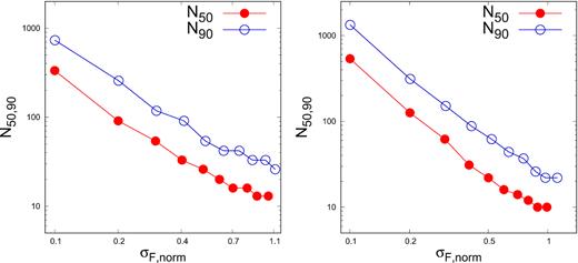
Left-hand panel: The minimum number of bins required, N50 and N90, for 50 per cent and 90 per cent of the light curves to have ΔκF > 0 as a function of normalized standard deviation σF, norm. Right-hand panel: Same as the left one except that the condition is for the AD test, i.e. TSdiff > 0.
Fig. 1 should be interpreted as giving an estimate of the minimum number of bins a light curve should have in order to use skewness to reject the hypothesis that its flux distribution is Gaussian. The minimum number of bins required for 90 per cent of the light curves to have ΔκF > 0 ranges from 25 for σF, norm ∼ 1.1 to 730 for σF, norm ∼ 0.1.
However, from our simulation we found that this is not reliable. The measured value of skewness deviates significantly from the theoretical value for finite number of data points and large σF. The comparison between the observed and theoretical skewness values are given in Appendix A.
Measurement errors of the flux can have a significant impact on the skewness test. If the errors are significant, it would require a larger number of flux points for a distribution obtained from an intrinsically lognormal one, to reject the hypothesis that the distribution is Gaussian. To quantify this effect, we introduce measurement errors that are normally distributed to the simulated light curves. We define a parameter, error ratio, R as the ratio of the sigma of the error distribution σerr to that of the intrinsic flux σF. The measurement error is generated as random normal distribution with standard deviation, σerr = R*σF. We have added this random normal distribution to the intrinsic simulated lognormal light curves. The AD and skewness tests are then applied to the modified lognormal distribution (combination of random noise and intrinsic lognormal distribution). Fig. 2 shows the variation of N90 (left-hand panel) as a function of average normalized standard deviation σF.norm for R = 0.1, 0.5, and 1.0. The figure shows that if the error fraction is larger than 0.5, the number of points in the light curve required to reject the Gaussianity of the distribution is significantly larger than the case when there are no measurement errors.
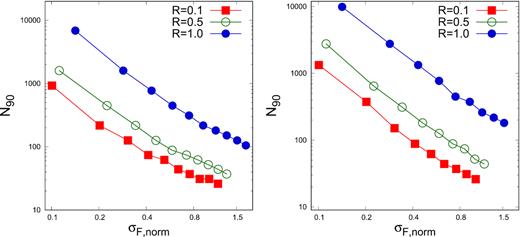
Left-hand panel: Minimum number of flux points, N90, required for 90 per cent of light curves to have ΔκF > 0, are plotted as function of normalized standard deviation σF, norm. The three curves with points shown by colours red (filled square), green (open circle), and blue (filled circle) are for error fraction, R = 0.1, 0.5, and 1, respectively. Right-hand panel: Same as left one except the condition is for the AD test i.e. TSdiff > 0.
Moreover, in some circumstances the measurement error on the flux depends on the flux value, Fi i.e. σerr ∝ Fiα. We have simulated light curves for such cases and show the result for α = 0.1 and 1.0 in Fig. 3. Here, N90 is plotted against σF,norm for R = 0.1 and 1.0. For α = 1.0, the number of points required to reject the Gaussianity is less than for α = 0.
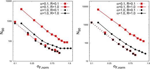
Minimum number of flux bins, N90, as function of normalized standard deviation of flux distribution σF, norm, when the measurement error depends on the flux value. The left-hand and right-hand panels are obtained using skewness and AD tests, respectively. In both panels, black and red curves correspond to α = 0.1 and 1.0, respectively. The dashed and solid representation of curves are for R = 0.1 and 1.0, respectively.
For a lognormal distribution, the skewness and the AD test will accept the normality of the logarithm of the flux at more than 95 per cent confidence level by definition. However, if there is measurement error in the flux, then this may not be so and for sufficiently large error and large number of data points, the test would indicate that the log of the flux distribution is not Gaussian. We simulated light curves with measurement errors and find that when the number of points exceeds 105 (104), the skewness test fails when the error ratio is 0.2 (0.5). Similar results are obtained for the AD test.
As a thumb rule, our results show that both skewness and AD tests can be used to determine that the distribution is not Gaussian, for light curves having more than 100 points and with a normalized standard deviation (fractional rms of variability) greater than 30 per cent. The ratio of the sigma of the measurement error to that of the intrinsic variability should be less than 0.2. The figures presented can be used to gauge the reliability of the tests for other values.
The measurement errors for a light curve can be decreased by binning the light curve in time. Moreover, most measurement processes involve summing the fluxes for a minimum time which is the time resolution of the instrument. While a Gaussian distribution remains a Gaussian one with binning in time, this is not the case for an intrinsically lognormal one. We have performed simulations to illustrate this point quantitatively. We binned simulated light curves from a lognormal distributions such that the resultant binned light curve has 400 data points and a σL ∼ 0.3. The logarithm of the fluxes of these binned light curves was then subjected to the skewness and the AD test, and the fraction of the light curves that failed the tests were noted. This fraction for the skewness and the AD test are plotted as a function of the number points averaged in Fig. 4. It is clear from the figure that binning changes the intrinsic log distribution to some other distribution.
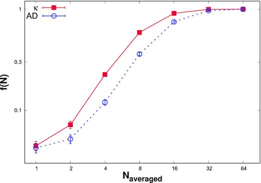
Top panel: The fraction for which lognormality is rejected in the binned flux distribution f(N) as function of the number of flux points over which averaging is done. The solid red curve with filled square points corresponds to skewness test, while the dotted blue curve with open circles corresponds to AD test.
Thus, an intrinsically ‘true’ lognormal distribution that has a white noise power spectrum cannot be determined to be such, if the light curve has been binned. If there is a cutoff in the power spectrum such that there is no intrinsic variability on time-scales shorter than a particular value and if the time resolution is smaller than this value, then the distribution maybe determined to be lognormal. This is further discussed in the last section.
3 SYSTEMS WITH POWER-LAW NOISE
For many physical systems, the power spectra generated from the light curves can be described as a power law i.e. P(f) ∝ f−β. In this section, we explore the efficiency of the skewness and AD tests for such systems. Random time series representing power-law power spectra and whose distribution are Gaussian can be generated using the algorithm proposed by Timmer & Koenig (1995). Using this algorithm, we generated a large sample of light curves for different sets of n and β, the minimum and maximum frequency of the corresponding power-law power spectra are chosen as |$f_{\mathrm{ min}}=\frac{1}{n}$| and fmax = 0.5 , respectively. For β ≤ 1, the time series generated with Timmer & Koenig (1995) algorithm will have Gaussian probability density function (PDF) for all values of n (Morris, Chakraborty & Cotter 2019). However, for steeper power spectral index (β > 1), the light curves become more non-stationary and generated time series are less likely to be described by Gaussian PDF (Alston 2019; Morris et al. 2019). Therefore, in this section we mainly focus on the results for β ≲ 1.
In the previous section, the analysis was based on systems with white noise i.e. for the special case of β = 0. It should be noted that the standard deviation of skewness as well as the critical values for the AD tests are valid only for white noise and cannot be used for the general non-zero β cases. Since we did not find these values in the literature, we first undertook a simulation study to estimate them.
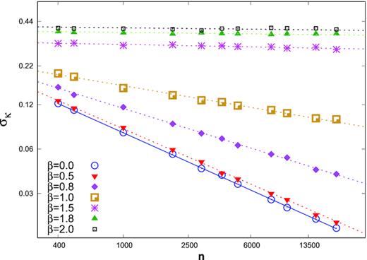
The standard deviation of skewness if plotted against the number of flux points for different values of the power spectrum index β. The solid line is the expected standard deviation |$\sigma _\kappa = \sqrt{6/n}$| valid for the case when β = 0. The dotted lines are the fitted lines using equation (6), with best-fitting values tabulated in Table 1.
Skewness error fit parameters ‘a’ and ‘b’ obtained by fitting the equation (6) to the variation of skewness standard deviation with n for different values of β.
| β | a | b |
|---|---|---|
| 0.0 | 5.96 ± 0.17 | 0.499 ± 0.003 |
| 0.1 | 5.63 ± 0.21 | 0.494 ± 0.003 |
| 0.2 | 6.86 ± 0.25 | 0.513 ± 0.004 |
| 0.3 | 5.89 ± 0.27 | 0.497 ± 0.004 |
| 0.4 | 6.04 ± 0.33 | 0.496 ± 0.005 |
| 0.5 | 5.58 ± 0.24 | 0.482 ± 0.004 |
| 0.6 | 4.54 ± 0.23 | 0.451 ± 0.004 |
| 0.7 | 3.92 ± 0.19 | 0.418 ± 0.004 |
| 0.8 | 1.81 ± 0.18 | 0.345 ± 0.005 |
| 0.9 | 0.58 ± 0.07 | 0.269 ± 0.004 |
| 1.0 | 0.06 ± 0.02 | 0.189 ± 0.005 |
Similarly using 2000 simulated light curves, we estimated the critical values for the AD test for different values of β and significance levels as a function of the number of bins and the results are tabulated in Table 2. As a check, we note that the critical values obtained for β = 0 are similar to those given in literature (written in parenthesis in Table 2).
Critical values of AD test for power-law noise with β = 0.0, 0.5, and 1.0 obtained from simulations. The critical values are obtained at significance level of 15 per cent, 10 per cent, 5 per cent, 2.5 per cent, and 1 per cent.
| Slope (β) | Number of data points (n) | Significance level (per cent) | CV calculated (CV given) |
|---|---|---|---|
| 0.0 | 4096 | 15 | 0.56 (0.575) |
| 0.0 | 2048 | 15 | 0.57 (0.575) |
| 0.0 | 1024 | 15 | 0.56 (0.574) |
| 0.0 | 512 | 15 | 0.56 (0.572) |
| 0.0 | 100 | 15 | 0.55 (0.555) |
| 0.0 | 4096 | 10 | 0.62 (0.655) |
| 0.0 | 2048 | 10 | 0.63 (0.655) |
| 0.0 | 1024 | 10 | 0.63 (0.653) |
| 0.0 | 512 | 10 | 0.63 (0.651) |
| 0.0 | 100 | 10 | 0.68 (0.632) |
| 0.0 | 4096 | 5 | 0.75 (0.786) |
| 0.0 | 2048 | 5 | 0.74 (0.785) |
| 0.0 | 1024 | 5 | 0.75 (0.784) |
| 0.0 | 512 | 5 | 0.75 (0.781) |
| 0.0 | 100 | 5 | 0.75 (0.759) |
| 0.0 | 4096 | 2.5 | 0.88 (0.917) |
| 0.0 | 2048 | 2.5 | 0.87 (0.916) |
| 0.0 | 1024 | 2.5 | 0.89 (0.914) |
| 0.0 | 512 | 2.5 | 0.87 (0.911) |
| 0.0 | 100 | 2.5 | 0.86 (0.885) |
| 0.0 | 4096 | 1.0 | 1.02 (1.091) |
| 0.0 | 2048 | 1.0 | 1.04 (1.09) |
| 0.0 | 1024 | 1.0 | 1.06 (1.088) |
| 0.0 | 512 | 1.0 | 1.03 (1.084) |
| 0.0 | 100 | 1.0 | 1.02 (1.053) |
| 0.5 | 4096 | 15 | 0.58 |
| 0.5 | 2048 | 15 | 0.58 |
| 0.5 | 1024 | 15 | 0.58 |
| 0.5 | 512 | 15 | 0.57 |
| 0.5 | 100 | 15 | 0.56 |
| 0.5 | 4096 | 10 | 0.66 |
| 0.5 | 2048 | 10 | 0.65 |
| 0.5 | 1024 | 10 | 0.65 |
| 0.5 | 512 | 10 | 0.65 |
| 0.5 | 100 | 10 | 0.68 |
| 0.5 | 4096 | 5 | 0.80 |
| 0.5 | 2048 | 5 | 0.79 |
| 0.5 | 1024 | 5 | 0.79 |
| 0.5 | 512 | 5 | 0.78 |
| 0.5 | 100 | 5 | 0.76 |
| 0.5 | 4096 | 2.5 | 0.94 |
| 0.5 | 2048 | 2.5 | 0.93 |
| 0.5 | 1024 | 2.5 | 0.92 |
| 0.5 | 512 | 2.5 | 0.91 |
| 0.5 | 100 | 2.5 | 0.88 |
| 0.5 | 4096 | 1.0 | 1.11 |
| 0.5 | 2048 | 1.0 | 1.12 |
| 0.5 | 1024 | 1.0 | 1.09 |
| 0.5 | 512 | 1.0 | 1.04 |
| 0.5 | 100 | 1.0 | 1.05 |
| 1.0 | 4096 | 15 | 2.62 |
| 1.0 | 2048 | 15 | 2.09 |
| 1.0 | 1024 | 15 | 1.57 |
| 1.0 | 512 | 15 | 1.15 |
| 1.0 | 100 | 15 | 0.69 |
| 1.0 | 4096 | 10 | 3.30 |
| 1.0 | 2048 | 10 | 2.65 |
| 1.0 | 1024 | 10 | 1.95 |
| 1.0 | 512 | 10 | 1.40 |
| 1.0 | 100 | 10 | 0.67 |
| 1.0 | 4096 | 5 | 4.70 |
| 1.0 | 2048 | 5 | 3.72 |
| 1.0 | 1024 | 5 | 2.68 |
| 1.0 | 512 | 5 | 1.64 |
| 1.0 | 100 | 5 | 0.98 |
| 1.0 | 4096 | 2.5 | 5.85 |
| 1.0 | 2048 | 2.5 | 4.83 |
| 1.0 | 1024 | 2.5 | 3.47 |
| 1.0 | 512 | 2.5 | 2.42 |
| 1.0 | 100 | 2.5 | 1.17 |
| 1.0 | 4096 | 1.0 | 7.76 |
| 1.0 | 2048 | 1.0 | 6.67 |
| 1.0 | 1024 | 1.0 | 4.90 |
| 1.0 | 512 | 1.0 | 3.26 |
| 1.0 | 100 | 1.0 | 1.43 |
Having obtained the standard deviation for skewness and the critical values of AD test applicable for light curves having power-law power spectra, we perform similar analysis as was done in the previous section for white noise. In the end of the previous section it was shown that if a light curve having a lognormal distribution and white noise, is binned, the resultant distribution is no longer a lognormal one and both the skewness and AD tests will reject the hypotheses that it is lognormal. We first test the effect of binning on light curves generated from a power-law distribution. We simulated a sample of Gaussian time series using Timmer & Koenig (1995) algorithm, which were exponentiated in order to obtain light curves having lognormal distribution. The exponential model reproduces the observed properties for both stationary and non-stationary light curves (Alston 2019; Alston et al. 2019). It should be noted that the shape of power spectra may not be preserved by exponentiating a time series. However, Uttley et al. (2005) showed that the effect is negligible for PSD’s observed in astrophysical system and it is acceptable to consider the shape of power spectra of lognormal distribution same as that of input linear time series. The generated lognormal light curves are binned in order to have light curves with 400 points and a σL ∼ 0.3. The distribution of the logarithm of the fluxes were tested using skewness and AD tests. In Fig. 6, the fraction of the light curves that failed the tests are plotted as a function of the binning factor. As expected for no binning (Naverage = 1), the fraction fκ and fAD is 0.05 since a 95 per cent confidence has been taken for the tests. As shown earlier, for white noise (β = 0), the fractions increase with binning showing that the distribution is no longer consistent with being a lognormal. However, for β = 0.5 and β = 1.0, the fractions are more or less independent of binning indicating that the lognormal nature is maintained after binning for systems where the power spectrum has a power-law shape with index greater than 0.5. A plausible reason that binning preserves the lognormality could be related to low power in high frequency components for light curve having steeper PSD. The maximum frequency in case of binned light curve can be written as |$f_{\mathrm{ max}}=\frac{1}{2N_{\mathrm{ averaged}}\Delta t}$|, where Δt is the time bin of unbinned (or original) light curve, the maximum frequency decreases as the binning (or Naveraged) increases. In case of steeper PSD, most power is contained in low frequency components and less power will be at higher frequencies. In such cases, the effect of truncation of high frequencies will be less, hence the properties of the original light curve (e.g. lognormal) are preserved. However, in case of white noise, the variability at higher frequencies strongly influence the behaviour of the time series, hence removal of high frequencies from the PSD will change the time series property effectively.
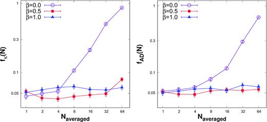
Left-hand panel: The fraction fκ(N) for which lognormality of the binned light curves is rejected (Δκ > 0), plotted against the number of averaged bins. The length of each binned light curve is 400. The three curves viz. violet curve with open circle points, red curve with filled square points, and blue curve with filled triangle points corresponds to the light curves which are generated from power-law noise with β = 0.0, 0.5, and 1.0, respectively. Right-hand panel: Same as the left one except the condition used is for AD test.
We continue the analysis by estimating the minimum number of bins required to reject the hypothesis that the flux distribution of such light curves are Gaussian. The left-hand panel of Fig. 7, displays the minimum number of points required for a lognormal light curve, such that for 90 per cent of them ΔκF > 0, N90, as a function of the normalized standard deviation. The plots are for β = 1.0, 0.5, and 0.0, where β = 0.0 is a repetition of the results obtained in the previous section for white noise. The right-hand panel of Fig. 7, is the same as the left except that it is for the case when TSdiff > 0 for the AD test. We note that the results are similar for β = 0.5 and white noise, but there is marked difference for β = 1.0, where a substantially larger number of bins are required to reject Gaussianity for normalized standard deviations less than 0.5 as compared to white noise. The effect of measurement error is shown in Fig. 8, where N90 as a function of the normalized standard deviation is shown for different values of the error ratio, R for β = 1.0. As expected increasing the ratio of measurement errors to the intrinsic variation, R = σerr/σF), requires a larger number of data points to reject Gaussianity.
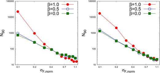
The minimum number of flux points required, N90 such that 90 per cent of the light curve generated will have ΔκF > 0 (left-hand panel) and TSdiff > 0 (right-hand panel) as a function of normalized σF, norm. In both panels, the three curves viz. green curve with filled squares, blue curve with open circles, and red curve with filled circles corresponds to β = 0.0, 0.5, and 1.0, respectively.
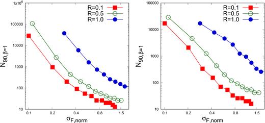
Left-hand panel: Minimum number of flux points, N90, required for 90 per cent of the light curves generated from power-law noise with β = 1.0, to have ΔκF > 0, is plotted as function of normalized standard deviation σF, norm. The three curve’s with points shown by colours red (filled square), green (open circle), and blue (filled circle) are for error fraction, R = 0.1, 0.5, and 1, respectively. Right-hand panel: Same as left one except the condition TSdiff > 0 used is for the case AD test.
Thus, the skewness and AD tests to identify a system have a lognormal distribution that can only be effectively used if the power spectra has an index, β ≳ 0.5, otherwise flux binning would modify the distribution. On the other hand, for large β ∼ 1, the number of bins required to reject the hypothesis that the distribution is Gaussian, is significantly larger (≳1000), than for lower values of β. The most effective analysis can be undertaken when β ∼ 0.5, error ratio R < 0.2, the normalized standard deviation of the light curve is |$\gtrsim 30{{\ \rm per\ cent}}$|, and the number of bins is >100.
4 APPLICATION OF SIMULATION RESULTS ON BLAZAR γ-RAY OBSERVATIONS
The γ-ray flux distribution for a sample of bright Fermi blazars has been studied in detail using skewness, AD test, and histogram fitting by Shah et al. (2018). To check the application of our results derived in Section 3, we consider one of the bright Fermi blazar viz. 3FGL J0730.2−1141 from the sample studied by Shah et al. (2018). Using the skewness and AD tests, Shah et al. (2018) showed that the monthly binned γ-ray flux distribution of this source is lognormal distribution. The number of flux points (after applying quality cuts) in the considered distribution are 99 with normalized standard deviation, σF, norm ∼ 0.68. The skewness, κ and AD TS values of the logarithm of flux distribution are obtained as −0.35 and 0.62, respectively. In order to check the reliability of the AD and skewness tests for confirming the lognormality of flux distribution, we computed the error ratio ‘R’ and power spectra of the monthly binned γ-ray light curve. The R-value for the observed light curve is obtained as 0.0417. We computed the averaged power spectrum by dividing the monthly binned light curve into four segments, each segment of duration 24 months with a binning time resolution of one month. The power-law fit (P(f) ∝ f−β) to the averaged power spectrum, shown in Fig. 9, results in β = 1.02 ± 0.22. Corresponding to β ∼ 1.0 and n = 99, the standard deviation on skewness σκ and |$\mathrm{ cv}_{5{{\ \rm per\ cent}}}$| are obtained as ∼0.25 and ∼0.98 respectively (see Tables 1 and 2). On using the κ, σκ, TS, and |$\mathrm{ cv}_{5{{\ \rm per\ cent}}}$|, the values of Δκ and TSdiff of the logarithm of flux distribution are obtained as −0.15 and −0.36, respectively, both values suggesting the lognormal behaviour of the flux distribution. Further, as shown in Fig. 8, for β ∼ 1, σF, norm ∼ 0.68 and R < 0.1, the available number of flux points, n = 99 are sufficient to satisfy the condition required to reject the Gaussianity of flux distribution at 90 per cent confidence.
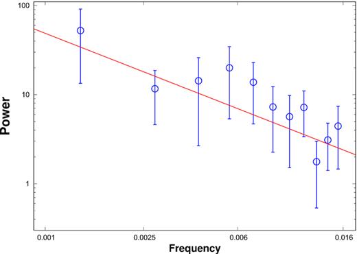
Power spectrum of the monthly binned γ-ray light curve of 3FGL J0730.2−1141. The red solid line is the power-law fit with β = 1.02 ± 0.22.
5 SUMMARY AND DISCUSSION
In this work, using simulations, we have studied the efficiency and reliability of the skewness and AD tests to study whether a light curve corresponds to a lognormal distribution. The tests are used to ascertain whether the light curve’s flux distribution is inconsistent with a Gaussian one, while the distribution of the log of flux is consistent with being a normal distribution. Our motivation is to provide a prescription or guidelines for the effective use of these tests for this endeavour. The recommended prescription is described below, while an example of its implementation is given in the previous section.
(1) For an intrinsically lognormal distribution, the efficiency of the skewness and AD tests to reject that the distribution is a Gaussian one, is similar. The minimum number of bins required in a light curve to reject Gaussianity is nearly equal for both the tests.
(2) It is important to ascertain the nature of the power spectrum of the light curve by estimating the index β of the power law describing the spectrum. If β ∼ 0 (i.e. white noise) then binning changes the distribution and since all light curves are binned to some extent, estimating its flux distribution is meaningless. If β ≳ 1.5, then the variance of the skewness is large and independent of n, and again the skewness and AD tests are not meaningful.
(3) If β ∼ 0.5 or ∼1, then we have provided empirical fits to the standard deviations of the skewness and tabulated critical values for the AD test. These are different from the ones for white noise and we computed them using simulations since we could not find these values in the literature. The skewness standard deviation and critical values can be used to determine significance by which the tests reject that the distribution is normal.
(4) The minimum number of bins required to show that a lognormal distribution is not consistent with a Gaussian one, N90 has been computed as a function of normalized standard deviation and shown in Figs 7 and 8 for different power spectrum index β and levels of measurement error. These can be used a priori to indicate whether a particular observation plan will produce light curves where these tests can be applied. Moreover, if a light curve having larger number of points shows that its flux distribution is consistent with a Gaussian one, then one can say with some confidence that its distribution is not a lognormal one.
(5) The presence of Gaussian measurement errors increases N90 and we recommend that the error ratio, R which is the ratio of the standard deviation of error to the intrinsic standard deviation of flux, to be <0.2. We suggest that the data should be binned in time till R < 0.2. One needs to take care while constructing a histogram for characterizing a PDF shape. The histogram bin width should be chosen such that the width of bin is larger than the measurement error in that bin. Smaller histogram bin width will introduce bias in the shape of PDF, as the flux point with large error cannot be located in single bin. Larger bin width in the histogram will be required for the larger measurement errors, which sometimes produces histogram bins with empty counts. Therefore, in order to reduce the measurement error, one should bin the data till the error ratio, R is optimized. Our work suggest R < 0.2.
(6) For a system having an intrinsic lognormal distribution, the skewness and AD tests will accept the normality of the logarithm of the flux at more than 95 per cent confidence level. However, if there is significant Gaussian measurement error in the flux, the skewness and AD tests may not accept the normality of the logarithm of the flux at 95 per cent confidence level. We show that for an error fraction of R ≲ 0.2, this would require more than 105 data points. Thus for most practical considerations, this effect would be negligible.
(7) The average skewness of the flux of a lognormal distribution differs from its theoretical value for finite number of bins. Moreover, its variance is large. Hence, we do not recommend that the value of the skewness of the flux to be used to show that the distribution is a lognormal one.
This analysis is pertinent to the case when one has a light curve with moderate number of bins say of the order of hundreds. For a larger data set, one can directly fit the histogram of the flux (or the log of the flux) with different distributions to ascertain its nature. Naturally, for a data set with moderate number of bins, the power spectra estimate will not be precise and the power spectra index β would only be known approximately. That is the reason why we have only considered β ∼ 0.5 and 1.0, and not undertaken numerically expensive analysis for finer values of β. This implies that any result obtained from the skewness and AD tests should come with the caveat that they depend on the uncertainty of estimating the power spectrum. For similar reasons, we have not considered the more generic situation when the power spectrum can be described as a broken power law. We note that the variance of the skewness and the AD critical values listed in this work are for power-law power spectra and are not applicable for a broken power law. For typical cases, where a flat power spectrum (e.g. β ∼ 0.5) breaks into a steeper one (e.g. β ∼ 1.5) beyond a break frequency, we recommend that the light curve be rebinned to a bin size corresponding to the break frequency and then apply the skewness and AD tests. Since the power-law index is typically steep beyond the break frequency, rebinning will not lead to significant loss of information and in general will decrease the measurement noise level.
As an important aside, we have addressed a conceptually paradoxical issue regarding non-Gaussian flux distributions. While Gaussian distributions remain Gaussian on addition, i.e. Gaussian flux distribution remain Gaussian when the light curve is rebinned, this is in general not true for other distributions such as a lognormal one. Thus, it is not clear why several astrophysical systems display lognormal distributions when the light curves they are estimated from, are always binned to some time bin. We resolve this issue by showing that if the power spectra of the light curves can be described by a power law with index β ≳ 0.5, then the nature of the distribution is invariant to rebinning. Thus for a system to be scale free in time and have a lognormal flux distribution its power spectra must be steeper than 0.5. This insight may have important consequences for the model development and understanding of systems with lognormal distributions.
Understanding the nature of flux distribution using first analysis tools like skewness and AD that can be applied to moderate size data sets, is an important step laying the foundation for more elaborate studies. The results presented here provide a prescription and guidelines for the effective and reliable use.
ACKNOWLEDGEMENTS
We thank the anonymous referee for his critical assessment of our work. The referee comments and suggestions have helped us in improving this manuscript. We thank a UGC-UKIERI Thematic Partnership for support. We acknowledge the use of Fermi-LAT data provided by Fermi Science Support Center (FSSC).
DATA AVAILABILITY
The Python codes and data used in this article will be shared on reasonable request to the corresponding author, Zahir Shah (email: [email protected] or [email protected]).
REFERENCES
APPENDIX A: SKEWNESS
A possible way to test the lognormality of a flux distribution is to compare the computed skewness of the distribution with the theoretical value given by equation (4). However, we find that for a moderate number of data points of hundreds, this is not a reliable method. We simulated light curves corresponding to a lognormal flux distribution for different sets of σLF and n (see Section 2 for details), 10 000 light curves for each set of σLF and n. We measured the skewness value κF for all such light curve, and calculated their average, |$\bar{\kappa }_F$|. Fig. A1 shows |$\bar{\kappa }_F$| as a function of σF, norm using dotted lines with symbols representing different lengths of the light curve, n. The solid curve is the theoretical skewness calculated using equation (4). The figure clearly shows that |$\bar{\kappa }_F$| is significantly smaller than the theoretical values for small n and this deviation increases with the standard deviation of the light curve. Only asymptotically with large n does |$\bar{\kappa }_F$| match with the theoretical values. Thus, comparison of the computed skewness with the theoretical value cannot be done, for moderate length light curves. While it is possible to empirically fit the expected |$\bar{\kappa }_F$| as a function of n and normalized flux standard deviation, σF, norm, this may not be warranted because of the large variation of κF. This is shown in Fig. A2, where the standard deviation of the skewness (normalized by the average) is shown as function of σF, norm for different n. For n < 1000, the variation of κF is always more than 20 per cent, which will not allow for any meaningful inference.
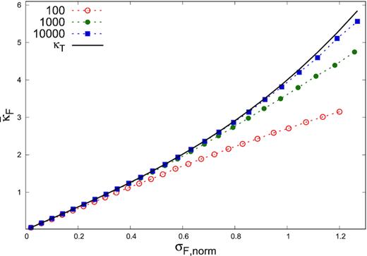
Average of the skewness of flux distribution (|$\bar{\kappa }_F$|) against normalized standard deviation of flux distribution σF, norm. The solid curve with black colour corresponds to the theoretical curve. The dotted curves are for different values of length of light curve, n.
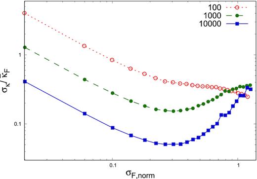
The standard deviation of the skewness divided by the mean of skewness (|$\sigma _\kappa /\bar{\kappa _F}$|) versus the normalized standard deviation of flux distribution σF, norm for n = 100, 1000, and 10 000.
