-
PDF
- Split View
-
Views
-
Cite
Cite
Berta Margalef-Bentabol, Marc Huertas-Company, Tom Charnock, Carla Margalef-Bentabol, Mariangela Bernardi, Yohan Dubois, Kate Storey-Fisher, Lorenzo Zanisi, Detecting outliers in astronomical images with deep generative networks, Monthly Notices of the Royal Astronomical Society, Volume 496, Issue 2, August 2020, Pages 2346–2361, https://doi.org/10.1093/mnras/staa1647
Close - Share Icon Share
ABSTRACT
With the advent of future big-data surveys, automated tools for unsupervised discovery are becoming ever more necessary. In this work, we explore the ability of deep generative networks for detecting outliers in astronomical imaging data sets. The main advantage of such generative models is that they are able to learn complex representations directly from the pixel space. Therefore, these methods enable us to look for subtle morphological deviations which are typically missed by more traditional moment-based approaches. We use a generative model to learn a representation of expected data defined by the training set and then look for deviations from the learned representation by looking for the best reconstruction of a given object. In this first proof-of-concept work, we apply our method to two different test cases. We first show that from a set of simulated galaxies, we are able to detect |${\sim}90{{\ \rm per\ cent}}$| of merging galaxies if we train our network only with a sample of isolated ones. We then explore how the presented approach can be used to compare observations and hydrodynamic simulations by identifying observed galaxies not well represented in the models. The code used in this is available at https://github.com/carlamb/astronomical-outliers-WGAN.
1 INTRODUCTION
In recent years, the amount of astronomical data produced both by observations and simulations has exponentially increased in volume and complexity. This trend is expected to continue in the near future with surveys such as LSST and EUCLID becoming available. Processing and extracting meaningful physical information from these new data sets is a new challenge for the community.
To provide the necessary computational relief, machine learning techniques are becoming more and more popular as a way to address the increasing complexity. In particular, supervised machine learning has proven to be very successful when large amounts of labelled or annotated data are available for classification (e.g. Huertas-Company et al. 2015; Cabrera-Vives et al. 2017; Jacobs et al. 2017; Kim & Brunner 2017; Domínguez Sánchez et al. 2018; Huertas-Company et al. 2018; Sreejith et al. 2018; Davidzon et al. 2019), regression (e.g. Tuccillo et al. 2018; Bonjean et al. 2019; Pasquet et al. 2019), and segmentation (e.g. Boucaud et al. 2020).
Supervised algorithms rely on annotated data sets and are thus, not well suited to the discovery of new types of unknown objects which will certainly be present in future surveys. In order to fully unlock the discovery potential of machine learning we have to leverage unlabelled data. Unsupervised algorithms aim to learn the underlying distribution of the data and find patterns without relying on annotated data. Such unsupervised methods can be, hence, used to detect objects whose properties deviate from the expected or normal objects given a data distribution. These abnormal objects are commonly referred to as outliers or anomalies. Anomaly detection is an active field in machine learning and has a broad range of applications ranging from fraud detection to surveilance (e.g. Frery et al. 2017; Zhang, Vukotic & Gardner 2018) to early diagnosis of disease outbreaks (Wong et al. 2005).
In astronomy, outliers can represent artifacts in the data, pipeline errors or new physics. In the case of data or pipeline artifacts, it is important to further analyse them to better reduce systematics. On the other hand, any novel findings can potentially lead to interesting new science (Norris 2017) or objects which differ between models and observations. Several machine learning methods have already been successfully applied to detect outliers in astrophysical data sets, such as unknown classes of objects or objects belonging to rare classes. For example, self-organizing maps have been used to detect unusual quasars (Fustes et al. 2013) and spectroscopic outliers (Meusinger et al. 2012), random forests have been used to detect anomalous SDSS spectra (Baron & Poznanski 2017), one-class support vector machines have been employed for novel detection in the WISE survey (Solarz et al. 2017) and clustering algorithms have been utilized to detect anomalous data in light-curves (Protopapas et al. 2006; Giles & Walkowicz 2018).
Anomaly detection in astronomical images is, however, a more complex task because of the high dimensionality (i.e. high number of parameters, in this case the number of pixels in the image) and limited amount of data. Traditional machine learning approaches, such as those mentioned earlier, typically rely on some reduced set of summary statistics (such as photometry, spectroscopic features, or shape measurements), which usually discard a large amount of information about the image complexity and, therefore, can miss some subtle morphological anomalies. Deep generative models, on the other hand, are a modern class of unsupervised methods with the ability to learn complex representations of high-dimensional data in such a way that they can generate new examples drawn approximately from the same distribution as the original data set. Generative Adversarial Networks (GANs; Goodfellow et al. 2014) provide a framework for training such deep generative models. They have gained popularity in recent years for their ability to produce extremely realistic images of everyday scenes (Radford, Metz & Chintala 2015; Karras et al. 2018) and have also been used in astronomy to generate realistic galaxy images (Ravanbakhsh et al. 2017). Recently, work has shown that GANs can be efficiently used for anomaly detection in medical image data sets (Schlegl et al. 2017; Murphy et al. 2018). They present a promising application for anomaly detection in astronomical images. One of the key advantages of a generative model-based approach for anomaly detection is that the model can learn to represent complex data directly from the pixel distribution without relying on specific galaxy properties, that could, otherwise, introduce biases from the methods used to obtain such properties.
This work, as the first in a series of studies, aims to achieve two goals: to test of the ability of generative models to identify outliers in astronomical imaging data sets (i.e. images that are significantly different to the expected or ‘normal’ data) and their capability to globally discern differences between data sets. To address the first goal, we test the approach in a well-defined sample of simulated galaxies from the cosmological hydrodynamic simulation Horizon-AGN (Dubois et al. 2014). We define isolated galaxies as the normal objects and then quantify how frequently merging galaxies are detected as outliers. We chose this example for the potential to have a large sample of well-defined anomalies (the mergers) and therefore the ability to draw statistically significant conclusions. For that reason, in this first test, we refrain from testing our method with human-labelled anomalies on real data, as the sample of anomalies would not be sufficiently large. For our second task, we explore whether Wasserstein GANs (WGANs, discussed in Section 3.3; Arjovsky, Chintala & Bottou 2017; Gulrajani et al. 2017) can be employed to quantify differences between observations and simulations.
The paper is structured as follows: In Section 2 we present the data we use for this work. In Section 3 we explain the methodology for anomaly detection. Section 4 is devoted to describing different possible applications. And finally, we summarize our findings in Section 5.
2 DATA
For this work, we use both simulated data from the Horizon-AGN cosmological hydrodynamical simulation (Dubois et al. 2014) and observed galaxies from the CANDELS survey (Grogin et al. 2011; Koekemoer et al. 2011).
2.1 Horizon-AGN
We refer the reader to Dubois et al. (2014) for complete details of the simulation suite. Horizon-AGN is a cosmological hydrodynamical simulation run in a |$L_\textrm{box} = 100 \, h^{-1} \, \textrm{Mpc}$| cube with initial conditions drawn from WMAP-7 cosmological parameters (Komatsu et al. 2011). The total volume contains 10243 dark matter (DM) particles, with a DM mass resolution of |$M_\textrm{DM,res} = 8\times 10^7 \, \mathrm{M}_{\odot }$|. The simulation is run with the adaptive mesh refinement code ramses (Teyssier 2002), and the initially uniform grid is refined down to a minimum cell size of |$1\, \textrm{kpc}$| constant in physical length. Gas is allowed to cool down to 104 K through H and He collisions with a contribution from metals using a Sutherland & Dopita (1993) model. Gas is heated from a uniform UV background after zreion = 10 following Haardt & Madau (1996). Star formation occurs in regions where the gas density reaches a critical density of |$n_0=0.1\, \textrm{H}\, \textrm{cm}^{-3}$| and it is modelled with a Schmidt law: ρ* = ϵ*ρ/tff, where ρ* is the star formation rate density, ρ is the gas density, ϵ* = 0.02 (e.g. Kennicutt 1998) the constant star formation efficiency and tff is the local free-fall time of the gas. Stellar feedback is included assuming a Salpeter (1955) initial mass function (IMF), and occurs via stellar winds, supernovae type II and type Ia, with mass, energy, and metal release of six chemical species: O, Fe, C, N, Mg, and Si. Black hole (BH) feedback is also included in the simulation as modelled in Dubois et al. (2012), with BHs releasing energy in a quasar (heating) mode for a high accretion rate (Eddington ratio >0.01) and in radio mode (jet) for low accretion rates (Eddington ratios <0.01).
In Horizon-AGN, galaxies are identified using the AdaptaHOP structure finder (Aubert, Pichon & Colombi 2004) over the stellar distribution. The merger trees for the identified galaxies are built using the procedure outlined in Tweed et al. (2009), considering 758 time-steps that cover a redshift range spanning from z = 7 to z = 0 and with a time difference of 17 Myr in average between two successive time-steps.
2.1.1 Mock images
From the output of the simulation, we produce mock observations that will be used to train the generative models. In particular, mock images are produced to replicate the properties of the HST-CANDELS images in the H-band (F160W), using the sunset code (e.g. Kaviraj et al. 2017; Laigle et al. 2019), which models the emission of all galaxy particles to produce an image in the observed-frame. For each identified galaxy in the simulation, we define a cubic volume centred around the galaxy with an edge length of eight times the radius of the galaxy (in this case, defined as the average between the three semi-axes obtained when fitting an ellipsoid to the stellar mass distribution of the galaxy). This volume should contain the stellar particles from the main galaxy as well as those from any close companion, in order to capture any secondary progenitor in the image for the case of galaxy mergers. The stellar particles contained within the volume are used as an input to sunset, along with the spectral response of the H-band filter of the WFC3 camera. sunset computes the fluxes corresponding to the inputs using the stellar models of Bruzual & Charlot (2003) and a Chabrier (2003) IMF. It is assumed that each particle is well described by a simple stellar population, for determining the contribution of each particle to the Spectral Energy Distribution (SED). For this work, we chose not to include dust effects in the image generation for computational reasons. This should not be a problem for tests involving only simulated data but can significantly affect the comparison with observations. We will discuss this in Section 4.2.2. Finally, the integration of the SED in each pixel and the redshift of the galaxy are used to generate an image in the observed frame. The physical size of the pixel is re-scaled for every image to 0.06 arcsec, to match the resolution of the CANDELS H-band images. The flux is then scaled using the H-band zero-point of CANDELS to match the S/N. Finally, to generate a realistic mock observation, the rescaled images are convolved with the corresponding PSF. These steps are repeated for three different projections along the main axis of the simulations (X,Y,Z) so that for every 3D cube three images are produced. The final sample built that way consists of 1524 118 mock images which include all galaxies with log (M*/M⊙) > 10 and 0.5 < z < 3, with 250 snapshots in the redshift range. For the purpose of this work, we set a fixed image size of 64 × 64 pixels.
2.2 CANDELS
We use H-band images from the five CANDELS (Grogin et al. 2011; Koekemoer et al. 2011) fields: UDS, COSMOS, GOODS-S, GOODS-N and EGS. The parent sample comes from the catalogue of Dimauro et al. (2018). Our final selection is made of H-band selected galaxies with magnitudes brighter than F160 = 23.5, log (M*/M⊙) > 10 and 0.5 < z < 3, to match the sample of galaxies from the Horizon-AGN simulation in stellar mass and redshift. The final sample consists of 17 611 CANDELS images.
We use the official catalogues of redshifts (spectroscopic redshifts are used when available) and stellar masses from CANDELS. The UDS and GOODS-S photometric redshifts were determined using the method described in Dahlen et al. (2013). Stellar masses are drawn from the catalogue presented in Santini et al. (2014) using these photometric redshifts. For the COSMOS, GOODS-N, and EGS fields, the photometric redshifts and stellar masses are discussed in Nayyeri et al. (2017), Barro et al. (2019), and Stefanon et al. (2017), respectively.
We additionally use the structural parameters (Sérsic index, n, effective radius, Reff, and axial ratio, q) published in Dimauro et al. (2018), obtained from 2D single Sérsic fits on the H-band (F160W), and the deep-learning based visual morphologies from Huertas-Company et al. (2015).
3 METHOD
3.1 Deep neural networks
Artificial Neural Networks (ANN; Hassoun 1995), are computational techniques vaguely inspired by the connections that are established between the neurons in the brain and their ability to store and process information. An ANN consists of a collection of connected nodes or units (or neurons). The connections (or synapsis) are directed and have associated weights. Those weights are determined by training (or learning).
The nodes of a network are typically arranged in layers. The particular arrangement of the nodes into layers and the connection patterns between them is called the architecture of the neural network. Input layers contain the nodes that receive their input from an external source, output layers provide the output of the network, and the layers in between are referred to as hidden layers. Each node of the hidden layers (hidden unit) is a mathematical function that receives inputs from units in the previous layer and computes an output that is transmitted to other units in the next layer based on the connecting weights. The goal is to use the network as a complex non-linear function that provides some desired output for each input. A cost function or loss is defined to quantify how far is the desired output from the network’s actual output. Training is the process of determining the best set of weights to minimize the cost function for a given data set.
Deep-learning Networks (or Deep Networks) are ANNs comprised of many more hidden layers than traditional ANNs and typically have more complex architectures and mathematical functions in their units. Convolutional Neural Networks (CNNs) are a particular architecture of deep networks that were developed within the context of image processing and computer vision applications (Fukushima 1988). CNNs are comprised of one or more convolutional layers followed by one or more fully connected layers. The convolutional layers take as input a set of feature maps (e.g. the colour channels of an image) and convolve each of these with a set of learnable filters to produce the output feature maps. Each layer adds more abstraction to the original input and produces a more informative set of features for the next layer. The fully connected layers have every node in a layer connected to every node in the following layer. They act as a classifier, taking as input the features from the last convolutional layer. The architecture of a CNN is designed to take advantage of the 2D structure of an input image, preserving the spatial relationship between pixels, i.e. they are able to learn translationally invariant features from the data. By exploiting the translational symmetry of the data, CNNs have shown to produce great results for pattern recognition in images.
3.2 Generative advesarial networks, GANs
Generative adversarial networks (GANs) were first introduced in Goodfellow et al. (2014). In the original formulation, they consist of two networks that are trained simultaneously: a generator (the generative model to be trained) and a discriminator (a classification model). The generator, Gθ, with parameters |$\boldsymbol{\theta }$|, produces new samples from the approximated target data distribution whilst the discriminator, Dψ, with parameters |$\boldsymbol{\psi }$|, aims to distinguish the generated samples from the true target distribution.
3.3 Wasserstein generative adversarial networks, WGANs
3.4 Training procedure
We implement CNN architectures for the critic and the generator, both shown in Fig. 1. The generator network takes as input a random vector of size 100 and outputs an image of size 64 × 64 pixels. It consists of one dense layer and six convolutional layers. The critic consists of five convolutional layers and two dense layer. It takes as input an image of 64 × 64 pixels and outputs a real number. The final architectures used in this work have been achieved through manual optimization and will not necessarily suit other applications.

Critic (top) and generator network (bottom). The critic in this work consists of five convolutional layers and two dense layers. It takes as input an image of 64 × 64 pixels and outputs a real number. The generator network is made of one dense layer and six convolutional layers. It takes as an input a random vector of size 100 and outputs an image of size 64 × 64 pixels.
The WGAN is trained following the standard procedure outlined in Gulrajani et al. (2017). Similar to the original GAN, the two networks of the WGAN are trained alternately. A schematic representation of the WGAN training is shown in Fig. 2. We use a default value of λ = 10 for the gradient penalty coefficient, a number of critic iterations per generator iteration ncritic = 10, batch size m = 32 and Adam optimizer with the following hyperparameters: α = 0.00005, β1 = 0.5, β2 = 0.9. We use keras1 with tensorflow2 as the backend. The exact algorithm is shown in Appendix A.
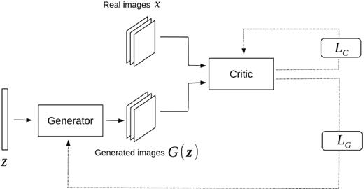
Schematic representation of the WGAN training. Given a batch of real and generated images, the critic is trained for ncritic iterations to approximate the Wasserstein distance, by minimizing Lc whilst keeping the weights of the generator fixed. Afterwards, the generator’s weights are updated for a single iteration, whilst the critic weights are held constant so that it minimizes the approximate Wasserstein distance.
3.5 Anomaly detection method
Our goal is to use the trained WGAN to detect outliers. The main underlying idea is that after training is completed, the generator Gθ should be able to take a point |$\boldsymbol{z}$| from the latent space and generate an image that resembles the images used for training (normal images). However, whenever an image does not come from the distribution of normal images then it will not be possible to generate a similar image from any point, |$\lbrace \boldsymbol{z}|\boldsymbol{z}\in \mathbb {R}^{N_z}\rbrace$|, in the latent space, |$\mathbb {R}^{N_z}$|, and it will be in some sense anomalous.

Schematic representation of the anomaly detection training. The grey colour represents that the weights of a network are fixed during training. Given a real image and a noise vector, the network μ finds the anomaly score and the closest generated image by minimizing the combined loss LA (see equation 6) whilst keeping the weights of the generator and critic fixed. The critic features box represent the critic network without the last two dense layers, and it outputs a feature map obtained before the fully connected layers.
The procedure is not optimal from a performance perspective since images need to be processed individually. It can easily be improved by performing a global optimization over multiple images and then applying a simple gradient descent to refine as shown in Storey-Fisher et al. (in preparation). Since computing time is not critical for this work in which the sample of images to test is not enormous, we keep this original implementation.
Note that, whilst the anomaly score does not have a true meaning independent of the training of each of the critic, the generator and μϕ, anomalous data can be identified by comparing it to the distribution of the training data, which the generator is trained to approximately draw from. For this reason, we measure the anomaly score for all the images in our training set which acts as the calibration of the anomaly detector. Any new image with an anomaly score significantly outside the bulk of scores for the training images is then quantified as being, in some way, anomalous.
4 APPLICATIONS
In the following section, we explore several cases in astronomy for our WGAN-based anomaly detector. We first calibrate how the anomaly detector performs with a sample of known anomalies. In particular, we quantify how accurately images of mergers are detected as anomalous when our training sample (the ‘normal’ sample) is a set of isolated galaxies. We split this application in two cases: the first case focuses on detecting anomalies due to the presence of a neighbour object, and the second one focuses on analysing more subtle merger-induced morphological disturbances. The last application consists of using the anomaly score to compare a sample of images from the Horizon-AGN simulation to real galaxies from the CANDELS survey, to quantify the difference or similarity between such data sets.
4.1 Galaxy mergers as anomalies
4.1.1 Training
The training set consists of images of isolated galaxies (no mergers), which we call the ‘normal images’, and the test set consists of images of galaxy mergers. The selection of interacting galaxies in the simulations is done by checking an increase in galaxy mass due to the contribution of more than one progenitor from the previous time-step (Rodriguez-Gomez et al. 2015; Abruzzo et al. 2018). If a galaxy has more than one progenitor and the ratio between the stellar mass provided by the secondary and the main progenitor is equal or larger than 1:10, then that galaxy will be considered a merger. When a merger is identified, we build a merger sequence by going back in time in the merger tree until the companion is four effective radii away from the central galaxy. We call all these images pre-mergers. We also follow forward in time after the merger event for the same number of time-steps. These images are called post-mergers.
Isolated galaxies, on the contrary, satisfy the condition of having only one progenitor when going back in time 1 Gyr and only one descendant when going forward in time 1 Gyr. Images for both data sets are generated as explained in Caro (2018). The final training sample is made of 531 922 isolated galaxies. Examples of these images are shown in Fig. 4. We also show the stellar mass and redshift distributions for our training and test samples in Fig. 5. Notice that the distributions are significantly different given the restrictive constraints used to define the sample of isolated galaxies. By imposing no interactions in a 2 Gyr time window we remove very massive galaxies from the sample. This is not a problem since we are aiming to calibrate the sensitivity of the WGAN anomaly detector in identifying out-of-distribution objects. It should be noted that mergers are not anomalous scientifically speaking but are outside of our training data and as such we want to detect them.
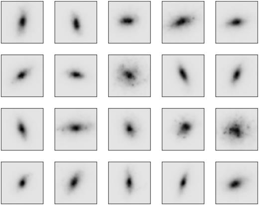
Examples of mock images (observed in the H-band) from the Horizon-AGN simulation that are used as training data. The images have a size of 64 × 64 pixels, and the pixel scale is 0.06 arcsec pixel−1.

Stellar mass (left-hand panel) and redshift distribution (right-hand panel) of the training data (isolated galaxies in striped green and mergers images in solid yellow). We can see obvious deviations between the distributions of isolated galaxies and mergers which should be quantifiable as anomalous by the anomaly WGAN detector.
We train a WGAN network, described in Section 3.3 for ∼×106 epochs using only isolated images. As a first exploratory step, Fig. 6 shows some examples from the test set indicating their anomaly score, the closest generated image, and the residual image (derived by subtracting the closest generated image to the original image). We see that for images with low anomaly score values, the residuals are low as expected, due to the network being able to generate very similar images. For high anomaly score images, the residuals are larger because the network cannot generate a similar image. In several cases, the anomaly is due to the presence of a secondary source as one would naturally expect. Fig. 7 shows a 2D representation of the last layer of the critic (which is used to compute LF) computed with t-Distributed Stochastic Neighbour Embedding (t-SNE; van der Maaten & Hinton 2008). t-SNE is a technique for dimensionality reduction that helps with the visualization of high-dimensional data sets. In the high dimensional space, it models the probability distribution that dictates the relationships between neighbours around each point. Then in the low-dimensional space, it recreates, as close as possible, the same distribution. When points are close to one another in the high-dimensional space they will tend to be close to one another in the low-dimensional space as well. Notice that the axis of the low-dimensional space are arbitrary and have no particular interpretation. We show a subsample of normal galaxies and a subsample of galaxies with a neighbour in the image. This visualization suggests that the network is well trained for our purpose, and the critic is, indeed, able to separate these two classes well. Therefore, using the critic as part of the anomaly score should provide information with which we can detect anomalies. The next sections quantify the performance.
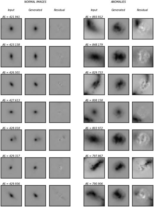
Examples of images draw from the test sample with low anomaly score (left-hand panel) and high anomaly score (right-hand panel). In the first column, we show the input image, in the second column, the closest generated image obtained in the anomaly detection method, and in the third column, the residual (pixel by pixel difference) between the input and the generated. The normal images show low anomaly score values and a very similar image can be generated by the network. For the test images the anomaly score is high and no close image can be generated which results in large residuals.

Output of the last convolutional layer of the trained critic after reducing it to two dimensions using the t-Distributed Stochastic Neighbour Embedding method (noting that this is just one realization of the t-SNE). We show where normal images (purple) and images of galaxies with neighbours (green, images that are most different to the normal set) lay in this plane.
4.1.2 Results: anomalies caused by a companion in the image
We now quantify how accurately we can detect anomalies due to the presence of a companion in the image. Given that our training sample consists of isolated galaxies, we can assume that the presence of a secondary object will contribute the most to the degree of anomaly on an image when compared with the training sample.
We, therefore, select all the images with at least a secondary object in the image (this will be our known anomalous sample in this application). All these images belong to the pre-merger phase. However, not all pre-mergers have a secondary object in the image. This is because, in order to speed up the training process and due to memory capability, we have cropped the original images from the simulations to 64 × 64 pixels, and therefore, in some cases, we have artificially removed the companion object that will eventually merge with the main galaxy.
We compute the anomaly score for the training sample as well as for the test sample and compare their distributions in Fig. 8. The figure clearly shows that the AS distribution for mergers peaks at larger values than the one for isolated galaxies. To quantify the anomaly detection method, we define a threshold-based method. Images that have an AS larger than the threshold are considered anomalous (or inconsistent with the training sample), while images with AS lower than the threshold, are considered ‘normal’ (or consistent). We use three different thresholds defined as the value that contains 85, 90, and 95 per cent of the training galaxies within the generative distribution. Using these thresholds, we find 86, 80, and 67 per cent of the anomalous samples are correctly identified as anomalies, respectively. We compare our results with a more traditional method of outlier detection, the k-means clustering method (MacQueen 1967). For that, we use non-parametric measures of structure used to quantify the broad morphology: CAS (concentration C, asymmetry A and clumpiness S; Conselice 2003), and Gini/M20 parameters (e.g. Abraham, van den Bergh & Nair 2003; Lotz, Primack & Madau 2004). We calculate these parameters for the two samples (training and test) using the code statmorph, a python package for calculating non-parametric morphological diagnostics of galaxy images (Rodriguez-Gomez et al. 2019), and apply the k-means method with two clusters. We find that 99 per cent of the training sample belongs to one cluster while 74 per cent of the pre-mergers with a neighbour lie in the other cluster. These results are summarized in Table 1.

Anomaly score distribution for the isolated galaxies (training data, purple) and the pre-mergers with neighbours (green). The black dash, solid, and dotted line represent the three thresholds defined as the value that, respectively, contain 85, 90, and 95 per cent of the training galaxies within the generative distributions. The distribution for the pre-mergers peaks at a higher value than the training data, with clear separations between the distribution. This indicates that the majority of pre-mergers with neighbours are inconsistent with the training sample.
Accuracy of the threshold-based anomaly detector for different thresholds, and of k-means anomaly detector method. Each method (columns) is evaluated for test sets (rows) of isolated and pre-merger galaxies. Thresholds 1, 2, and 3 represent the three thresholds defined as the value that contains, respectively, 85, 90, and 95 per cent of the training galaxies within the generative distribution. The last column indicates the accuracy according to the k-means clustering method.
| Accuracy of the anomaly detector . | ||||
|---|---|---|---|---|
| . | Threshold . | . | ||
| . | 1 . | 2 . | 3 . | k-means . |
| Isolated | 85 per cent | 90 per cent | 95 per cent | 99 per cent |
| Pre-mergers | 86 per cent | 80 per cent | 67 per cent | 74 per cent |
| Accuracy of the anomaly detector . | ||||
|---|---|---|---|---|
| . | Threshold . | . | ||
| . | 1 . | 2 . | 3 . | k-means . |
| Isolated | 85 per cent | 90 per cent | 95 per cent | 99 per cent |
| Pre-mergers | 86 per cent | 80 per cent | 67 per cent | 74 per cent |
We further investigate the incorrectly classified pre-merger galaxies, and find that the majority of these are caused by a high flux ratio between the main galaxy and the brightest neighbour. We hence compute the flux ratio Fr between the main galaxy and the companion using sextractor (Bertin & Arnouts 1996) and then divide the test sample into three bins depending on the flux ratio (Fr < 1.5, 1.5 < Fr < 2, Fr > 2). For flux ratios lower than 1.5, we find that 96, 93, and 86 per cent are correctly classified as anomalous, using the three thresholds mentioned above, respectively. For galaxies between 1.5 and 2 times as bright, there is only a small decrease in these percentages (94, 90, and 76 per cent). It is only when the companion is 2 times fainter than the central galaxy (46 per cent of our test sample) that the percentage of galaxies correctly classified drops to 75, 66, and 48 per cent, respectively, for the three different thresholds. We find that while for Fr < 1.5 and 1.5 < Fr < 2, our results are comparable to the k-means method (91 and 93 per cent of the test sample are correctly classified according to the k-means method), when considering galaxies with a companion two times fainter, the k-means method performs significantly worse at detecting them as anomalous (only 39 per cent, compared with 75, 66, and 48 per cent, respectively, for the three different thresholds used in our method). These results are summarized in Table 2. We have also explored whether the distance between the main galaxy and the companion has an effect on the anomaly score, but we have found no correlation.
Accuracy of the threshold-based anomaly detector for different thresholds, and of k-means anomaly detector method. Each method (columns) is evaluated for test sets (rows) of pre-merger galaxies divided according to their flux ratio between the central galaxy and the brightest neighbour (Fc/Fn). Thresholds 1, 2, and 3 represent the three thresholds defined as the value that contains, respectively, 85, 90, and 95 per cent of the training galaxies within the generative distribution. The last column indicates the accuracy according to the k-means clustering method.
| Accuracy of the anomaly detector . | ||||
|---|---|---|---|---|
| . | Threshold . | . | ||
| . | 1 . | 2 . | 3 . | k-means . |
| Fr < 1.5 | 96 per cent | 93 per cent | 86 per cent | 91 per cent |
| 1.5 < Fr < 2 | 94 per cent | 90 per cent | 76 per cent | 93 per cent |
| Fr > 2 | 75 per cent | 66 per cent | 48 per cent | 39 per cent |
4.1.3 Results: anomalies caused by merger induced morphological perturbations
In the previous section, we have seen how the anomaly detection method is able to detect anomalous galaxies with high accuracy when a relatively bright companion is found in the image. Here we investigate how accurately the method works when the companion is not present (i.e. for the pre-merger galaxies that do not show a neighbour object in the image and images of the post-merger phases). This exercise is intended to test the robustness of the WGAN-based anomaly detector given more subtle merger-induced perturbations in the main galaxy light distribution. For this application our anomalous sample, therefore, consists of galaxies in the pre-merger phase that do not have a neighbour object as well as galaxies in the post-merger phases.
Fig. 9 shows the anomaly score distributions for isolated pre-mergers (or pre-mergers without neighbours) and post-mergers. As expected, we observe that even if both samples have anomaly score distributions extending to larger values than the training set, the majority of the samples overlap with the training data. Using the same three thresholds as before, 46, 39, and 30 per cent of these images are classified correctly (respectively for the three thresholds), while only 8 per cent when using the k-means clustering method. Overall, it appears the isolated pre-mergers are detected as anomalous slightly more often than the post-mergers. We summarize these results in Table 3. These results indicate that the presence of a secondary object is not the only cause of anomaly in these images, although it is the dominating factor, and that the WGAN is able to detect more subtle morphological differences between the samples. Our results also demonstrate the WGAN method is better suited to finding outliers than traditional clustering methods, particularly when the differences with the training sample are subtle and cannot be fully described by global measures, as they are in this case. We further investigate what features describe the difference between the anomalous images and the training set.
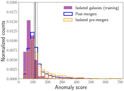
Anomaly score distribution for the isolated galaxies (training data, purple), the isolated pre-mergers (orange), and post-mergers (blue). The black dash, solid, and dotted line represent the three thresholds defined as the value that contain, respectively, 85, 90, and 95 per cent of the training galaxies within the generative distribution. The distribution for the isolated pre-mergers and post-mergers (test sample) extend to larger values than the training data, even though there is significant overlap between the distribution. There are many samples which are inconsistent with the training data.
Accuracy of the threshold-based anomaly detector for different thresholds, and of k-means anomaly detector method. Each method (columns) is evaluated for test sets (rows) of isolated pre-mergers, post-merger galaxies, and the combinations of both sets. Thresholds 1, 2, and 3 represent the three thresholds defined as the value that contain, respectively, 85, 90, and 95 per cent of the training galaxies within the generative distribution. The last column indicates the accuracy according to the k-means clustering method.
| Accuracy of the anomaly detector . | ||||
|---|---|---|---|---|
| . | Threshold . | . | ||
| . | 1 . | 2 . | 3 . | k-means . |
| Isolated pre-mergers+Post-mergers | 46 per cent | 39 per cent | 30 per cent | 8 per cent |
| Isolated pre-mergers | 52 per cent | 45 per cent | 37 per cent | 7 per cent |
| Post-mergers | 45 per cent | 38 per cent | 28 per cent | 9 per cent |
Fig. 10 shows the fraction of samples outside of the training set as a function of the position of the image on the merger sequence. The time is normalized such as that t = −1 shows the time at which the companion is at four effective radii from the central galaxy, t = 0 is the time at which the two galaxies become one in the merger tree. We distinguish between pre-mergers with and without neighbours for comparison. Images in which the neighbour is present are the most anomalous, as seen in the previous section. But the fraction does not change significantly with time from the merger. The fraction of anomalous images for the pre-mergers without companions remains mostly constant as well, at around 45 per cent. In the merger phase, the percentage of samples outside of the training set reaches 56 per cent and decreases with time from the merger at about 35 per cent as the system relaxes. The trends we observe prevail even when we use different thresholds, and only differ by a scaling factor.
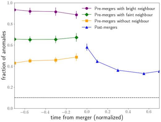
Fraction of samples outside of the training set as a function of time from merger of different types of galaxies. Pre-mergers with a bright neighbour (Fc/Fn < 2) in purple, pre-mergers with a faint neighbour (Fc/Fn > 2) in green, isolated pre-mergers in yellow and post-mergers in blue. We show the fraction of samples outside of the training set according to the threshold 2, which corresponds to 90 per cent of the training galaxies being consistent.
We now investigate other properties from the simulations that can have an effect on the anomaly score: stellar mass, redshift z, effective radius Reff, and axial ratio q. The axial ratio is derived using sextractor, and the other properties are defined by the simulations. We show in Fig. 11 how the fraction of samples inconsistent with the training set change as a function of these properties (we again choose the threshold 2 but note that the choice of the threshold does not affect the trends we observe, they only change by a scaling factor). We observe that there are more anomalous galaxies in the pre-merger stage than in the post-merger phase and that galaxies with a secondary object have, for all properties, higher fractions of anomalies. However, regardless of the galaxy being in the pre- or post-merger phase, or having or not a secondary object, the fraction of anomalies increases with increasing stellar mass and size (larger and more massive galaxies tend to be less consistent with the training set). This is not surprising, as the stellar mass distribution of the training sample does not expand to masses larger than log (M*/M⊙) = 10.75, while for the test sample we find galaxies with stellar mass up to log (M*/M⊙) = 12 (see Fig. 5). The anomaly score decreases with axial ratio (the most elongated galaxies are more anomalous). This can be explained by the absence of very elongated galaxies in our training sample. Lastly, we observe that there is not a strong correlation with redshift.
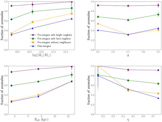
Fraction of samples outside of the training set as a function of stellar mass (top left-hand panel), redshift z (top right-hand panel), effective radius Reff (bottom left-hand panel), and axial ratio q (bottom right-hand panel). In blue we show the fraction of post-mergers, in yellow the fraction of pre-mergers without a neighbour in the image, in purple the pre-mergers with a bright neighbour and in green pre-mergers with a faint neighbour present in the image. The fractions of anomalies increase with mass and size and decreases with axial ratio, while remains constant with redshift.
One interesting fact to note here is that the distribution of test images is really being compared to the distribution of training images, and as such, by choosing a hard threshold we quantify rare objects (even in the training set) as being less consistent with the bulk of the rest of training set.
4.2 Comparison between observations and simulations
This last application focuses on investigating how we can use the anomaly detection method to compare two sets of data. Here we compare simulated data from Horizon-AGN and data from the CANDELS survey described in Section 2.2 to see if the WGAN is able to distinguish the images coming from different distributions. Assessing how well modern hydrodynamical simulations reproduce the observed properties of galaxies is a complex task because of the large number of parameters involved. The proposed approach has the advantage of collapsing all properties to one unique metric of similarity that encapsulates all morphological features.
For this application, the first thing we do is to add realistic noise to the mock observations to be able to compare the two data sets directly. We first select sky-only regions from the CANDELS-HST observation in the H-band, to create noise-only mosaics of 64 × 64 to use randomly with each galaxy from the simulations. For a given galaxy image, we then generate a corresponding Poisson noise, to which we introduced pixel-to-pixel correlation such that 1D autocorrelation power spectral density (PDS) of the sky mosaic matches the source noise. Finally, we add this correlated Poisson noise and a sky mosaic to generate mock images that match the CANDELS-HST observations.
4.2.1 Training
We train our WGAN (see Section 3.3) with a training sample composed of all the mock images from the Horizon-AGN simulation (1524 118 images), with added noise. For this application, the test set is comprised of the 17 611 CANDELS images in our sample. The stellar mass and redshift distributions for the training (Horizon-AGN) and test set (CANDELS) are shown in Fig. 12. Both sets cover the same range in stellar mass and redshift, although with a very slight difference in distribution, so any difference between the data sets is not expected to be a consequence of the selection function.
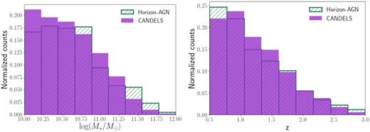
Stellar mass (left-hand panel) and redshift distribution (right-hand panel) of the training data (Horizon-AGN images, in striped green), and the test data (CANDELS images, in solid purple).
Fig. 13 shows examples of CANDELS galaxies indicating their anomaly score, the closest generated image and the residuals. As in Fig. 6, we observe that for galaxies with low anomaly score the network is able to generate a very similar image and, therefore, the residuals are low, while high anomaly scores result in high residuals (the network is not able to generate similar images). Fig. 14 shows the t-SNE reduced dimensional representation of the output of the last layer of convolutions for both the Horizon-AGN and CANDELS images. We easily observe that the two sets globally populate different parts of the space, although with some degree of overlap, which suggests that the network is able to distinguish the two populations. We investigate the reasons behind this apparent discrepancy in the following section.
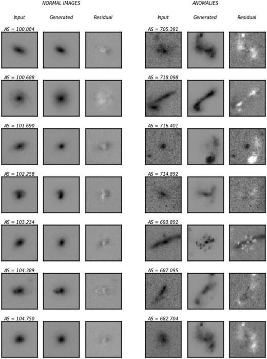
Examples of CANDELS galaxies classified as normal (left-hand panels) and anomalous (right-hand panels). Similar to Fig. 6, in the first column we show the input image, in the second column, the closest generated image, and in the third, the residual image.

t-SNE space for the output of the last convolutional layer of the trained critic. We show in green a subset of training images and in purple CANDELS images. Note the separation is much less obvious than with Fig. 7 since the distribution of images is much closer.
4.2.2 Results: Difference between Horizon-AGN and CANDELS
We compute the anomaly scores for Horizon-AGN and CANDELS images, and show their distribution in Fig. 15.
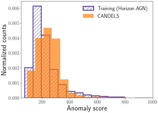
Distribution of anomaly scores for the Horizon-AGN galaxies (training sample), in striped blue, and for the CANDELS data in solid orange. The anomaly scores for the CANDELS galaxies are, overall, higher than the training set, which points at differences between the Horizon-AGN simulations and the CANDELS observations.
We observe that, even though there is considerable overlap between the two distributions, the anomaly scores for the CANDELS are, overall, higher. If the simulations were to reproduce the observed data perfectly, we would expect the distributions of the anomaly score for both the Horizon-AGN and CANDELS samples to be more consistent. However, the difference in anomaly score distribution suggests that the simulations are not able to completely reproduce the observational data from CANDELS. This could be, in part, because we did not include effects such as dust, but could also include other choices in the physical model of the simulation, or by resolution effects or other prescriptions in the radiative transfer code. Therefore this example has to be seen as an illustration of the potential of this approach to detect global subtle morphological differences between data sets coming from different origins. However, we do not aim to establish robust conclusions given the many limitations. One possible application would be exploring how different simulations, produced with different physical processes, compare with observational data. For that purpose, our WGAN could be trained on images from an observational survey, and then, anomaly scores can be computed for the observational images, and for the images from the different simulations. Comparing the distributions of anomaly scores will give information about which simulations produce images that are more consistent with the observations.
As a preliminary step forward, we show in Fig. 16 the anomaly score distribution for observed galaxies as a function of different galaxy physical properties (stellar mass, effective radius, redshift, axial ratio, Sérsic index, and morphological type). The figure reveals some interesting trends. While there is no effect on the anomaly score due to redshift, globally speaking, massive galaxies tend to be more anomalous. The smallest galaxies tend to have higher AS values, possible due to resolution effects in the simulations. Spheroidal, high Sérsic index galaxies, and point-source/compact are also skewed towards larger AS values. This suggests that compact galaxies might not be well represented in the Horizon-AGN simulation. However, this needs to be investigated further given the limitations of this comparison.

Distribution of the anomaly score for the CANDELS galaxies as a function of different properties (stellar mass, effective radius, redshift, axial ratio, Sérsic index, and morphology type). Each histogram is normalized. These plots show which properties are causing high anomaly scores. We observe that the largest and more massive galaxies tend to have higher anomaly scores, as well as spheroidal galaxies and galaxies with high Sérsic index.
5 SUMMARY
In this first proof-of-concept work, we have explored generative methods as a way to quantify anomalous objects in astronomical imaging data without labels. The method consists of, first, training a WGAN with ‘normal’ data and calculating the anomaly score of the test sample to quantify the degree of anomaly. The main advantage of such an approach is that it can learn complex representations directly from the pixel space without manual extraction of specific features. It can therefore identify subtle morphological differences and collapse morphological comparisons to one unique metric.
We have tested the method on three different applications:
In the first application we asses how accurately we can detect known differences between the training and test samples. In this case, the WGAN is trained with images of isolated galaxies (with no merger history) from the Horizon-AGN simulation, and used to identify known mergers. We show that the WGAN correctly classifies 80 per cent of the test images as anomalous with a contamination of only 10 per cent (i.e. 10 per cent of the isolated galaxies are incorrectly classified as anomalous). The percentage of anomalous images increases to 92 per cent when not considering images with very faint neighbours in the image.
In the second application we investigate how our method is able to detect anomalies caused by more subtle properties. When investigating a test sample that consist of images of merging galaxies without a visible companion in the image, we find that 45 per cent of the test set is anomalous compared to the training set. In this case, the anomaly is cause by morphological features instead of a secondary source in the image. We observe that the most anomalous objects generally have higher mass and have high axial ratio. This is because the training sample lacks galaxies with these properties. It is, therefore, useful to consider how this anomaly detection method really allows us to introspect biases in the training set as well as the physical model with which we can generate such realistic training sets.
The third application shows how the anomaly detection method can be used to compare two data sets. The training set for this example is a complete set of simulated galaxies from the Horizon-AGN simulations, and the test or comparison sample comprises observed images from the CANDELS survey. We show that the anomaly score distribution of the observations tends to peak at larger values compared to that of the simulated data. We further explore what properties were causing the main differences, to better understand how the simulations differ from the observations. We observe that the simulations were not reproducing the smallest galaxies and high Sérsic index galaxies well. This may be, in part, due to the lack of dust treatment in the radiative code, but could also be due to the resolution effects and/or other radiative processes.
The code to train our WGAN and generate is made public with this work. In future papers we plan to investigate the effect that physical processes from the simulations (such as the addition of dust) have on our analysis when comparing the Horizon-AGN simulation to the CANDELS survey. Additionally, we plan to use the WGAN anomaly detector to look for outliers in the HSC survey (Storey-Fisher et al. in preparation) and investigate its applicability in the pipelines of future surveys such as LSST and EUCLID. As part of the efforts to investigate the practical use of generative models to compare simulations to observations, we are also exploring regressive models (Zanisi et al. in preparation).
ACKNOWLEDGEMENTS
This work was supported in part by NSF (National Science Foundation) grant AST-1816330.
Footnotes
REFERENCES
APPENDIX A: TRAINING ALGORITHM
Given a batch of real and generated images, the critic is trained for ncritic iterations to approximate the Wasserstein distance, by maximizing the loss in equation (4) whilst keeping the weights of the generator fixed. Afterwards, the generator’s weight are updated for a single iteration, by maximizing equation (5), whilst the critic weights are held constant so that it minimizes the approximate Wasserstein distance. This is repeated until the network has converged. Fig. 2 shows a schematic representation the WGAN training procedure.
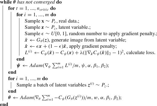
WGAN with gradient penalty training algorithm (Gulrajani et al. 2017). We use default values gradient penalty coefficient of |$\lambda\,=\,10$|, number of critic iterations per generator iteration |$n_\rm{critic}\,=\,10$|, batch size |$m\,=\,64$| and Adam hyperparameters: |$\alpha\,=\,0.00005$|, |$\beta_1=0.5$|, |$\beta_2=0.9$|.


