


ABSTRACT
Many of the planets discovered by the Kepler satellite are close orbiting super-Earths or mini-Neptunes. Such objects exhibit a wide spread of densities for similar masses. One possible explanation for this density spread is giant collisions stripping planets of their atmospheres. In this paper, we present the results from a series of smoothed particle hydrodynamics (sph) simulations of head-on collisions of planets with significant atmospheres and bare projectiles without atmospheres. Collisions between planets can have sufficient energy to remove substantial fractions of the mass from the target planet. We find the fraction of mass lost splits into two regimes – at low impact energies only the outer layers are ejected corresponding to atmosphere dominated loss, at higher energies material deeper in the potential is excavated resulting in significant core and mantle loss. Mass removal is less efficient in the atmosphere loss dominated regime compared to the core and mantle loss regime, due to the higher compressibility of atmosphere relative to core and mantle. We find roughly 20 per cent atmosphere remains at the transition between the two regimes. We find that the specific energy of this transition scales linearly with the ratio of projectile to target mass for all projectile-target mass ratios measured. The fraction of atmosphere lost is well approximated by a quadratic in terms of the ratio of specific energy and transition energy. We provide algorithms for the incorporation of our scaling law into future numerical studies.
1 INTRODUCTION
There have been a wealth of exoplanet discoveries over recent years, bringing the total number of confirmed planets to more than 4000. About 20 per cent have a mass between that of the Earth and the Neptune (henceforth super-Earth mass). Of these, two thirds orbit at a distance less than that of Mercury from their host stars, and more than three quarters are in systems with at least one other planet (NASA 2019).
Planets in this mass and orbital distance range are very diverse, with measured densities ranging from between 0.03 and 12.7 |$\mathrm{g\, cm}^{-3}$|. Even planets within the same Solar system at similar orbital radii can be vastly dissimilar. The two innermost planets of the Kepler-107 system (Bonomo et al. 2019), for example, both have similar radii (1.5–1.6R⊕), but Kepler-107b has a density of |$5.3\, \mathrm{g\, cm^{-3}}$| compared to Kepler-107c’s |$12.6\, \mathrm{g\, cm^{-3}}$|. This high density implies that Kepler-107c must have a different composition from 107b.
There are two main theories that explain the diversity of densities observed in Super-Earths and Mini-Neptunes: (1) XUV radiation from the central star (Lopez, Fortney & Miller 2012; Lopez & Fortney 2013; Owen & Wu 2013; Jin et al. 2014) strips close orbiting planets of some of their lighter elements, leaving them denser. (2) Giant impacts eject the lighter outer material (such as crust or atmosphere) from both bodies leaving a denser remnant planet (Inamdar & Schlichting 2016; Bonomo et al. 2019).
XUV radiation cannot always explain large differences in density for planets orbiting at similar semimajor axes in the same planetary system, for example, Kepler-107b and c. These two planets orbit at a similar distance from their parent star and have similar physical radii but differ significantly in planetary mass. The outer Kepler-107c is more than twice as dense as the innermost 107b. Kepler-107c’s density can not be explained by XUV radiation because it is orbiting outside the less massive and also less dense Kepler-107b, which would have lost more material due to irradiation. Thus, a giant impact is the best explanation (Bonomo et al. 2019).
Giant impacts have been suggested as the explanation for density diversity in several planetary systems (Liu et al. 2015; Inamdar & Schlichting 2016). In addition, many of the tightly orbiting high-multiplicity systems detected by Kepler appear to be on the borders of stability (Fang & Margot 2013). Therefore, it is not unreasonable to consider the planets g⊕tationally interacting with one another in such a way that either they eject one or both planets or that they collide with one another. Barnes & Raymond (2004) showed that small perturbations in orbit will lead to such ejections or collisions. Volk & Gladman (2015) even suggested close orbiting groups of planets are common in the formation of inner solar systems (a < 0.5 au), including our own, but that they are not stable long term, and will undergo collisional disruption and consolidation. This suggests that the high multiplicity systems that we observe are either these initial unstable systems, or that the planets are in an arrangement that is stable for long time periods.
Several previous works (e.g. Schlichting, Sari & Yalinewich 2015; Inamdar & Schlichting 2016) have demonstrated that giant impacts have the potential to remove large fractions of these planets’ atmospheres, leading to substantial density enhancement. In this paper, we directly calculate atmosphere stripping via 3D modelling of head-on giant impacts between Mini-Neptune mass planets with significant atmospheres and lower mass bare super-Earth impactors.
1.1 Previous work
Until recently, simulations of atmospheric losses due to such giant collisions were too computationally expensive to run within a reasonable time frame. Recent advances, however, have meant high resolutions are now much more attainable.
Because of computational demands much early work focused on analytical predictions (some of which focus on significantly lower mass atmospheres than we consider here, such as Earth-like atmospheres), for example, Genda & Abe (2003) who discuss how much of an Earth-like protoplanet’s atmosphere is likely to survive the giant impact phase. They used one-dimensional models to calculate the amount of material jettisoned after a collision from the ground velocity beneath it, showing that for the canonical Moon-forming impact only ≈20 per cent of mass would be lost. Genda & Abe (2003) also showed that the ground velocity needs to reach the escape velocity for total atmosphere erosion. Schlichting et al. (2015) expanded upon this by formulating a method of predicting atmospheric loss from a wide range of projectiles colliding with terrestrial planets. This method is the one used by Inamdar & Schlichting (2016) when discussing the density diversity of super-Earth mass exoplanets. Inamdar & Schlichting (2016) showed that a single collision between similarly sized exoplanets can cause a decrease in the mass ratio of atmospheric envelope to central core material by a factor of 2, which in turn leads to a density increase of a factor of 2–3. Inamdar & Schlichting (2016) thus suggested giant impacts as a cause for the observed density diversity.
Despite computational limitations some progress has been made in simulating collisions of planets with gaseous envelopes. Liu et al. (2015) considered a model of the Kepler-36 system (with target planets of 6–8 per cent atmosphere by mass). They found that a collision could cause the density difference observed between the two planets in this system, and suggested that giant collisions might therefore be the cause of the dispersion we observe in the mass–radius relationship for super-Earth mass planets. Hwang et al. (2017a,b) used an N-body code to model the evolution and stability of high multiplicity planetary systems (specifically Kepler-11 and Kepler-36). For the collisions, they used a smoothed particle hydrodynamics (sph) code and assumed atmosphere mass fractions of 5–15 per cent to determine the results of highly grazing collisions (collisions where only the atmospheres overlap), they showed that typically the higher mass core will accrete more of the disrupted gas envelope leading to increasing density contrasts between the two planets. Due to problems with their equation of state, however, they where unable to simulate the results of head-on collisions. Kegerreis et al. (2018) also used sph to model collisions involving targets with atmospheres, to see if they could model the formation of Uranus’ off-axis rotation and unusual magnetic field. Unlike this paper, Kegerreis et al. (2018) focus mostly on higher impact parameter collisions in order to study the change in rotation. They considered ice giants as opposed to the metal and silicate planets with atmospheres studied in this work.
In this paper, we present the results from a series of head-on collisions between super-Earth mass planets where each of the three different mass targets is a Mini-Neptune with a significant hydrogen envelope (8–33 per cent). We run a large series of numerical simulations with a wide array of atmosphere-less super-Earth projectiles. We provide scaling relations for material loss applicable to a wide range of masses that can be used in N-body simulations and population synthesis models.
2 METHODS
2.1 Numerical code
The simulations presented in this paper were run using the sph code gadget-2 (Springel 2005). Although gadget-2 was initially designed for simulations on cosmological scales, we have used a modified version to model our planets that includes tabulated equations of state (EOS) for the planetary constituents. For further detail on these modifications see Marcus et al. (2009) and Ćuk & Stewart (2012). We further modified gadget-2 to include an ideal gas atmosphere component.
In sph codes, such as gadget-2, the material is split into separate particles each representing an ensemble of material. The continuous fluid properties, such as the density, for each ensemble of particles are calculated using kernel interpolation methods. The g⊕tational forces on the other hand are calculated using hierarchical tree methods (Springel 2005). We ran gadget-2 in ‘Newtonian’ mode with time-step synchronization, and the standard relative cell-opening criterion. We use the standard time-step criterion as described in Springel (2005), where the smaller of the time-step based on the g⊕tational softening and the acceleration, or the courant condition is used (with a courant factor of 0.1). We use the standard artificial viscosity formulation for gadget-2 as described in Springel (2005), with a strength parameter of 0.8.
We modelled the planets as two or three material systems, each planet (both projectile and target) consisting of iron core, forsterite (silicate) mantle, and a hydrogen atmosphere for the target only. In a similar fashion to prior studies (Marcus et al. 2009; Ćuk & Stewart 2012), the mantle was twice the mass of core. We modelled the atmosphere as a monatomic ideal gas for simplicity and ease of comparison (see Section 4.1). Tabulated ANEOS/MANEOS EOS from Melosh (2007) were used for the iron and forsterite (these tables are available from Carter, Lock & Stewart 2019).
2.2 Hardware
The simulations were each run using a full node on the University of Bristol’s Bluecrystal supercomputers, either on phase 3 or phase 4. Phase 3 nodes consist of 16 core 2.6 GHz SandyBridge processors with 59.7 GiB RAM altogether (Gardiner 2015), whilst phase 4 nodes have two 14 core 2.4 GHz Intel E5-2680 v4 (Broadwell) CPUs with the whole node having a combined 128 GiB of RAM (Gardiner 2017). Each collision took between half a day and a day depending on the masses and impact energies involved.
2.3 Initial conditions
To generate the initial planets, we began by creating the central core and mantle. To generate density profiles we used radial temperature profiles (from Valencia, O’Connell & Sasselov 2006) as well as estimates for the average bulk density of each type of material (i.e core or mantle) and the radial range that the core and mantle occupies. From this initial assumption of constant density per material layer, we iteratively generated new density profiles using g⊕tational and hydrostatic pressure calculations, until we obtained a density profile that was consistent with our EOS, the expected hydrostatic pressure, and the input temperature profile.
Once a consistent profile was obtained, it was then used to generate the position of each of the particles by splitting the planet into a number of radial bins based on its mass and randomly positioning a number of particles within each bin proportional to the bin’s mass. The final number of bins being adjusted so that we could reach our desired mass to a tolerance of 1 per cent. The type of material being added to each bin was decided by the material ranges given for the initial density profile. After generating an initial sph planet it was then equilibrated in isolation for 105 s (simulated seconds) using a preliminary run of gadget-2, to ensure that we were running simulations with a planet that was stable. During equilibration we used two ‘artificial cooling’ methods, velocity damping of the particles, i.e applying a restitution factor of 50 per cent each time-step (see Carter et al. 2018), and also entropy forcing, the entropy of each particle is reset to a constant value for each material at every time-step (|$1.3\, \mathrm{kJ\, K^{-1}\, kg^{-1}}$| for the iron core, |$3.2\, \mathrm{kJ\, K^{-1}\, kg^{-1}}$| for the mantle). This entropy forcing ensures that we produce planets with isentropic layers.
We then used this radial mass profile for the atmosphere to determine the position of atmosphere particles, by splitting the profile into radial bins and placing particles proportionally to the mass of the bins at random positions within them, in a similar fashion to the core and mantle. This new body was equilibrated for a longer time of 4–8|$\times 10^5\, \mathrm{s}$| until the radius of the planet had converged to a constant value. The pseudo-entropy of the atmosphere was forced to a value of |$5\times 10^{11}\, \mathrm{Ba\, g^{-\gamma }\, cm^{3\gamma }}$| where the adiabatic index was γ = 5/3, this ensured that the atmosphere would not reach densities where it would sink underneath the mantle and core material, but also that the base of the ideal gas atmosphere was as close as possible to our predicted temperatures.
For the core and mantle of our targets, we used a resolution of 105 particles. All other particles in each simulation were made the same mass as the core and mantle particles, resulting in a total resolution between 1.2 × 10⁵ and 2.5 × 10⁵ particles. This results in an atmosphere ‘thickness’ of between 5 and 10 layers of particles. Our total particle number is smaller than that suggested by Kegerreis et al. (2019), however, we are interested in large changes in mass of the largest remnant so our resolution should be sufficient. We have run resolution tests of head-on collisions of 5 M⊕ planets with 0.9 M⊕ atmospheres against one another at both half and double our standard resolution (of 105 particles in the target core and mantle) at impact velocities of 20 and 40 |$\mathrm{km\, s^{-1}}$|. The key quantities we measure are mass of the largest remnant, atmosphere loss fraction, and core and mantle loss fraction, each vary from the mean value at that velocity by less than 5 per cent except for the core and mantle loss fraction at low velocity, where only a very small number of particles are being lost. We did not consider losses or remnants of only a few hundred particles resolvable with sph methods.
2.3.1 The point of impact
In collisional studies, impact parameters such as velocity, impact energy, etc. are normally measured in terms of the point of first physical contact between the two planetary bodies (e.g. Leinhardt & Stewart 2012). For planets with atmospheres this becomes more complex, however, as atmosphere densities decay approximately exponentially so there is no clear boundary at which the atmosphere ends. Tidal forces between planets also have a stronger distorting effect on the atmosphere than the core and mantle. Thus, we use the time when mantle surfaces touched as our point of impact because this can be clearly defined.
To obtain an initial start position from our desired collision parameters (for example, velocity and impact angle), the following process was used: (1) the two planets were represented by point masses at their centres, and these two planets were placed at their position at the point of impact and set at the predicted velocity; 2) Time reversal symmetry was then used to trace the path of the projectile back to a separation of five times the sum of the projectile and target mantle radii (excluding atmosphere). To determine the projectiles path we used a simple Verlet integrator, set the target planet to be centred on the origin, and calculated the acceleration as given by the relative g⊕tational force between two-point particles. The choice of starting separation was a somewhat arbitrary one intended to reduce the tidal forces compared to the starting distances of previous similar studies due to us equilibrating planets in isolation and atmospheres being more easy to tidally distort.
Note using the point where mantles touch as our point of impact is not without its drawbacks. As can be observed in Fig. 1, the presence of the atmosphere causes a significant observable slowing of the relative impact velocity. This slowing is due to atmospheric drag that distorts the projectile planet. For some collisions, this distortion is even present when the leading edge of the projectile is greater than an atmospheric scale height from the target. In further calculations, which use impact energy, we used the measured velocity instead of the predicted input value. To measure this collision point precisely, we re-simulated the point of impact for our collisions with a higher output frequency (snapshots were taken every 3 s as opposed to every 100).
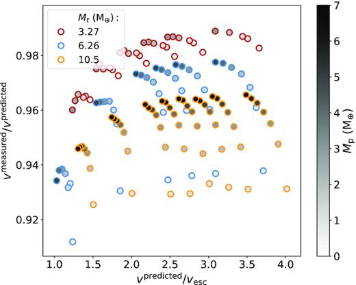
Comparisons of the predicted velocity for the three targets and the ratio between measured and predicted impact velocities. Impact velocities are given in terms of the mutual escape velocity (|$v_{\mathrm{esc}}=(2GM_{\mathrm{tot}}/R^{^{\prime }})^{\frac{1}{2}}$| where |$R^{^{\prime }}=\left(3M_{\mathrm{tot}}/4\pi \rho _{\mathrm{bulk}}\right)^{\frac{1}{3}}$| and ρbulk is the bulk density of the simulated target). Edge colours show target mass, while central colours show projectile mass. The reduced velocity compared to the prediction can be considered a measure of the drag caused by the atmosphere. As might be expected, the denser, higher mass atmospheres around the larger targets tend to cause more drag, the lower mass and lower velocity projectiles tend to experience proportionally more drag as well due to their lower momenta.
2.3.2 Input parameters
Simulation parameters and results for head-on collisions between a |$6.26\, \mathrm{M}_{\oplus }$| target, with a mantle surface radius of |$1.49\, \mathrm{R}_{\oplus }$|, and an atmosphere scale height of |$0.60\, \mathrm{R}_{\oplus }$|, and a projectile of mass Mp and radius Rp. The first digit of the collision ID denotes the non-atmospheric target mass (|$M_\mathrm{t}^{\mathrm{core}} = 5.01 \, \mathrm{M}_{\oplus }$| therefore |$M_\mathrm{t}^{\mathrm{atmos}} = 1.25 \, \mathrm{M}_{\oplus }$|). vinit is the initial relative speed of the projectile with respect to the target, at an initial separation of S to give a predicted impact speed of |$v_{\mathrm{imp}}^{\mathrm{pred}}$|, the measured velocity at the point where the mantles touch is |$v_{\mathrm{imp}}^{\mathrm{meas}}$|. MLR is the total mass of the largest post-collision remnant, where |$M_{\mathrm{LR}}^{\mathrm{atmos}}$| and |$M_{\mathrm{LR}}^{\mathrm{core}}$| are the atmospheric and non-atmospheric masses, respectively, the final column gives the category we have given that collision. We have used ‘-’ to denote final snapshots where there where too few particles in the largest remnant to be able to properly resolve. Simulation data for |$M_\mathrm{t} = 3.27 \, \mathrm{M}_{\oplus }$| and |$M_\mathrm{t} = 10.5 \, \mathrm{M}_{\oplus }$| can be found in Tables A1 and A2.
| ID | Mp | Rp | |$v_{\mathrm{imp}}^{\mathrm{pred}}$| | |$\frac{v_{\mathrm{imp}}^{\mathrm{pred}}}{v_{\mathrm{esc}}}$| | |$v_{\mathrm{imp}}^{\mathrm{meas}}$| | |$\frac{v_{\mathrm{imp}}^{\mathrm{meas}}}{v_{\mathrm{esc}}}$| | vinit | |$\frac{v_{\mathrm{init}}}{v_{\mathrm{esc}}}$| | S | MLR | |$M_{\mathrm{LR}}^{\mathrm{atmos}}$| | |$M_{\mathrm{LR}}^{\mathrm{core}}$| | |$\frac{M_{LR}}{M_{\mathrm{tot}}}$| | |$X_{\mathrm{loss}}^{\mathrm{atmos}}$| | |$X_{\mathrm{loss}}^{\mathrm{c\&m}}$| | Category |
|---|---|---|---|---|---|---|---|---|---|---|---|---|---|---|---|---|
| M⊕ | R⊕ | |$\mathrm{km}\, \mathrm{s}^{-1}$| | |$\mathrm{km}\, \mathrm{s}^{-1}$| | |$\mathrm{km}\, \mathrm{s}^{-1}$| | R⊕ | M⊕ | M⊕ | M⊕ | ||||||||
| 5–0 | 0.25 | 0.62 | 20.00 | 1.24 | 18.24 | 1.13 | 9.38 | 0.58 | 11.15 | 6.50 | 1.24 | 5.26 | 1.0 | 0.01 | −0.0 | AM-CM |
| 5–1 | 0.25 | 0.62 | 30.00 | 1.85 | 27.92 | 1.73 | 24.25 | 1.50 | 11.16 | 6.43 | 1.17 | 5.26 | 0.99 | 0.06 | −0.0 | AL-CM |
| 5–2 | 0.25 | 0.62 | 40.00 | 2.47 | 37.38 | 2.31 | 35.89 | 2.22 | 11.15 | 6.30 | 1.05 | 5.26 | 0.97 | 0.16 | −0.0 | AL-CM |
| 5–3 | 0.25 | 0.62 | 45.00 | 2.78 | 42.12 | 2.60 | 41.39 | 2.56 | 11.18 | 6.22 | 0.97 | 5.25 | 0.96 | 0.22 | 0.0 | AL-CM |
| 5–4 | 0.25 | 0.62 | 50.00 | 3.09 | 46.84 | 2.90 | 46.77 | 2.89 | 11.15 | 6.14 | 0.89 | 5.25 | 0.94 | 0.29 | 0.0 | AL-CM |
| 5–5 | 0.25 | 0.62 | 60.00 | 3.71 | 56.27 | 3.48 | 57.34 | 3.54 | 11.18 | 5.94 | 0.71 | 5.23 | 0.91 | 0.43 | 0.01 | AL-CM |
| 5–6 | 0.75 | 0.88 | 20.00 | 1.21 | 18.66 | 1.13 | 10.22 | 0.62 | 11.93 | 6.90 | 1.13 | 5.76 | 0.98 | 0.1 | 0.0 | AL-CM |
| 5–7 | 0.75 | 0.88 | 30.00 | 1.81 | 28.65 | 1.73 | 24.58 | 1.48 | 11.93 | 6.66 | 0.91 | 5.75 | 0.95 | 0.27 | 0.0 | AL-CM |
| 5–8 | 0.75 | 0.88 | 40.00 | 2.41 | 38.37 | 2.31 | 36.11 | 2.18 | 11.96 | 6.29 | 0.56 | 5.73 | 0.9 | 0.55 | 0.01 | AL-CM |
| 5–9 | 0.75 | 0.88 | 45.00 | 2.71 | 43.20 | 2.61 | 41.58 | 2.51 | 11.94 | 6.11 | 0.41 | 5.69 | 0.87 | 0.67 | 0.01 | AL-CM |
| 5–10 | 0.75 | 0.88 | 60.00 | 3.62 | 57.66 | 3.48 | 57.48 | 3.47 | 11.96 | 4.62 | 0.07 | 4.55 | 0.66 | 0.94 | 0.21 | AL-CE |
| 5–11 | 1.25 | 1.02 | 20.00 | 1.18 | 18.63 | 1.10 | 10.11 | 0.60 | 12.35 | 7.28 | 1.02 | 6.26 | 0.97 | 0.18 | 0.0 | AL-CM |
| 5–12 | 1.25 | 1.02 | 30.00 | 1.77 | 28.80 | 1.70 | 24.54 | 1.45 | 12.35 | 6.92 | 0.68 | 6.25 | 0.92 | 0.46 | 0.0 | AL-CM |
| 5–13 | 1.25 | 1.02 | 45.00 | 2.65 | 43.52 | 2.57 | 41.56 | 2.45 | 12.37 | 5.86 | 0.19 | 5.68 | 0.78 | 0.85 | 0.09 | AL-CA |
| 5–14 | 1.25 | 1.02 | 50.00 | 2.95 | 48.37 | 2.85 | 46.93 | 2.77 | 12.36 | 5.04 | 0.09 | 4.95 | 0.67 | 0.93 | 0.21 | AL-CE |
| 5–15 | 1.25 | 1.02 | 60.00 | 3.54 | 58.10 | 3.42 | 57.46 | 3.39 | 12.36 | 2.94 | 0.00 | 2.94 | 0.39 | 1.0 | 0.53 | TAL-CE |
| 5–16 | 2.00 | 1.18 | 20.00 | 1.14 | 18.74 | 1.07 | 9.66 | 0.55 | 12.81 | 7.89 | 0.91 | 6.99 | 0.95 | 0.27 | 0.0 | AL-CM |
| 5–17 | 2.00 | 1.18 | 30.00 | 1.71 | 28.90 | 1.65 | 24.36 | 1.39 | 12.82 | 7.49 | 0.53 | 6.96 | 0.91 | 0.58 | 0.01 | AL-CM |
| 5–18 | 2.00 | 1.18 | 40.00 | 2.28 | 38.81 | 2.22 | 35.96 | 2.05 | 12.83 | 6.42 | 0.21 | 6.22 | 0.78 | 0.83 | 0.11 | AL-CA |
| 5–19 | 2.00 | 1.18 | 45.00 | 2.57 | 43.72 | 2.50 | 41.45 | 2.37 | 12.81 | 5.48 | 0.09 | 5.38 | 0.66 | 0.93 | 0.23 | AL-CA |
| 5–20 | 2.00 | 1.18 | 50.00 | 2.85 | 48.63 | 2.78 | 46.83 | 2.67 | 12.84 | 4.15 | 0.01 | 4.14 | 0.5 | 0.99 | 0.41 | TAL-CE |
| 5–21 | 2.00 | 1.18 | 60.00 | 3.43 | 58.40 | 3.33 | 57.39 | 3.28 | 12.83 | 1.12 | 0.00 | 1.12 | 0.14 | 1.0 | 0.84 | TAL-CE |
| 5–22 | 3.01 | 1.32 | 20.00 | 1.10 | 18.77 | 1.03 | 8.69 | 0.48 | 13.24 | 8.73 | 0.81 | 7.92 | 0.94 | 0.35 | 0.01 | AL-CM |
| 5–23 | 3.01 | 1.32 | 30.00 | 1.65 | 28.89 | 1.59 | 23.99 | 1.32 | 13.25 | 8.38 | 0.49 | 7.89 | 0.9 | 0.61 | 0.02 | AL-CM |
| 5–24 | 3.01 | 1.32 | 40.00 | 2.20 | 38.88 | 2.14 | 35.71 | 1.96 | 13.25 | 6.76 | 0.17 | 6.59 | 0.73 | 0.86 | 0.18 | AL-CA |
| 5–25 | 3.01 | 1.32 | 45.00 | 2.47 | 43.82 | 2.41 | 41.24 | 2.27 | 13.25 | 5.45 | 0.07 | 5.39 | 0.59 | 0.94 | 0.33 | AL-CA |
| 5–26 | 3.01 | 1.32 | 50.00 | 2.75 | 48.74 | 2.68 | 46.64 | 2.56 | 13.26 | 3.78 | 0.00 | 3.78 | 0.41 | 1.0 | 0.53 | TAL-CE |
| 5–27 | 3.01 | 1.32 | 60.00 | 3.30 | 58.54 | 3.22 | 57.23 | 3.15 | 13.28 | – | – | – | – | 1.0 | – | SCD |
| 5–28 | 4.01 | 1.43 | 20.00 | 1.06 | 18.76 | 1.00 | 7.47 | 0.40 | 13.58 | 9.66 | 0.81 | 8.85 | 0.94 | 0.35 | 0.02 | AL-CM |
| 5–29 | 4.01 | 1.43 | 30.00 | 1.59 | 28.89 | 1.53 | 23.57 | 1.25 | 13.60 | 9.37 | 0.51 | 8.86 | 0.91 | 0.59 | 0.02 | AL-CM |
| 5–30 | 4.01 | 1.43 | 40.00 | 2.12 | 38.91 | 2.07 | 35.43 | 1.88 | 13.60 | 7.46 | 0.17 | 7.29 | 0.73 | 0.86 | 0.19 | AL-CA |
| 5–31 | 4.01 | 1.43 | 45.00 | 2.39 | 43.87 | 2.33 | 41.00 | 2.18 | 13.59 | 5.95 | 0.06 | 5.89 | 0.58 | 0.95 | 0.35 | TAL-CA |
| 5–32 | 4.01 | 1.43 | 50.00 | 2.66 | 48.80 | 2.59 | 46.43 | 2.47 | 13.60 | 4.05 | 0.00 | 4.05 | 0.39 | 1.0 | 0.55 | TAL-CE |
| 5–33 | 4.01 | 1.43 | 60.00 | 3.19 | 58.63 | 3.11 | 57.06 | 3.03 | 13.59 | 0.30 | 0.00 | 0.30 | 0.03 | 1.0 | 0.97 | SCD |
| 5–34 | 5.01 | 1.52 | 20.00 | 1.03 | 18.68 | 0.96 | 5.80 | 0.30 | 13.84 | 10.72 | 0.79 | 9.93 | 0.95 | 0.37 | 0.01 | AL-CM |
| 5–35 | 5.01 | 1.52 | 30.00 | 1.54 | 28.88 | 1.49 | 23.10 | 1.19 | 13.85 | 10.38 | 0.53 | 9.85 | 0.92 | 0.58 | 0.02 | AL-CM |
| 5–36 | 5.01 | 1.52 | 40.00 | 2.06 | 38.93 | 2.00 | 35.12 | 1.81 | 13.84 | 8.34 | 0.20 | 8.14 | 0.74 | 0.84 | 0.19 | AL-CA |
| 5–37 | 5.01 | 1.52 | 45.00 | 2.32 | 43.89 | 2.26 | 40.73 | 2.10 | 13.85 | 6.93 | 0.08 | 6.85 | 0.62 | 0.94 | 0.32 | AL-CA |
| 5–38 | 5.01 | 1.52 | 50.00 | 2.57 | 48.83 | 2.51 | 46.19 | 2.38 | 13.86 | 4.80 | 0.00 | 4.80 | 0.43 | 1.0 | 0.52 | TAL-CE |
| 5–39 | 5.01 | 1.52 | 60.00 | 3.09 | 58.65 | 3.02 | 56.86 | 2.93 | 13.88 | 0.93 | 0.00 | 0.93 | 0.08 | 1.0 | 0.91 | SCD |
2.4 Run parameters
2.5 Analysis methods
2.5.1 Determining bound material
To determine what material was bound in the largest post-collision remnant we used the same iterative method as Marcus et al. (2009) and Carter et al. (2018). We began by locating the particle closest to the potential minimum and using kinetic energy and g⊕tational potential to determine which other particles were g⊕tationally bound to this deepest particle. Using the total mass and centre of mass of these particles as our new seed, we then iteratively ran through the process of determining that extra particles were bound to the seed, and then adding them to the seed, until either the change in mass of the seed was below a set tolerance or a maximum number of iterations had been reached. For our simulations we, obtained single particle differences in mass within a few iterations so our tolerance was set to a single particles mass, and the maximum number of iterations was never reached. Material type was also tracked to determine the mass of each type of material, which was unbound or part of the largest remnant.
2.5.2 Collision categorization
To categorize the collision outcomes for our data, we consider separately atmosphere (A) and core and mantle material (C). For atmospheres if there was greater than 95 per cent of the initial atmosphere mass in the final remnant we considered there to be a merger (AM), on the other hand if there was less than 5 per cent remaining we categorized this as total loss (TAL), the rest were considered to undergo partial loss (AL). Although hydrogen atmospheres as small as |$0.1\small{--}1{{\ \rm per\ cent}}$| of a planet’s total mass can have a significant effect on its radius, we do not have the resolution to accurately probe atmosphere mass-losses that small. For core and mantle, we define mergers (CM) for >95 per cent of the total mass of core and mantle from both projectile and target remaining in the largest remnant. If the mass of core and mantle in the largest remnant is greater than that initially in the target we have an accretion event (CA), if it is less we have an erosion event (CE). If there was less than 10 per cent of the total mass remaining in the largest remnant we define it as a supercatastrophic disruption (SCD). Tables 1, A1, and A2 categorize our final results for each collision using this system.
3 RESULTS
The main aim of this paper is to determine scaling laws for atmosphere loss as well as total material loss during head-on giant impacts. The wide breadth of impact energies that are simulated in this work have uncovered a broad range of outcomes from near perfect merging events to highly energetic catastrophic disruption (see Fig. 2).
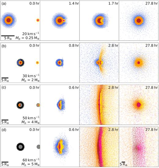
Cross-sectional snapshots sliced through the mid-plane for a series of head-on collisions showing different collision outcomes from merging to catastrophic disruption as the specific relative kinetic energy QR increases from row A to row D. Colour denotes material, red and pink – iron core, orange and yellow – forsterite mantle, and blue – hydrogen atmosphere. The additional colours in the first panel denote material that will not be bound by the end of the simulation, black being atmosphere, and grey core or mantle. All collisions shown have the same target mass (|$M_\mathrm{t} = 6.26\, \mathrm{M}_{\oplus }$|) but differ in projectile mass (Mp) and impact speed (|$\mathbf {v_\mathrm{imp}}$|): (a) Atmosphere and core and mantle merger – |$\mathbf {v_\mathrm{i}} = 20$| km s−1, |$M_\mathrm{p}=0.25\, \mathrm{M}_{\oplus }$| (Table 1, 5–0); (b) Atmosphere loss and core and mantle merger – |$\mathbf {v_\mathrm{i}} = 30$| km s−1, |$M_{\mathrm{p}}=2\, \mathrm{M}_{\oplus }$| (Table 1, 5–17); (c) Total atmosphere loss and core and mantle erosion – |$\mathbf {v_\mathrm{i}} = 50$| km s−1, |$M_\mathrm{p}=4\, \mathrm{M}_{\oplus }$| (Table 1, 5–32); (d) Supercatastrophic disruption |$\mathbf {v_\mathrm{i}} = 60$| km s−1, |$M_\mathrm{p}=5\, \mathrm{M}_{\oplus }$| (Table 1, 5–39). Post-collision remnants were inflated in comparison to the initial planets and the expected radius of the resultant planet. This ‘puffiness’ is because we do not cool our final remnants until they reach equilibrium, we only run the simulations until the mass of bound material converges. Videos of these four collisions can be found online at http://www.star.bris.ac.uk/TDenman/Paper1_Videos/.
In the process of determining the loss scaling laws we have found that the atmosphere loss, core and mantle material loss, and the largest remnant mass are well-behaved functions of specific impact energy: |$Q_\mathrm{R} = \frac{1}{2}\mu V_{\mathrm{imp}}^2 / M_\mathrm{tot}$|, where μ is the reduced mass, Vimp is the impact velocity, and Mtot is the sum of the projectile and target masses (see Leinhardt & Stewart 2012). We find that atmosphere dominates the material lost until the impact energy is large enough to remove more than 80 per cent of the atmosphere at which point mantle and core material begin to be removed significantly as well. It is also at this point that there is a break and steepening in slope of the largest post collision remnant mass (MLR) as a function of QR (Fig. 4). In other words, the atmosphere of the target planet cannot be completely removed in one giant impact without significantly eroding the planet.
3.1 Mass-loss
Fig. 3 shows the largest remnant mass from our simulations as a function of specific impact energy for collisions with a target of mass |$M_\mathrm{t}=10.5\, \mathrm{M}_{\oplus }$|. Each different colour represents a different projectile mass (Mp). Instead of a straight line (as in Leinhardt & Stewart 2012), our results appear to show two separate linear regimes: a shallower low-energy one and a steeper high-energy one.
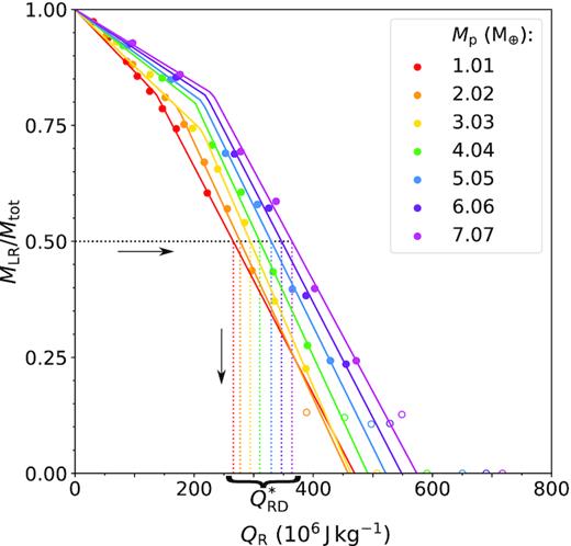
A comparison of the mass of the largest remnant for each collision compared with its specific impact energy, overlaid with a graphical representation of the process used to determine |$Q_{\mathrm{RD}}^*$|. The circles represent the fraction of the total mass which remains in the largest remnant after a collision with a target mass of |$M_\mathrm{t} = 10.5 \, \mathrm{M}_{\oplus }$| as a function of specific impact energy QR. Each colour indicates one of seven Mp values. A filled circle represents a point used for fits, whilst the open circles are points with |$\frac{M_{\mathrm{LR}}}{M_{\mathrm{tot}}}\lt 0.2$| that we considered too close to the supercatastrophic disruption regime, which our fit is not designed to cover, for all collisions where <100 particles were observed in the largest remnant, we also considered the results to be below the resolution limit of the simulation. The solid lines represent our fit to the data for each projectile-target mass ratio, following equation (8). From this fit, the empirically determined value of |$Q_{\mathrm{RD}}^*$| is shown on the horizontal axis by the intersection of a coloured dotted line matching the Mp colour and MLR/Mtot = 0.5 on the y-axis.
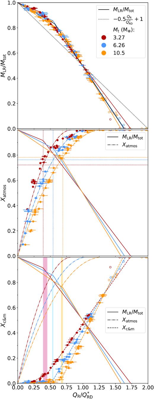
Top: MLR versus |$Q_\mathrm{R}/Q_{\mathrm{RD}}^*$| for all simulations. Colour indicates target mass, the open circles represent points that were excluded from the fit. Coloured solid lines are best fits to data for a given Mt. The black solid line is the best fit to the entire data set. The dotted black line is the universal law from Leinhardt & Stewart (2012). Middle: Fraction of atmosphere lost versus |$Q_\mathrm{R}/Q_{\mathrm{RD}}^*$|. The dashed coloured lines indicate best fits. The dotted vertical and horizontal lines show the specific energy of the break in the MLR fit and the respective fraction of atmosphere loss. Bottom: Fraction of core and mantle lost versus |$Q_\mathrm{R}/Q_{\mathrm{RD}}^*$|. The dashed lines are a broken linear fit. The shaded vertical sections show the difference between the specific energy of the break in the MLR fit and the break in the core loss fit. For all three graphs, the horizontal error bars represent the error in the |$Q_{\mathrm{RD}}^*$| determination method.
To ensure a robust fitting method, despite the low number of data points, we began by generating multiple random sets of input parameters for least-squares fitting. We determined a best fitting set of output parameters for each input set, and chose the fit with the smallest squared residuals as our final best fit. The fits we obtain for each set of projectile and target masses can then be used to determine the catastrophic disruption threshold by measuring the energy at which half the mass of the system is in the largest remnant (as shown in Fig. 3). The errors on |$Q_{\mathrm{RD}}^*$| were determined by propagating errors generated by the least-squares fitting algorithm.
Parameters for fits using equation (10) to the largest remnant mass with |$Q_{\mathrm{RD}}^*$| normalized specific impact energy.
| Mt (M⊕) | m|$_{\mathrm{2}}^{\mathrm{LR}}$| | cLR | Qpiv/Q|$_{\mathrm{RD}}^{*}$| |
|---|---|---|---|
| 3.27 | −0.68 ± 0.01 | 0.92 ± 0.01 | 0.39 ± 0.01 |
| 6.26 | −0.78 ± 0.02 | 0.86 ± 0.01 | 0.54 ± 0.02 |
| 10.5 | −0.85 ± 0.02 | 0.76 ± 0.01 | 0.69 ± 0.02 |
| Mt (M⊕) | m|$_{\mathrm{2}}^{\mathrm{LR}}$| | cLR | Qpiv/Q|$_{\mathrm{RD}}^{*}$| |
|---|---|---|---|
| 3.27 | −0.68 ± 0.01 | 0.92 ± 0.01 | 0.39 ± 0.01 |
| 6.26 | −0.78 ± 0.02 | 0.86 ± 0.01 | 0.54 ± 0.02 |
| 10.5 | −0.85 ± 0.02 | 0.76 ± 0.01 | 0.69 ± 0.02 |
Parameters for fits to the fraction of atmosphere lost from the largest remnant with |$Q_{\mathrm{RD}}^*$| normalized specific energy using equation (11).
| Target mass (M⊕) | A |
|---|---|
| 3.27 | 2.42 ± 0.06 |
| 6.26 | 1.89 ± 0.03 |
| 10.5 | 1.54 ± 0.02 |
| Target mass (M⊕) | A |
|---|---|
| 3.27 | 2.42 ± 0.06 |
| 6.26 | 1.89 ± 0.03 |
| 10.5 | 1.54 ± 0.02 |
We also investigate the dependence of core and mantle loss on the impact energy (bottom panel Fig. 4). We observe a similar broken linear relation to the broken linear relation seen for the mass of the largest remnant (Figs 3 and 4, top). In this case, we have a shallow gradient below the pivot energy (negligible for the two larger mass targets) indicating very little core and mantle mass-loss, and a much steeper gradient (therefore much greater loss) above. For lower mass targets (lower atmosphere fractions), there is greater loss of core and mantle at low energies.
Parameters for these fits are given in Table 4. As can be seen from the coloured vertical bars in the bottom panel of Fig. 4, there appears to be a correlation between this pivot energy and the pivot energy found for the mass of the largest remnant. The similar energies of these pivot points implies that the break in slope for largest remnant mass is due to the break in slope for loss of core and mantle material. We therefore categorize impacts into two energy loss regimes: below the pivot energy we have atmosphere-dominated loss, and above it we have substantial core and mantle loss.
Parameters for fits using equation (12) to the fraction of core material lost from the largest remnant with |$Q_{\mathrm{RD}}^*$| normalized specific energy.
| Mt (M⊕) | m1 | m2 | c|$^{\mathrm{c\&m}}$| | Qpiv/Q|$_{\mathrm{RD}}^{*}$| |
|---|---|---|---|---|
| 3.27 | 0.28 ± 0.02 | 0.73 ± 0.01 | 0.08 ± 0.01 | 0.45 ± 0.01 |
| 6.26 | 0.03 ± 0.03 | 0.88 ± 0.02 | 0.02 ± 0.01 | 0.53 ± 0.01 |
| 10.5 | 0.07 ± 0.03 | 1.02 ± 0.02 | 0.03 ± 0.01 | 0.67 ± 0.01 |
| Mt (M⊕) | m1 | m2 | c|$^{\mathrm{c\&m}}$| | Qpiv/Q|$_{\mathrm{RD}}^{*}$| |
|---|---|---|---|---|
| 3.27 | 0.28 ± 0.02 | 0.73 ± 0.01 | 0.08 ± 0.01 | 0.45 ± 0.01 |
| 6.26 | 0.03 ± 0.03 | 0.88 ± 0.02 | 0.02 ± 0.01 | 0.53 ± 0.01 |
| 10.5 | 0.07 ± 0.03 | 1.02 ± 0.02 | 0.03 ± 0.01 | 0.67 ± 0.01 |
An important point to note here is that at this pivot energy, the amount of atmosphere remaining is consistently |$20\small{--}30{{\ \rm per\ cent}}$|. This means that a single giant impact cannot remove all of a planet’s atmosphere without also removing core and mantle material.
3.2 Atmospheric loss scaling law
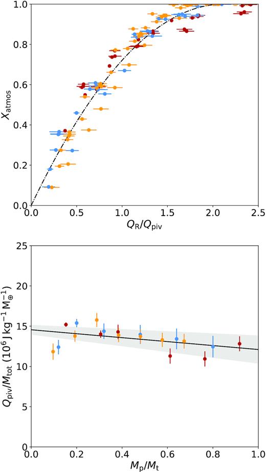
Top: Fractional atmosphere loss compared to specific impact energy scaled with respect to the pivot energy for each target mass. The amount of energy required to remove more atmosphere increases as the amount of atmosphere removed increases. Fitted to the data is a simple quadratic that has been fixed to cross the origin and have a peak at total atmosphere loss (equation 13). Bottom: Specific energy of the pivot normalized by the total mass of the system compared with projectile-target mass ratio. Mass normalized pivot energy appears to be approximately constant, decreasing slightly as projectile masses increase. The fit is given by equation (14).
Equation (14) has quite a shallow gradient, meaning that the energy of the pivot is strongly dependent on the the total mass, i.e. the impact energy is strongly dependent on the square of the total mass, implying it is related to the total g⊕tational binding energy of the system. The error envelope in Fig. 5 is generated from the variance of the fit parameters. Together equations (13) and (14) can be used to predict the mass fraction of atmosphere lost from the target for any head-on giant impact in the regime tested.
4 DISCUSSION
4.1 Caveats
4.1.1 Atmosphere fraction effects
We chose the initial atmosphere fraction for each target planet based on the most likely atmosphere fractions from the Bern global planet formation model (equation 1). One issue with this method is that it makes distinguishing between the effects of target mass and atmosphere fraction somewhat difficult, as both are directly related. An important result that requires further investigation is the relation between atmosphere fraction and pivot energy. One might expect that less massive atmospheres would require less energy to remove and thus core and mantle material would begin to be removed earlier, decreasing the pivot energy. We observe a decrease in pivot energy but we cannot distinguish whether this is due to a smaller atmosphere fraction or a shallower g⊕tational potential well from a less massive target. In future, we could test the cause of the decrease in pivot energy by simulating collisions involving targets of the same masses with different atmosphere fractions.
4.1.2 Equation of state effects
One simplification we have made in this work is to use ideal gas atmospheres as opposed to a more realistic EOS. For Earth atmospheric pressures this would have a negligible effect, but we are dealing with significantly more massive atmospheres (roughly 7 orders of magnitude). For such massive atmospheres, the pressures and densities at the base of the atmosphere are such that the assumption that molecules do not interact (inherent in using an ideal gas) may not be realistic. The lack of interparticle interactions means that we have unrealistically high densities at high pressures, (the base of our atmospheres post equilibration being 1.2–19.2 × 10⁵ atm or 1.2–19.2 × 10⁹ GPa). One effect of this is a significant compression of the atmosphere when equilibrating a gadget-2 planet. During the equilibration, the radii of atmospheres shrank on average by a factor of 2. Despite these issues, we have used an ideal gas as a starting point, more realistic EOS should be the subject of a future study.
4.1.3 Impact angle effects
For impact angle we have also elected to investigate the simplest case – head-on collisions. In general, we would expect an average collision angle of 45° (Shoemaker & Hackman 1962). Leinhardt & Stewart (2012) present in their prescription a method to relate the mass-loss of an off angle collision with a head-on one, which uses an interacting mass. In the impact scenarios considered in this work, we would expect the impact angle correction to become more complicated due to the density contrast between atmosphere and mantle. Hwang et al. (2017a,b) have previously done work on grazing collisions where the cores and mantles did not touch. Their results show that mass-loss follows a power-law dependence on impact parameter. We plan to investigate this further in future work.
4.2 Catastrophic disruption threshold scaling
Fig. 6 details how our results compare to Leinhardt & Stewart’s predictions. Our results run parallel to the prediction of equation (15) indicating a larger c* value of 2.52 (compared to the value given in Leinhardt & Stewart 2012). The larger c* means that a greater excess over the binding energy is required to remove material from planets with atmospheres than those without. This is presumably due to the increased compressibility and decreased viscosity of atmosphere compared to mantle and core material.
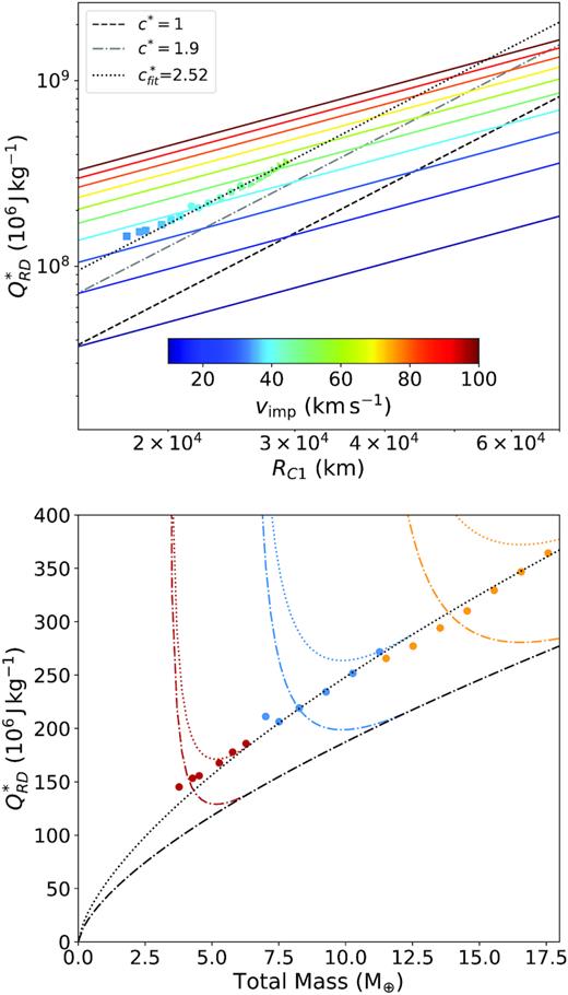
Top: Catastrophic disruption threshold |$Q_{\mathrm{RD}}^{*}$| compared with RC1 the radius a spherical body would have if it had the total system mass and a density of 1000 |$\mathrm{kg\, m^{-3}}$|, with the black and grey lines showing their predicted relationship for different values of the strength parameter c* following equation (15). We observe a value of c* = 2.52, which is a |$32{{\ \rm per\ cent}}$| increase compared to Leinhardt & Stewart (2012)’s value of 1.9 for solely rocky bodies. Coloured lines show the predicted catastrophic disruption threshold for equal mass collisions for particular velocities. The colour of each data point indicates the relative velocity the pair of planets would have for each collision if they were equal mass. Bottom: Comparison between the catastrophic disruption threshold, and the total mass of each set of collisions. The black lines detail predictions of the catastrophic disruption threshold for each total mass for pure energy scaling for different values of c*, the dotted is our measured value of 2.52, the dot–dashed is Leinhardt & Stewart (2012)’s value of 1.9, coloured lines show predictions for pure momentum scaling. Our results (the dots with colours representing target mass as per Fig. 4) appear to follow the prediction for pure energy scaling.
It should be noted that we appear to be observing pure energy scaling for these collisions as no mass ratio correction is required, this is illustrated best in the bottom part of Fig. 6. Here, the black lines represent the predicted catastrophic disruption threshold using energy scaling, whilst coloured lines represent the momentum scaling that Leinhardt & Stewart (2012) predict we should be close to. As can be observed, our results follow the energy scaled prediction closely. This runs contrary to the results in Leinhardt & Stewart (2012) that predict near-perfect momentum scaling. Presumably, this difference is due to the presence of the atmosphere, as the Leinhardt & Stewart (2012) method is based on Holsapple & Schmidt (1987)’s crater scaling, where they show that porous materials tend to follow momentum scaling, while perfect gases tend to follow energy scaling.
4.3 Mass-loss efficiency comparisons
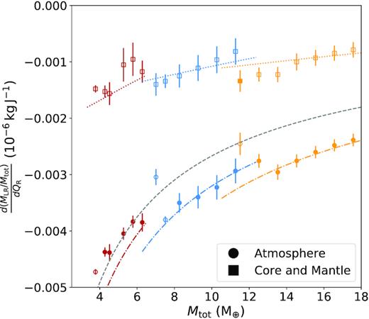
Comparisons between the mass-loss efficiency for core and mantle, and for atmosphere to the total mass of the system. Atmosphere loss shows a decreased efficiency in comparison to core and mantle loss, as might be expected considering the increased compressibilty of atmosphere material. The filled shapes are gradients where we obtained four or greater data points for that line, open are where we have three or fewer. The grey line shows the loss efficiency predicted by Leinhardt & Stewart (2012) for rocky material, the coloured line beneath them is this value multiplied by 1 plus the atmosphere fraction for that particular target as per equation (18). This appears to show reasonable correlation with our results especially for higher mass targets. The coloured dotted line above this shows a prediction of what the atmosphere gradient must be that uses all previously derived scaling laws, is linear and passes through zero mass-loss for zero input energy (equation 19). Our results show some degree of correlation with this value, but we do not have a high enough density of data in this region to effectively probe the accuracy of this prediction.
We can consider these gradients as a measurements of the efficiency of mass-loss in each regime. The efficiency of mass-loss for the core and mantle loss region is typically at least double that for the atmosphere-dominated loss regime, this is presumably due to the increased compressibility of the atmosphere.
As can be observed, the Leinhardt & Stewart (2012) model (equation 17 above) appears to underpredict the efficiency of mantle and core material loss for planets with substantial envelopes. This is likely due to the pressure of the atmosphere above providing a resisting force to reduce mantle loss. Once the atmosphere is removed, the specific energy of the impact is higher than would have been necessary to remove significant mantle if no atmosphere was present, so more material is being removed per unit of specific energy.
4.4 Implications
This study was motivated by the density disparity observed in exoplanet systems. The post-impact bodies in our simulations are hot and inflated, often with a large mass of vaporised silicate, and thus do not represent the structure of planets millions of years after their final giant impacts (Lock & Stewart 2017; Carter, Lock & Stewart 2020; Lock, Stewart & Ćuk 2020). To determine the bulk density of the remnants from their post-collision material composition, we use the approximation suggested in Lopez & Fortney (2014). In their model the total radius of a planet, Rplanet, from which we determine the density, can be calculated from summing the radial contributions of the following three components: the core and mantle, which has a power-law relation to mass; the convective envelope, which is dependent on the temperature of the atmosphere, which itself is a function of stellar flux and planet age; and the radiative atmosphere (also dependent on temperature). Here, we ignore the contribution of the radiative atmosphere due to its small effect (∼0.1R⊕). We used an age of |$5\, \mathrm{Gyr}$| for our comparison planets (see Fig. 8) as this is the most common age for stars in the local Galactic neighbourhood. We used a flux, Fplanet, of |$100\, \mathrm{F_{\oplus }}$| as the type of planets we simulated are most commonly observed at ∼0.1 au around the Sun-like stars. Fig. 8 shows contour plots of the radius (top) and density (bottom) as a function of mass and atmosphere fraction according to the Lopez & Fortney (2014) approximation described above.
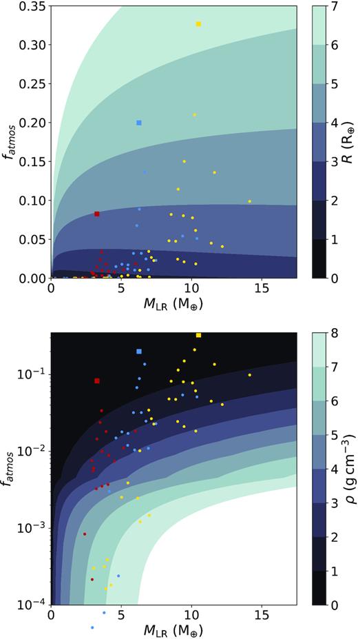
Top: Radius as a function of mass following the prescription of Lopez & Fortney (2014), compared against our initial targets (the squares) and also our post-collision largest remnants (the circles), the same colour scheme for target masses is used as for the rest of the paper. Bottom: Density as a function of mass calculated using the radius above, this is similarly compared against our initial targets (the squares) and also our post-collision largest remnants (the circles), collisions with full atmosphere removal have been removed so atmosphere fraction could be plotted logarithmically.
The prediction we obtained for the envelope radius of our initial targets using the Lopez & Fortney (2014) model was within 10 per cent of the radius of our initial thermodynamic profiles. This radius was, however, significantly larger than our gadget-2 targets due to the compression caused using an ideal gas. We also note that we could not reach the 20 mBar pressures which Lopez & Fortney (2014) consider to be the edge of the atmosphere with computationally practical resolutions.
For our collisions, we always observe a decrease in atmosphere fraction. This decrease in atmosphere fraction means that for all the collisions we simulate, except for those resulting in largest remnants below the resolution limit, we observe an increase in density as shown in the bottom panel of Fig. 8.
4.5 New prescriptions for atmosphere loss and largest remnant mass
Here, we summarize the process one would need to use to predict the atmosphere loss from any giant impact in the regime probed by this paper, as well as the modifications to the Leinhardt & Stewart (2012) prescription for largest post-collision remnant mass for an arbitrary head on collision between a mini-Neptune with a significant gaseous envelope and a lower mass super-Earth without an atmosphere. This algorithm can be incorporated into N-body codes and population synthesis models.
- For a given collision scenario (Mp, Mt, and Vimp), calculate the specific relative kinetic energy of the impact,where Mtot = Mt + Mp, and μ = MtMp/(Mt + Mp) is the reduced mass, Mt is the target mass, Mp the projectile mass, and Vimp is the impact velocity.(20)$$\begin{eqnarray*} Q_\mathrm{R}=\frac{1}{2}\mu \frac{V_\mathrm{imp}^2}{M_{\mathrm{tot}}}, \end{eqnarray*}$$
- Then, calculate the specific kinetic energy of the transition between the atmosphere loss and core and mantle loss regimes:(21)$$\begin{eqnarray*} Q_{\mathrm{piv}}=\left(\frac{M_{\mathrm{tot}}}{M_\oplus }\right)\left(-2.45\frac{M_\mathrm{p}}{M_\mathrm{t}}+14.56\right) \,\,\,\, [10^6\, \mathrm{J\, kg^{-1}}]. \end{eqnarray*}$$
- Calculate the catastrophic disruption threshold,using a value of c* = 2.52 for collisions involving planets with atmospheres (|$Q_{\mathrm{RD}}^{*(\mathrm{New})}$|) and c* = 1.9 (|$Q_{\mathrm{RD}}^{*(\mathrm{LS12})}$|, as in Leinhardt & Stewart 2012) for targets with no atmosphere. |$\rho _{\mathrm{1}}=1000\, \mathrm{kg\, m^{-3}}$|, and |$R_{\mathrm{C1}} = \left(\frac{3M_{\mathrm{tot}}}{4\pi \rho _{\mathrm{1}}}\right)^{\frac{1}{3}}$| is the radius a spherical body would have if it had the total system mass and a density of ρ1.(22)$$\begin{eqnarray*} Q_{\mathrm{RD}}^{*}=c^*\frac{4}{5}\pi \rho _{\mathrm{1}}GR_{\mathrm{C1}}^2, \end{eqnarray*}$$
- Calculate the gradients of each of the linear sections of the largest remnant mass fraction relation. For the core and mantle loss regime this iswhere fatmos is the mass fraction of the target which is atmosphere.(23)$$\begin{eqnarray*} m_{\mathrm{c\&m}}=\frac{-0.5(1+f_{\mathrm{atmos}})}{Q_{\mathrm{RD}}^{*(\mathrm{LS12})}} , \end{eqnarray*}$$
- Zero impact energy means zero mass-loss therefore the gradient for the atmosphere loss dominated part of the relation is, from equation (9),(24)$$\begin{eqnarray*} m_{\mathrm{atmos}}=\frac{m_{\mathrm{c\&m}}\left(Q_{\mathrm{piv}}-Q_{\mathrm{RD}}^{*(\mathrm{New})}\right)-0.5}{Q_{\mathrm{piv}}}. \end{eqnarray*}$$
- Next, calculate the supercatastrophic disruption threshold, taking this to be where <10 per cent of the initial mass ends up in the largest remnant (following Leinhardt & Stewart 2012) we obtain(25)$$\begin{eqnarray*} Q_{\mathrm{supercat}}=Q_{\mathrm{RD}}^{*(\mathrm{New})}-\frac{0.4}{m_{\mathrm{c\&m}}}. \end{eqnarray*}$$
- Then, the total mass in the largest remnant isWe did not probe the supercatastrophic disruption regime in this study due as this would require much higher resolution; for collisions in this energy regime we recommend using the prescription of Leinhardt & Stewart (2012).(26)$$\begin{eqnarray*} \frac{M_{\mathrm{LR}}}{M_{\mathrm{tot}}}= \left\lbrace \begin{array}{@{}l@{\quad }l@{}}m_{\mathrm{atmos}}Q_{\mathrm{R}}+1 & 0\lt Q_{\mathrm{R}}\lt Q_{\mathrm{piv}} \\ \\ m_{\mathrm{c\&m}}\left(Q_{\mathrm{R}}-Q_{\mathrm{RD}}^{*(\mathrm{New})}\right)+0.5 & Q_{\mathrm{piv}}\lt Q_{\mathrm{R}}\lt Q_{\mathrm{supercat}}.\\ \end{array}\right. \nonumber\\ \end{eqnarray*}$$
- Finally, the atmosphere fraction lost is(27)$$\begin{eqnarray*} \chi _{\mathrm{loss}}^{\mathrm{atmos}} = \left\lbrace \begin{array}{@{}l@{\quad }l@{}}\frac{-0.94^2}{4}\left(\frac{Q_{\mathrm{R}}}{Q_{\mathrm{piv}}}\right)^{2}+0.94\frac{Q_{\mathrm{R}}}{Q_{\mathrm{piv}}} & \frac{Q_{\mathrm{R}}}{Q_{\mathrm{piv}}}\lt 2.12 \\ 1 & \frac{Q_{\mathrm{R}}}{Q_{\mathrm{piv}}}\gt 2.12. \end{array}\right. \end{eqnarray*}$$
5 SUMMARY
In this paper, we present the results from a series of sph simulations of head-on collisions of planets in which the target has a significant atmosphere. Our findings are summarized next:
Giant impacts can have sufficient energy to remove large fractions of mass from the target planet; the mass lost is dependent upon the specific kinetic energy of the impact.
Giant impacts can result in substantial increases in the densities of mini-Neptune planets by ejecting a fraction of their atmospheres.
The fraction of mass lost splits into two regimes – at low specific impact energies only the outer layers are ejected corresponding to atmosphere dominated loss, at higher energies material deeper in the potential is excavated resulting in significant core and mantle loss.
Approximately 20 per cent of the initial atmosphere remains at the transition between the two regimes.
A single collision cannot remove all the atmosphere without also removing a significant percentage of mantle material.
Mass removal is less efficient in the atmosphere loss dominated regime compared to the core and mantle loss regime.
The specific energy of this transition (pivot energy, Qpiv) scales linearly with the ratio of projectile to target mass for all projectile-target mass ratios measured:
|$Q_{\mathrm{piv}}=M_{\mathrm{tot}}\left(-2.45\frac{M_\mathrm{p}}{M_\mathrm{t}}+14.56\right) \,\,\,\,\big[10^6\, \mathrm{J\, kg^{-1}\, M_\oplus ^{-1}}\big]$|.
The fraction of atmosphere lost is well approximated by a quadratic in terms of the ratio of specific energy to transition energy: |$X_{\mathrm{loss}}^{\mathrm{atmos}} = \frac{-0.94^2}{4}\left(\frac{Q_{\mathrm{R}}}{Q_{\mathrm{piv}}}\right)^{2}+0.94\frac{Q_{\mathrm{R}}}{Q_{\mathrm{piv}}}$|, for |$Q_{\mathrm{R}}\lt 2.12\, Q_{\mathrm{piv}}$|, and total atmosphere loss for energies greater than this.
SUPPORTING INFORMATION
http://www.star.bris.ac.uk/TDenman/Paper1_Videos/
Please note: Oxford University Press is not responsible for the content or functionality of any supporting materials supplied by the authors. Any queries (other than missing material) should be directed to the corresponding author for the article.
ACKNOWLEDGEMENTS
This work was carried out using the computational facilities of the Advanced Computing Research Centre, University of Bristol – http://www.bristol.ac.uk/acrc/. Thomas R. Denman acknowledges support from an STFC (Science and Technologies Facilities Council) studentship. Phil J. Carter acknowledges support from University of California Office of the President grant LFR-17-449059. Christoph Mordasini acknowledges support from the Swiss National Science Foundation under grant BSSGI0_155816 ‘PlanetsInTime’. Parts of this work have been carried out within the framework of the NCCR PlanetS (National Centre of Competence in Research PlanetS) supported by the Swiss National Science Foundation. This research has used the NASA Exoplanet Archive, which is operated by the California Institute of Technology, under contract with the National Aeronautics and Space Administration under the Exoplanet Exploration Program.
REFERENCES
APPENDIX:
FURTHER IMPACTS
We present results in this paper for collisions against three separate simulated super-Earth targets, a |$3.27\, \mathrm{M}_{\oplus }$| target with a |$0.27\, \mathrm{M_{\oplus }}$| atmosphere, |$1\, \mathrm{M_{\oplus }}$| core, and |$2\, \mathrm{M_{\oplus }}$| mantle (initial conditions and results given in Table A1); a |$6.26\, \mathrm{M}_{\oplus }$| one with a |$1.25\, \mathrm{M_{\oplus }}$| atmosphere, |$1.67\, \mathrm{M_{\oplus }}$| core, and |$3.34\, \mathrm{M_{\oplus }}$| mantle (Table 1); and a |$10.5\, \mathrm{M}_{\oplus }$| one with a |$3.43\, \mathrm{M_{\oplus }}$| atmosphere, |$2.36\, \mathrm{M_{\oplus }}$| core, and |$4.71\, \mathrm{M_{\oplus }}$| mantle (Table A2).
Parameters for head-on collisions between a |$3.27\, \mathrm{M}_{\oplus }$| target (|$M_\mathrm{t}^{\mathrm{core}} = 3.0 \, \mathrm{M}_{\oplus }$|, |$M_\mathrm{t}^{\mathrm{atmos}} = 0.27 \, \mathrm{M}_{\oplus }$|) with a mantle surface radius of |$1.31\, \mathrm{R}_{\oplus }$|, and an atmosphere scale height of |$0.52\, \mathrm{R}_{\oplus }$|, and projectiles of mass Mp. Similar to Tables 1 and A2.
| ID | Mp | Rp | |$v_{\mathrm{imp}}^{\mathrm{pred}}$| | |$\frac{v_{\mathrm{imp}}^{\mathrm{pred}}}{v_{\mathrm{esc}}}$| | |$v_{\mathrm{imp}}^{\mathrm{meas}}$| | |$\frac{v_{\mathrm{imp}}^{\mathrm{meas}}}{v_{\mathrm{esc}}}$| | vinit | |$\frac{v_{\mathrm{init}}}{v_{\mathrm{esc}}}$| | S | MLR | |$M_{\mathrm{LR}}^{\mathrm{atmos}}$| | |$M_{\mathrm{LR}}^{\mathrm{core}}$| | |$\frac{M_{\mathrm{LR}}}{M_{\mathrm{tot}}}$| | |$X_{\mathrm{loss}}^{\mathrm{atmos}}$| | |$X_{\mathrm{loss}}^{\mathrm{c\&m}}$| | Category |
|---|---|---|---|---|---|---|---|---|---|---|---|---|---|---|---|---|
| (M⊕) | (R⊕) | (|$\mathrm{km}\, \mathrm{s}^{-1}$|) | (|$\mathrm{km}\, \mathrm{s}^{-1}$|) | (|$\mathrm{km}\, \mathrm{s}^{-1}$|) | (R⊕) | (M⊕) | (M⊕) | (M⊕) | ||||||||
| 3–0 | 0.50 | 0.78 | 20.00 | 1.46 | 19.28 | 1.41 | 14.98 | 1.10 | 9.59 | 3.66 | 0.17 | 3.49 | 0.97 | 0.37 | 0.0 | AL-CM |
| 3–1 | 0.50 | 0.78 | 25.00 | 1.83 | 24.32 | 1.78 | 21.20 | 1.55 | 9.59 | 3.59 | 0.12 | 3.47 | 0.95 | 0.56 | 0.01 | AL-CM |
| 3–2 | 0.50 | 0.78 | 30.00 | 2.19 | 29.31 | 2.14 | 26.92 | 1.97 | 9.59 | 3.49 | 0.08 | 3.41 | 0.92 | 0.7 | 0.03 | AL-CM |
| 3–3 | 0.50 | 0.78 | 35.00 | 2.56 | 34.29 | 2.51 | 32.39 | 2.37 | 9.60 | 3.27 | 0.05 | 3.22 | 0.87 | 0.81 | 0.08 | AL-CA |
| 3–4 | 0.50 | 0.78 | 40.00 | 2.92 | 39.25 | 2.87 | 37.74 | 2.76 | 9.59 | 2.90 | 0.02 | 2.88 | 0.77 | 0.93 | 0.18 | AL-CE |
| 3–5 | 0.50 | 0.78 | 50.00 | 3.66 | 49.14 | 3.59 | 48.21 | 3.53 | 9.59 | 2.00 | 0.00 | 2.00 | 0.53 | 1.0 | 0.43 | TAL-CE |
| 3–6 | 1.00 | 0.97 | 20.00 | 1.40 | 19.30 | 1.35 | 14.77 | 1.04 | 10.13 | 4.07 | 0.11 | 3.96 | 0.95 | 0.59 | 0.01 | AL-CM |
| 3–7 | 1.00 | 0.97 | 25.00 | 1.75 | 24.37 | 1.71 | 21.05 | 1.48 | 10.12 | 3.92 | 0.07 | 3.85 | 0.92 | 0.74 | 0.04 | AL-CM |
| 3–8 | 1.00 | 0.97 | 30.00 | 2.10 | 29.40 | 2.06 | 26.80 | 1.88 | 10.14 | 3.55 | 0.04 | 3.51 | 0.83 | 0.85 | 0.12 | AL-CA |
| 3–9 | 1.00 | 0.97 | 35.00 | 2.46 | 34.41 | 2.41 | 32.30 | 2.27 | 10.13 | 3.03 | 0.02 | 3.01 | 0.71 | 0.93 | 0.25 | AL-CA |
| 3–10 | 1.00 | 0.97 | 40.00 | 2.81 | 39.39 | 2.76 | 37.66 | 2.64 | 10.12 | 2.40 | 0.00 | 2.40 | 0.56 | 1.0 | 0.4 | TAL-CE |
| 3–11 | 1.00 | 0.97 | 50.00 | 3.51 | 49.31 | 3.46 | 48.15 | 3.38 | 10.14 | 0.32 | 0.00 | 0.32 | 0.07 | 1.0 | 0.92 | SCD |
| 3–12 | 1.25 | 1.03 | 20.00 | 1.38 | 19.29 | 1.33 | 14.60 | 1.00 | 10.31 | 4.30 | 0.11 | 4.19 | 0.95 | 0.59 | 0.02 | AL-CM |
| 3–13 | 1.25 | 1.03 | 25.00 | 1.72 | 24.39 | 1.68 | 20.93 | 1.44 | 10.31 | 4.08 | 0.06 | 4.02 | 0.9 | 0.78 | 0.06 | AL-CA |
| 3–14 | 1.25 | 1.03 | 30.00 | 2.06 | 29.43 | 2.03 | 26.70 | 1.84 | 10.31 | 3.64 | 0.04 | 3.60 | 0.8 | 0.85 | 0.15 | AL-CA |
| 3–15 | 1.25 | 1.03 | 35.00 | 2.41 | 34.43 | 2.37 | 32.22 | 2.22 | 10.31 | 2.98 | 0.02 | 2.97 | 0.66 | 0.93 | 0.3 | AL-CE |
| 3–16 | 1.25 | 1.03 | 40.00 | 2.75 | 39.42 | 2.71 | 37.59 | 2.59 | 10.32 | 2.27 | 0.00 | 2.27 | 0.5 | 1.0 | 0.47 | TAL-CE |
| 3–17 | 1.25 | 1.03 | 50.00 | 3.44 | 49.35 | 3.40 | 48.09 | 3.31 | 10.31 | – | – | – | – | 1.0 | – | SCD |
| 3–18 | 2.00 | 1.18 | 20.00 | 1.31 | 19.32 | 1.26 | 14.03 | 0.92 | 10.77 | 5.03 | 0.11 | 4.92 | 0.95 | 0.59 | 0.02 | AL-CM |
| 3–19 | 2.00 | 1.18 | 25.00 | 1.63 | 24.38 | 1.59 | 20.54 | 1.34 | 10.78 | 4.69 | 0.06 | 4.63 | 0.89 | 0.78 | 0.07 | AL-CA |
| 3–20 | 2.00 | 1.18 | 30.00 | 1.96 | 29.42 | 1.92 | 26.39 | 1.73 | 10.79 | 4.10 | 0.04 | 4.06 | 0.78 | 0.85 | 0.19 | AL-CA |
| 3–21 | 2.00 | 1.18 | 35.00 | 2.29 | 34.46 | 2.25 | 31.96 | 2.09 | 10.78 | 3.23 | 0.01 | 3.21 | 0.61 | 0.96 | 0.36 | TAL-CA |
| 3–22 | 2.00 | 1.18 | 40.00 | 2.62 | 39.46 | 2.58 | 37.37 | 2.44 | 10.78 | 2.29 | 0.00 | 2.29 | 0.43 | 1.0 | 0.54 | TAL-CE |
| 3–23 | 2.00 | 1.18 | 50.00 | 3.27 | 49.42 | 3.23 | 47.92 | 3.13 | 10.79 | – | – | – | – | 1.0 | – | SCD |
| 3–24 | 2.50 | 1.26 | 20.00 | 1.27 | 19.27 | 1.22 | 13.59 | 0.86 | 11.01 | 5.52 | 0.11 | 5.41 | 0.96 | 0.59 | 0.02 | AL-CM |
| 3–25 | 2.50 | 1.26 | 25.00 | 1.59 | 24.42 | 1.55 | 20.24 | 1.28 | 11.01 | 5.16 | 0.06 | 5.10 | 0.89 | 0.78 | 0.07 | AL-CA |
| 3–26 | 2.50 | 1.26 | 30.00 | 1.90 | 29.46 | 1.87 | 26.17 | 1.66 | 11.01 | 4.52 | 0.03 | 4.48 | 0.78 | 0.89 | 0.19 | AL-CA |
| 3–27 | 2.50 | 1.26 | 35.00 | 2.22 | 34.47 | 2.19 | 31.78 | 2.02 | 11.00 | 3.62 | 0.01 | 3.61 | 0.63 | 0.96 | 0.34 | TAL-CA |
| 3–28 | 2.50 | 1.26 | 40.00 | 2.54 | 39.47 | 2.50 | 37.21 | 2.36 | 11.01 | 2.56 | 0.00 | 2.56 | 0.44 | 1.0 | 0.53 | TAL-CE |
| 3–29 | 3.00 | 1.33 | 20.00 | 1.23 | 19.20 | 1.19 | 13.14 | 0.81 | 11.20 | 6.01 | 0.11 | 5.90 | 0.96 | 0.59 | 0.02 | AL-CM |
| 3–30 | 3.00 | 1.33 | 25.00 | 1.54 | 24.38 | 1.50 | 19.94 | 1.23 | 11.21 | 5.68 | 0.07 | 5.61 | 0.91 | 0.74 | 0.07 | AL-CA |
| 3–31 | 3.00 | 1.33 | 30.00 | 1.85 | 29.43 | 1.82 | 25.93 | 1.60 | 11.22 | 5.01 | 0.04 | 4.97 | 0.8 | 0.85 | 0.17 | AL-CA |
| 3–32 | 3.00 | 1.33 | 35.00 | 2.16 | 34.46 | 2.13 | 31.58 | 1.95 | 11.21 | 4.06 | 0.02 | 4.04 | 0.65 | 0.93 | 0.33 | AL-CA |
| 3–33 | 3.00 | 1.33 | 40.00 | 2.47 | 39.47 | 2.44 | 37.05 | 2.29 | 11.22 | 2.93 | 0.00 | 2.93 | 0.47 | 1.0 | 0.51 | TAL-CE |
| 3–34 | 3.00 | 1.33 | 50.00 | 3.09 | 49.45 | 3.05 | 47.67 | 2.94 | 11.21 | – | – | – | – | 1.0 | – | SCD |
A summary of collision parameters and results for head-on collisions between a |$10.50\, \mathrm{M}_{\oplus }$| target (|$M_\mathrm{t}^{\mathrm{core}} = 7.07 \, \mathrm{M}_{\oplus }$|, |$M_\mathrm{t}^{\mathrm{atmos}} = 3.43 \, \mathrm{M}_{\oplus }$|) with a mantle surface radius of |$1.60\, \mathrm{R}_{\oplus }$|, and an atmosphere scale height of |$0.70\, \mathrm{R}_{\oplus }$|, and projectiles of mass Mp. Similar to Tables 1 and A1.
| ID | Mp | Rp | |$v_{\mathrm{imp}}^{\mathrm{pred}}$| | |$\frac{v_{\mathrm{imp}}^{\mathrm{pred}}}{v_{\mathrm{esc}}}$| | |$v_{\mathrm{imp}}^{\mathrm{meas}}$| | |$\frac{v_{\mathrm{imp}}^{\mathrm{meas}}}{v_{\mathrm{esc}}}$| | vinit | |$\frac{v_{\mathrm{init}}}{v_{\mathrm{esc}}}$| | S | MLR | |$M_{\mathrm{LR}}^{\mathrm{atmos}}$| | |$M_{\mathrm{LR}}^{\mathrm{core}}$| | |$\frac{M_{\mathrm{LR}}}{M_{\mathrm{tot}}}$| | |$X_{\mathrm{loss}}^{\mathrm{atmos}}$| | |$X_{\mathrm{loss}}^{\mathrm{c\&m}}$| | Category |
|---|---|---|---|---|---|---|---|---|---|---|---|---|---|---|---|---|
| (M⊕) | (R⊕) | (|$\mathrm{km}\, \mathrm{s}^{-1}$|) | (|$\mathrm{km}\, \mathrm{s}^{-1}$|) | (|$\mathrm{km}\, \mathrm{s}^{-1}$|) | (R⊕) | (M⊕) | (M⊕) | (M⊕) | ||||||||
| 7–0 | 1.01 | 0.95 | 30.00 | 1.51 | 27.76 | 1.39 | 21.07 | 1.06 | 13.54 | 11.20 | 3.12 | 8.08 | 0.97 | 0.09 | 0.0 | AL-CM |
| 7–1 | 1.01 | 0.95 | 40.00 | 2.01 | 37.18 | 1.87 | 33.82 | 1.70 | 13.54 | 10.81 | 2.73 | 8.08 | 0.94 | 0.2 | 0.0 | AL-CM |
| 7–2 | 1.01 | 0.95 | 50.00 | 2.51 | 46.47 | 2.33 | 45.21 | 2.27 | 13.55 | 10.22 | 2.15 | 8.07 | 0.89 | 0.37 | 0.0 | AL-CM |
| 7–3 | 1.01 | 0.95 | 55.00 | 2.76 | 51.12 | 2.57 | 50.68 | 2.54 | 13.57 | 9.85 | 1.79 | 8.07 | 0.86 | 0.48 | 0.0 | AL-CM |
| 7–4 | 1.01 | 0.95 | 60.00 | 3.01 | 55.99 | 2.81 | 56.07 | 2.81 | 13.57 | 9.48 | 1.42 | 8.06 | 0.82 | 0.59 | 0.0 | AL-CM |
| 7–5 | 1.01 | 0.95 | 65.00 | 3.26 | 60.57 | 3.04 | 61.39 | 3.08 | 13.56 | 9.05 | 1.03 | 8.01 | 0.79 | 0.7 | 0.01 | AL-CM |
| 7–6 | 1.01 | 0.95 | 70.00 | 3.51 | 65.18 | 3.27 | 66.66 | 3.35 | 13.58 | 8.55 | 0.70 | 7.85 | 0.74 | 0.8 | 0.03 | AL-CM |
| 7–7 | 1.01 | 0.95 | 80.00 | 4.01 | 74.50 | 3.74 | 77.10 | 3.87 | 13.55 | 6.96 | 0.24 | 6.72 | 0.6 | 0.93 | 0.17 | AL-CE |
| 7–8 | 2.02 | 1.17 | 30.00 | 1.46 | 28.16 | 1.37 | 21.11 | 1.03 | 14.17 | 11.85 | 2.76 | 9.09 | 0.95 | 0.2 | 0.0 | AL-CM |
| 7–9 | 2.02 | 1.17 | 40.00 | 1.95 | 37.80 | 1.84 | 33.85 | 1.65 | 14.19 | 11.03 | 1.96 | 9.08 | 0.88 | 0.43 | 0.0 | AL-CM |
| 7–10 | 2.02 | 1.17 | 50.00 | 2.44 | 47.32 | 2.31 | 45.23 | 2.21 | 14.18 | 10.15 | 1.16 | 8.98 | 0.81 | 0.66 | 0.01 | AL-CM |
| 7–11 | 2.02 | 1.17 | 55.00 | 2.68 | 52.02 | 2.54 | 50.70 | 2.47 | 14.19 | 9.42 | 0.76 | 8.66 | 0.75 | 0.78 | 0.05 | AL-CM |
| 7–12 | 2.02 | 1.17 | 60.00 | 2.93 | 56.64 | 2.76 | 56.09 | 2.74 | 14.19 | 8.40 | 0.40 | 7.99 | 0.67 | 0.88 | 0.12 | AL-CA |
| 7–13 | 2.02 | 1.17 | 65.00 | 3.17 | 61.47 | 3.00 | 61.41 | 3.00 | 14.16 | 7.14 | 0.19 | 6.95 | 0.57 | 0.94 | 0.24 | AL-CE |
| 7–14 | 2.02 | 1.17 | 70.00 | 3.42 | 66.26 | 3.23 | 66.67 | 3.25 | 14.21 | 5.47 | 0.02 | 5.45 | 0.44 | 0.99 | 0.4 | TAL-CE |
| 7–15 | 2.02 | 1.17 | 80.00 | 3.90 | 75.81 | 3.70 | 77.11 | 3.76 | 14.19 | 1.65 | 0.00 | 1.65 | 0.13 | 1.0 | 0.82 | TAL-CE |
| 7–16 | 3.03 | 1.32 | 30.00 | 1.43 | 28.33 | 1.35 | 20.89 | 0.99 | 14.62 | 12.58 | 2.49 | 10.09 | 0.93 | 0.27 | 0.0 | AL-CM |
| 7–17 | 3.03 | 1.32 | 40.00 | 1.90 | 38.07 | 1.81 | 33.71 | 1.60 | 14.61 | 11.63 | 1.58 | 10.05 | 0.86 | 0.54 | 0.01 | AL-CM |
| 7–18 | 3.03 | 1.32 | 50.00 | 2.38 | 47.68 | 2.27 | 45.13 | 2.15 | 14.64 | 10.07 | 0.78 | 9.28 | 0.74 | 0.77 | 0.08 | AL-CA |
| 7–19 | 3.03 | 1.32 | 55.00 | 2.62 | 52.50 | 2.50 | 50.61 | 2.41 | 14.65 | 8.87 | 0.42 | 8.45 | 0.66 | 0.88 | 0.16 | AL-CA |
| 7–20 | 3.03 | 1.32 | 60.00 | 2.85 | 57.25 | 2.72 | 56.00 | 2.66 | 14.64 | 7.31 | 0.17 | 7.15 | 0.54 | 0.95 | 0.29 | TAL-CA |
| 7–21 | 3.03 | 1.32 | 65.00 | 3.09 | 62.05 | 2.95 | 61.33 | 2.92 | 14.65 | 5.02 | 0.01 | 5.01 | 0.37 | 1.0 | 0.5 | TAL-CE |
| 7–22 | 3.03 | 1.32 | 70.00 | 3.33 | 66.78 | 3.18 | 66.61 | 3.17 | 14.62 | 3.05 | 0.00 | 3.05 | 0.23 | 1.0 | 0.7 | TAL-CE |
| 7–23 | 3.03 | 1.32 | 80.00 | 3.80 | 76.41 | 3.63 | 77.05 | 3.66 | 14.64 | – | – | – | – | 1.0 | – | SCD |
| 7–24 | 4.04 | 1.43 | 30.00 | 1.39 | 28.37 | 1.32 | 20.53 | 0.95 | 14.94 | 13.41 | 2.31 | 11.10 | 0.92 | 0.33 | 0.0 | AL-CM |
| 7–25 | 4.04 | 1.43 | 40.00 | 1.86 | 38.19 | 1.77 | 33.49 | 1.55 | 14.95 | 12.39 | 1.43 | 10.96 | 0.85 | 0.58 | 0.01 | AL-CM |
| 7–26 | 4.04 | 1.43 | 50.00 | 2.32 | 47.91 | 2.22 | 44.96 | 2.09 | 14.97 | 10.29 | 0.63 | 9.66 | 0.71 | 0.82 | 0.13 | AL-CA |
| 7–27 | 4.04 | 1.43 | 55.00 | 2.55 | 52.72 | 2.45 | 50.46 | 2.34 | 14.94 | 8.81 | 0.30 | 8.51 | 0.61 | 0.91 | 0.23 | AL-CA |
| 7–28 | 4.04 | 1.43 | 60.00 | 2.79 | 57.57 | 2.67 | 55.87 | 2.59 | 14.96 | 6.32 | 0.06 | 6.25 | 0.43 | 0.98 | 0.44 | TAL-CE |
| 7–29 | 4.04 | 1.43 | 65.00 | 3.02 | 62.36 | 2.89 | 61.20 | 2.84 | 14.98 | 4.01 | 0.00 | 4.01 | 0.28 | 1.0 | 0.64 | TAL-CE |
| 7–30 | 4.04 | 1.43 | 70.00 | 3.25 | 67.15 | 3.12 | 66.49 | 3.09 | 14.98 | 1.75 | 0.00 | 1.75 | 0.12 | 1.0 | 0.84 | TAL-CE |
| 7–31 | 4.04 | 1.43 | 80.00 | 3.71 | 76.75 | 3.56 | 76.95 | 3.57 | 14.99 | – | – | – | – | 1.0 | – | SCD |
| 7–32 | 5.05 | 1.52 | 30.00 | 1.36 | 28.40 | 1.29 | 20.11 | 0.91 | 15.21 | 14.36 | 2.25 | 12.11 | 0.92 | 0.34 | 0.0 | AL-CM |
| 7–33 | 5.05 | 1.52 | 40.00 | 1.82 | 38.24 | 1.74 | 33.23 | 1.51 | 15.22 | 13.19 | 1.38 | 11.81 | 0.85 | 0.6 | 0.03 | AL-CM |
| 7–34 | 5.05 | 1.52 | 50.00 | 2.27 | 48.01 | 2.18 | 44.77 | 2.03 | 15.21 | 10.73 | 0.55 | 10.18 | 0.69 | 0.84 | 0.16 | AL-CA |
| 7–35 | 5.05 | 1.52 | 55.00 | 2.50 | 52.85 | 2.40 | 50.29 | 2.28 | 15.24 | 9.01 | 0.22 | 8.79 | 0.58 | 0.94 | 0.27 | AL-CA |
| 7–36 | 5.05 | 1.52 | 60.00 | 2.72 | 57.69 | 2.62 | 55.71 | 2.53 | 15.25 | 6.17 | 0.02 | 6.16 | 0.4 | 0.99 | 0.49 | TAL-CE |
| 7–37 | 5.05 | 1.52 | 65.00 | 2.95 | 62.53 | 2.84 | 61.07 | 2.77 | 15.25 | 3.78 | 0.00 | 3.77 | 0.24 | 1.0 | 0.69 | TAL-CE |
| 7–38 | 5.05 | 1.52 | 70.00 | 3.18 | 67.35 | 3.06 | 66.37 | 3.01 | 15.21 | 1.65 | 0.00 | 1.65 | 0.11 | 1.0 | 0.86 | TAL-CE |
| 7–39 | 5.05 | 1.52 | 80.00 | 3.63 | 77.01 | 3.50 | 76.84 | 3.49 | 15.25 | – | – | – | – | 1.0 | – | SCD |
| 7–40 | 6.06 | 1.60 | 30.00 | 1.33 | 28.39 | 1.26 | 19.67 | 0.87 | 15.46 | 15.33 | 2.22 | 13.11 | 0.93 | 0.35 | 0.0 | AL-CM |
| 7–41 | 6.06 | 1.60 | 40.00 | 1.78 | 38.27 | 1.70 | 32.97 | 1.47 | 15.46 | 14.14 | 1.40 | 12.74 | 0.85 | 0.59 | 0.03 | AL-CM |
| 7–42 | 6.06 | 1.60 | 50.00 | 2.22 | 48.04 | 2.14 | 44.57 | 1.98 | 15.47 | 11.40 | 0.51 | 10.89 | 0.69 | 0.85 | 0.17 | AL-CA |
| 7–43 | 6.06 | 1.60 | 55.00 | 2.44 | 52.96 | 2.35 | 50.12 | 2.23 | 15.46 | 9.47 | 0.20 | 9.27 | 0.57 | 0.94 | 0.29 | AL-CA |
| 7–44 | 6.06 | 1.60 | 60.00 | 2.67 | 57.82 | 2.57 | 55.56 | 2.47 | 15.48 | 6.35 | 0.01 | 6.34 | 0.38 | 1.0 | 0.52 | TAL-CE |
| 7–45 | 6.06 | 1.60 | 65.00 | 2.89 | 62.62 | 2.78 | 60.92 | 2.71 | 15.46 | 3.90 | 0.00 | 3.90 | 0.24 | 1.0 | 0.7 | TAL-CE |
| 7–46 | 6.06 | 1.60 | 70.00 | 3.11 | 67.50 | 3.00 | 66.23 | 2.94 | 15.49 | 1.78 | 0.00 | 1.78 | 0.11 | 1.0 | 0.86 | TAL-CE |
| 7–47 | 6.06 | 1.60 | 80.00 | 3.56 | 77.14 | 3.43 | 76.72 | 3.41 | 15.50 | – | – | – | – | 1.0 | – | SCD |
| 7–48 | 7.07 | 1.67 | 30.00 | 1.31 | 28.38 | 1.24 | 19.18 | 0.84 | 15.67 | 16.30 | 2.18 | 14.12 | 0.93 | 0.36 | 0.0 | AL-CM |
| 7–49 | 7.07 | 1.67 | 40.00 | 1.74 | 38.30 | 1.67 | 32.68 | 1.42 | 15.67 | 15.10 | 1.36 | 13.75 | 0.86 | 0.6 | 0.03 | AL-CM |
| 7–50 | 7.07 | 1.67 | 50.00 | 2.18 | 48.10 | 2.10 | 44.36 | 1.93 | 15.67 | 12.19 | 0.50 | 11.69 | 0.69 | 0.85 | 0.17 | AL-CA |
| 7–51 | 7.07 | 1.67 | 55.00 | 2.40 | 52.98 | 2.31 | 49.93 | 2.18 | 15.65 | 10.30 | 0.19 | 10.11 | 0.59 | 0.94 | 0.29 | AL-CA |
| 7–52 | 7.07 | 1.67 | 60.00 | 2.61 | 57.85 | 2.52 | 55.39 | 2.41 | 15.66 | 7.00 | 0.01 | 6.99 | 0.4 | 1.0 | 0.51 | TAL-CE |
| 7–53 | 7.07 | 1.67 | 65.00 | 2.83 | 62.66 | 2.73 | 60.77 | 2.65 | 15.70 | 4.27 | 0.00 | 4.26 | 0.24 | 1.0 | 0.7 | TAL-CE |
| 7–54 | 7.07 | 1.67 | 70.00 | 3.05 | 67.55 | 2.94 | 66.09 | 2.88 | 15.69 | 2.23 | 0.00 | 2.23 | 0.13 | 1.0 | 0.84 | TAL-CE |
| 7–55 | 7.07 | 1.67 | 80.00 | 3.49 | 77.25 | 3.37 | 76.60 | 3.34 | 15.67 | – | – | – | – | 1.0 | – | SCD |
