


ABSTRACT
Magnetic fields of strongly magnetized stars can trap conducting matter due to frozen-in condition. In the force-free regime, the motion of the matter along the field lines may be considered in the ‘bead on a wire’ approximation. Such a motion, if gravity and centrifugal forces are taken into account, has equilibrium points, some of which are stable. In most cases, stability is possible in about several per cent of the possible locations. Corresponding oscillation frequencies span the range from zero to |$\sqrt{3}$| of the spin frequency. We suggest that this variability mode may be excited in some X-ray pulsars during the outbursts and create the peaked broad-band noise component near the break frequency in the power density spectrum, as well as produce some of the quasi-periodic oscillation features in this frequency range. Existence of this variability does not require any changes in mass accretion rate and involves only a small amount of matter infiltrating from the disc and magnetic flow due to interchange instabilities.
1 INTRODUCTION
A classical picture of accretion upon a magnetized neutron star (NS) involves an accretion disc, truncated by the magnetic forces at its inner boundary, and a flow inside the magnetosphere, channelled along the magnetic field lines towards the surface of the star. Most of the energy release occurs near the surface of the star in a narrow region (the hotspot). The local Eddington limit in the hotspot may be easily overcome due to its relatively small size, forming an accretion column, supported by radiation pressure forces (Basko & Sunyaev 1976).
Such a model has its imprints upon the variability of X-ray binaries. In particular, accretion discs in general are predicted to be sources of a broad-band noise (Lyubarskii 1997) truncated at either the maximal viscous (as in the original studies) or at the highest dynamical (or, more precisely, the vertical breathing mode, as recent numerical simulations suggest, see e.g. Mishra, Kluźniak & Fragile 2019) frequency. This leads to a break in the power density spectrum (PDS). Indeed, in many X-ray pulsars, there is a break at a frequency close to the spin frequency of the NS, slightly variable with the varying mass accretion rate (Revnivtsev et al. 2009). However, the motion of the break is not the only effect: during the outbursts, many X-ray pulsars develop an excess broad-band noise component around the break frequency.
Does the magnetosphere itself produce any types of variability? This is a question largely understudied, both in the observational and in theoretical works. The only exception is the high-frequency (tens of Hz) variability of the ‘bursting pulsar’ GRO 1744-28 (Klein et al. 1996) interpreted as a consequence of photon-bubble instability in the accretion column.
Apart from the magnetic field whose pressure dominates over gas pressure within the magnetosphere, matter within the magnetosphere exists in an effective gravity field weakened by radiation pressure. This allows parts of the material in the magnetosphere to reach local equilibrium between rotation and effective gravity. As we show in this paper, under certain circumstances, this equilibrium may be stable. Stable equilibrium points allow for periodic small-amplitude oscillations. Here, we consider the properties of these oscillations.
Of course, to reach the equilibrium points, matter needs to get on to the closed lines of the magnetosphere. And this is effectively a part of the larger case of magnetospheric accretion because accreting matter also needs to get inside the magnetosphere. Accretion upon magnetized NSs is a complicated issue in which not all the details are yet clearly understood. Evidently, some of the magnetic field lines of an accreting magnetized NS are open, and some are closed, and the interaction with the disc tends to open field lines by bending them (Aly & Kuijpers 1990; Lovelace, Romanova & Bisnovatyi-Kogan 1995; Uzdensky 2002). At the same time, because of the very strong dependence of magnetic field pressure on radius and of the essentially infinite conductivity of the plasma, the interaction between the disc and the NS magnetic field is possible in a narrow range of radii (Kluźniak & Rappaport 2007; Chashkina, Abolmasov & Poutanen 2017). The magnetic field lines of the star expected to pierce the disc at larger distances are inevitably open (see also Parfrey, Spitkovsky & Beloborodov 2016), and the closed lines that do not reach the interaction zone are essentially in an unperturbed regime. Neglecting higher multipoles of the NS field, we can safely treat the field as dipolar. We know that even fully ionized matter is capable of settling on to the closed field lines via interchange instabilities (Arons & Lea 1976) and by reconnections between the magnetic fields frozen into the matter of the disc and the dipolar field of the star. This mechanism is often involved to explain the accretion flows inside the magnetosphere. Interchange instabilities effectively provide diffusion of the matter from the disc and populating the closed field lines. However, the amount of mass loading on to a particular field line varies strongly, meaning that even at a very high-mass accretion rate some field lines have very little mass on them.
All the calculations in this paper are non-relativistic, which is a reasonable approximation for a large, slowly rotating magnetosphere of an X-ray pulsar. This assumption is true for the radii much larger than the size of the NS but much smaller than the light cylinder radius. Periods of most X-ray pulsars range from seconds to tens and hundreds of seconds (see e.g. Raguzova & Popov 2005), meaning that the light cylinder is at least a couple of orders larger than the corotation radius (and thus the expected radius of the magnetosphere). The large value of the light cylinder radius also means that the deformation of the magnetic field due to rotation is negligibly small. At the same time, the magnetosphere, as it was mentioned, is much larger that the size of the NS, which allows to neglect all the higher multipoles of the magnetic field of the star, as their relative contribution to the field rapidly decreases with radius.
Another, and perhaps the most restrictive, assumption we will make here is the force-free approximation: we will assume that in the considered portions of the magnetosphere magnetic stresses dominate over pressure and inertia of the oscillating matter. All these conditions ensure that, in the reference frame corotating with the NS, magnetic field is a pure untwisted dipole, and the plasma moves along the field lines only. As we will show in Section 2.1, if the pressure gradients along the field lines are ignored, this leads to the ‘bead on a wire’ approximation (Henriksen & Rayburn 1971; Blandford & Payne 1982).
In Section 2, we calculate the positions of the equilibrium points, find the conditions for stability, and estimate the oscillation frequencies in the stable regions. In Section 3, we discuss the limitations of the approximations used, the possibilities for observing these oscillation modes, and apply the results to the variability modes observed in X-ray pulsars. We conclude in Section 4.
2 MOTION INSIDE A DIPOLAR MAGNETOSPHERE
2.1 Justification for the kinematic approach
Finally, the equation of motion is affected by radiation pressure force only, a∥ = f∥. In the non-relativistic regime, this motion may be described as a motion in an effective potential including radiation, gravity, and centrifugal forces.
2.2 Kinematic model for a particle
Position of an equilibrium point is given by condition ∂Φ/∂L = 0, where L is the coordinate along the field line. For a given field line, L is a monotonic function of R between 0 and the outermost radius. For convenience, let us consider normalized quantities l = L/R0, x = R/R0, |$\omega = \Omega R_0^{3/2} / \sqrt{(1-\Gamma)GM}$|, and |$\phi = \frac{\Phi }{1-\Gamma } \frac{R_0}{GM}$|. Normalization radius R0 may be set arbitrarily.
2.3 Equilibrium points
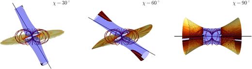
3D rendering of the surface of equilibrium points for χ = 30○, 60○, and 90○, and Γ = 0.9. Unstable part of the surface is shown as transparent blue, stable part as opaque yellow-red with a striped pattern. Dipole magnetic field lines with the outermost radius corresponding to the classical corotation radius are shown with the red lines. The black straight line shows the rotation axis. Position of the camera used for rendering is always at the azimuth of 90○ (while the rotation axis is at the azimuth of 0) and elevation of 10○ above the magnetic equator.
Note that for completely aligned case (χ = 0), equilibrium radius in the plane of the NS equator (α = 90○) becomes (2/3)1/3ω−2/3, which does not coincide with the co-rotation radius ω−2/3. Apparent contradiction is related to the fact that the motions we consider are not free Keplerian motions in the gravity field but instead forced by the kinematic constraints. Corotation radius R = (GM/Ω2)1/3 still remains a characteristic radius scale. However, in the presence of a radiation field, this quantity is altered by a factor (1 − Γ)1/3, that allows to shift the equilibrium points inside the magnetosphere.
2.4 Stability and oscillation frequencies
In Fig. 2, we show several maps of ϰ2 in the θ–φ space. We also mark the points where there are no equilibrium solutions. For an arbitrarily inclined dipole with sin χ ≠ 0, there are always directions where ϰ2 is positive in the equilibrium point. The fraction of such points is about several per cent (up to 12 per cent for an orthogonal rotator). For small magnetic angles, they mostly concentrate in a narrow belt situated between the magnetic equator and the rotational equator, and also in crescent-shaped regions close to the rotation axis on the side of the closest magnetic pole. These secondary stable regions are usually located far away from the NS, but approach at higher χ (see Fig. 1). The maximal possible frequency is about |$\sqrt{3}\omega$|. In Fig. 3, we show how the frequency distribution changes with magnetic angle.
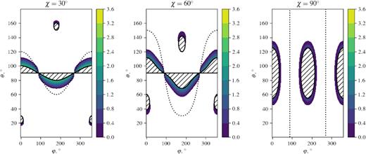
Direction maps for rotating dipoles with χ = 30○, 60○, and 90○. The shaded regions have equilibrium points with positive ϰ2 (colour-coded in ω2 units). The hatched regions have no equilibrium points at all. The dotted curve is the rotational equator (α = π/2).
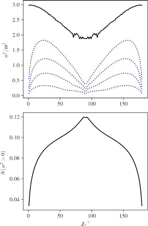
Upper panel: maximal epicyclic frequency squared as a function of magnetic angle. The dotted blue lines are frequency quantiles (0.2, 0.4, 0.6, and 0.8). Lower panel: fraction of the total solid angle where ϰ2 > 0. The solid angle is calculated from the point of view of an observer located at the centre of the NS.
2.5 Negative effective mass
Though one would not expect any astrophysical objects, especially accreting, to have negative masses, strong, compact radiation source situated near the surface of the star may mimic this exotic situation. Real super-Eddington sources, of course, should have finite size, but we so far limit ourselves to a simple, point-source, approximation. Even then, the contribution of the radiation source depends also on the optical depth τ of the test fluid particle: in the optically thin case, violation of the Eddington limit means effectively negative mass, while taking into account the optical depth effects alters the Eddington factor Γ by about a factor of τ, as the same radiation pressure force is now applied to a larger mass. In this case, the sign of equation (10) should change (let us consider the power of 1/3 as a cubic root), but the expression for the oscillation frequency (11) remains valid.
Qualitatively, the spatial distribution of the stable zones remains similar, but now they are confined to the former regions of negative x. The fraction of stable points is smaller, up to 6 per cent (see Fig. 4). As in the positive-mass case, the characteristic frequencies form a broad distribution in the range |$(0-\sqrt{3})\Omega$|.
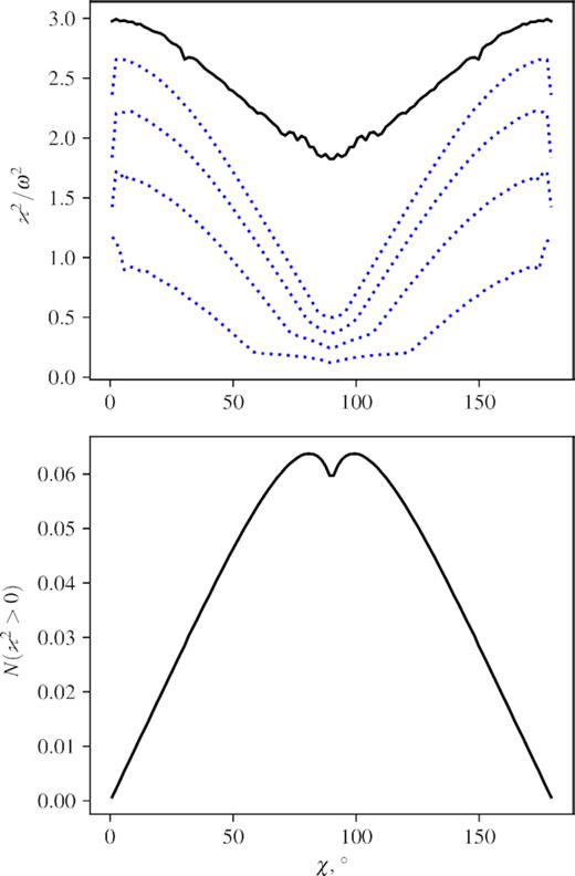
The same as the previous figure, but for the negative effective mass case.
3 DISCUSSION
3.1 Properties of the oscillations
When the inertial oscillations are possible, their frequencies span the range from 0 to a maximal value dependent on χ and changing between approximately |$\sqrt{2}\Omega$| (for an exactly orthogonal dipole, the maximum frequency value is slightly smaller than |$\sqrt{2}$| times spin frequency) and |$\sqrt{3}\Omega$|. Distribution over the frequencies is smooth, with a median value close to Ω. Thus, it is impossible to explain the frequencies larger than a couple of spin frequencies with inertial modes in the approximation we use. Whenever centrifugal force is important, it sets the frequency scale. Hence, independently of the size of the magnetosphere and the contribution of radiation pressure to effective gravity, the characteristic frequencies of the inertial modes are close to the spin and create excess power around the spin frequency. Depending on the oscillation excitation conditions and the presence of matter in the regions of stable equilibrium, the actual variability spectrum may vary, but the distribution of frequencies shown in Fig. 3 suggests roughly constant power up to about (0.5 − 1.0)Ω with a gradual decline at higher frequencies. Such spectral component is harder than the flickering spectrum of the disc with the power roughly inversely proportional to frequency (Lyubarskii 1997), and thus will stand out only near the break.
This picture is similar to the effects observed in some X-ray pulsars in outbursts (see e.g. fig. 2 of Revnivtsev et al. 2009, or Mönkkönen et al. 2019), where the flicker noise becomes contaminated with a peaked (in the sense of f × PDS) component centred at about the break frequency. Though the presence of a peak close to the break frequencies is questionable (the same excess in spectral power may be explained by a harder flicker noise slope), some X-ray pulsars also show quasi-periodic oscillations (QPOs) at frequencies comparable to the break frequency (Angelini, Stella & Parmar 1989; Finger, Wilson & Harmon 1996; Reig & Nespoli 2013). As those features are usually observed during outbursts, and the PDS in quiescence is much flatter, increase in luminosity is apparently an important factor. For an NS close to or exceeding its Eddington limit, the 1 − Γ multiplier in equation (3) is significantly lower than unity, making it possible to reach a force equilibrium inside the magnetosphere without surpassing the propeller limit (Illarionov & Sunyaev 1975), just by decreasing the effective gravity for the optically thin regions.
We suggest that some streams and blobs of accreting matter are at large luminosities trapped in the stable equilibrium points, creating variable reflection and absorption in the observed light curves. An important requirement for the material involved in these motions is its low optical depth to the radiation responsible for the effective antigravity. Large optical depth τ ≫ 1 will effectively decrease Γ by about a factor of τ. The matter trapped near the equilibrium points is not necessarily a part of the accretion flow, and thus can have an optical depth much smaller than the optical depth of the accretion flow itself. The probable origin of the oscillating matter is the same as that of the accretion flow: interchange instabilities effectively load some of the closed magnetic field lines with mass. In general, the magnetosphere is transparent to the thermal radiation of the accretion column (otherwise it would be impossible to observe X-ray pulsars), and some portions of plasma will always suffer the action of a ∝ R−2 radiation force. In Fig. 5, we qualitatively show the flows and equilibrium surfaces of an X-ray pulsar magnetosphere as we see it.
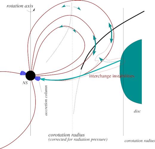
Qualitative scheme illustrating the structure of the magnetosphere and its equilibrium surfaces. Magnetic field lines are shown with the solid red curves. The thick solid black line shows part of the equilibrium surface where the equilibrium points are stable. Each value of Γ corresponds to a surface like this, all its spatial dimensions scaling with the Eddington factor as ∝(1 − Γ)1/3. The blue arrows show the flows of plasma inside the magnetosphere: the main accretion stream (the long single-headed arrow), stable oscillations (the solid teal lines), and unstable points (the dotted teal).
3.2 Observability of the inertial oscillation mode
The easiest way to make the inertial oscillations visible is obscuration of the central source. Even at high, super-Eddington accretion rate, accretion column is much more compact than the size of the magnetosphere, which allows any variation of density to block some part of the emission from the column. Observed fractional variations of the order percents and tens of percents (Revnivtsev et al. 2009) requires comparable optical depths, τ ∼ 0.1 − 1. For this, of course, the optical depth of the variable density component should not be too low: expected relative flux variations are of the order of optical depth.
4 CONCLUSIONS
Motion inside a dipolar magnetosphere has certain equilibrium points, that in some cases (up to 12 per cent of the total solid angle covered by the equilibrium points) are stable. Inertial oscillations in these stable points have frequencies scaling with the spin frequency of the star and roughly homogeneously populating the range from zero to about spin frequency.
Inertial modes in a rotating magnetosphere can not explain the higher frequency noise observed, for instance, in GRO 1744-28, but can account for the varying shape of the PDS near the break frequency observed during the flares of some X-ray pulsars. High luminosity is most likely important as a way to decrease the effective gravity and thus create dynamic equilibrium points inside the magnetosphere.
ACKNOWLEDGEMENTS
We would like to thank Sergey Tsygankov for interesting discussions about the power-density spectra of X-ray pulsars, and the anonymous referee for valuable comments. The 3D plot in this paper was produced with help of mayavi software (Ramachandran & Varoquaux 2011) and Sebastian Mueller’s mlabtex package https://github.com/MuellerSeb/mlabtex. The authors acknowledge the support from the Program of development of the Moscow State University (Leading Scientific School ‘Physics of stars, relativistic objects and galaxies’). AB also thanks for partial support of Russian Government Program of Competitive Growth of Kazan Federal University.
