Improved gravitational radiation time-scales: significance for LISA and LIGO-Virgo sources

Zwick, Lorenz; Capelo, Pedro R; Bortolas, Elisa; Mayer, Lucio; Amaro-Seoane, Pau

doi:10.1093/mnras/staa1314

ABSTRACT

We present a revised version of Peters’ time-scale for the gravitational wave (GW)-induced decay of two point masses. The new formula includes the effects of the first-order post-Newtonian perturbation and additionally provides a simple fit to account for the Newtonian self-consistent evolution of the eccentricity. The revised time-scale is found by multiplying Peters’ estimate by two factors, |$R(e_0)= 8^{1-\sqrt{1-e_0}}$| and Q_f(p₀) = exp (2.5(r_S/p₀)), where e₀ and p₀ are the initial eccentricity and periapsis, respectively, and r_S the Schwarzschild radius of the system. Their use can correct errors of a factor of 1–10 that arise from using the original Peters’ formula. We apply the revised time-scales to a set of typical sources for existing ground-based laser interferometers and for the future Laser Interferometer Space Antenna (LISA), at the onset of their GW-driven decay. We argue that our more accurate model for the orbital evolution will affect current event- and detection-rate estimates for mergers of compact object binaries, with stronger deviations for eccentric LISA sources, such as extreme and intermediate mass-ratio inspirals. We propose the correction factors R and Q_f as a simple prescription to quantify decay time-scales more accurately in future population synthesis models. We also suggest that the corrected time-scale may be used as a computationally efficient alternative to numerical integration in other applications that include the modelling of radiation reaction for eccentric sources.

black hole physics, gravitational waves, methods: analytical

1 INTRODUCTION

The era of gravitational-wave (GW) astronomy started with the detection of merging stellar-mass black holes (BHs) and inspiralling neutron stars by the ground-based Laser Interferometer GW Observatory (LIGO) and Virgo detectors (Abbott et al. 2016; Abbott et al. 2017, 2019). These two detectors, along with the upcoming Laser Interferometer Space Antenna (LISA; Amaro-Seoane et al. 2017; Barack et al. 2019), not only allow physicists to observe the Universe, but also offer an incredible tool to actively test the current theory of gravity, general relativity (GR). Making a prediction for a gravitational signal requires precise modelling of the physics of the source. Since the first successful numerical integration of the evolution of binary BH space–time (Pretorius 2005), we have been in the position of simulating relativistic mergers in GR. The required integration is, however, extremely demanding for current computational resources, which makes covering a substantial part of the source’s parameter space by means of fully relativistic simulations impractical. Moreover, different types of GW sources interact very differently with their astrophysical surroundings (see, e.g. Barausse, Cardoso & Pani 2014). These interactions must be modelled in order to produce realistic event- and detection-rate estimates. Fortunately, there have been major developments in the field of approximations to GR, which allow to model both the sources and their surroundings more efficiently than a fully relativistic simulation. Schemes such as the post-Newtonian (PN) expansion (see, e.g. Blanchet 2014) or the effective one-body approach (see, e.g. Damour & Nagar 2016) are used to find approximate solutions of Einstein’s field equations and the associated equations of motion for the compact-object binary. They successfully describe the relevant features of fully relativistic orbits, such as perihelion precession and radiation of GWs, and can be used to cover a larger amount of parameter space at the loss of some precision. The latter process is especially relevant, as it determines how relativistic orbits shrink as they lose energy due to gravitational radiation.

The first successful quantitative description of the evolution of a binary’s orbit by means of GW induced decay is due to Peters (1964), who used the quadrupole formula to calculate how the semimajor axis and the eccentricity of a Keplerian ellipse evolve in time. By taking these evolution equations, it is possible to find an approximate analytical estimate of the time-scale to the eventual binary’s coalescence, if one does not take into account the self-consistent evolution of the eccentricity. This expression, commonly known as ‘Peters’ formula’ or ‘Peters’ time-scale’, is exact for circular orbits and progressively less accurate for more eccentric ones. When a direct integration of the evolution equations is too computationally expensive, Peters’ time-scale shines for its simplicity and predictive power, and is used in a wide range of applications to model the GW induced decay of various kinds of binary orbits (see, e.g. Farris et al. 2015; VanLandingham et al. 2016; Amaro-Seoane 2018; Bortolas & Mapelli 2019, and many others). At the present time, however, GW detectors such as LIGO/Virgo (and, in the future, LISA) are potentially able to probe eccentric orbits, for which Peters’ formula is less accurate. Many GW sources are expected to radiate while retaining medium (e ≳ 0.5) to very high (e ≳ 0.9) eccentricities (e.g. Amaro-Seoane et al. 2007b; Antonini & Rasio 2016; Bonetti et al. 2016, 2018; Khan et al. 2018; Bonetti et al. 2019; Giacobbo & Mapelli 2019b, a). Furthermore, the Newtonian analysis carried out by Peters (1964) is expected to fail for sources that will complete many GW cycles in strong-gravity regimes. In this paper, we address these issues and revise Peters’ formula to make it more adequate to tackle these more extreme types of sources.

In Section 2, we present the theoretical background of the problem, focussing on the PN series and the parametrization of relativistic orbits. In Section 3, we derive and discuss an analytical PN correction to Peters’ time-scale. We then address the problem of the self-consistent evolution of the eccentricity, as well as calibrate the analytical correction with more complete numerical calculations. In Section 4, we discuss our findings and give a few examples for the most interesting sources of GWs, i.e. binaries of supermassive BHs (SMBHs), binaries of stellar-mass BHs, and extreme and intermediate mass-ratio inspirals (EMRIs and IMRIs). We speculate on the effects of the correction on event-rate estimates for GW detectors such as LIGO-Virgo and LISA.

2 THEORETICAL BACKGROUND

In order to analytically describe the motion of two bodies in GR, it is necessary to approximate Einstein’s field equations. An important and powerful approximation scheme is the Arnowitt–Deser–Misner formalism (hereafter ADM; Arnowitt, Deser & Misner 1959; see also Arnowitt, Deser & Misner 2008). It offers a way to describe the motion of a binary system through the familiar concept of a Hamiltonian and Hamilton’s equations for the separation and momentum vectors of the bodies. The ADM Hamiltonian, H_ADM, is organized into a PN series. Here the PN order is denoted with the index H_i and H_N denotes the Newtonian contribution:

$$\begin{eqnarray*} H_{\rm ADM} = H_{\rm N} + \frac{1}{c^2}H_{1} + \frac{1}{c^4}H_{2} + \frac{1}{c^5}H_{2.5}(t) + \frac{1}{c^6}H_{3} + \cdots, \end{eqnarray*}$$

(1)

where c is the speed of light in vacuum. Different gravitational effects (such as precession, spin-orbit coupling, etc.; see Schäfer & Jaranowski 2018 and references therein) enter the picture at their respective PN orders. Whereas all orders depend on the canonical variables, the 2.5 and all subsequent half-integer orders also explicitly depend on time. This is because half-integer orders describe energy dissipation due to GWs. The 2.5-term of the ADM Hamiltonian is determined by the quadrupole moment tensor of a Newtonian ellipse |$\boldsymbol {N}$|⁠:

$$\begin{eqnarray*} \frac{{\rm d}H_{2.5}(t)}{{\rm d}t} = \frac{G}{5 c^5}\frac{{\rm d}^3\boldsymbol {N}}{{\rm d}t^3}\frac{{\rm d}^3\boldsymbol {N}}{{\rm d}t^3}, \end{eqnarray*}$$

(2)

where G is the gravitational constant. The explicit time dependence on the half-integer terms of the ADM Hamiltonian precludes the existence of a general analytic solution to Hamilton’s equations. The integer-order part of the ADM Hamiltonian is often called the ‘conservative part’ because it admits the definition of a conserved reduced (i.e. per unit mass) energy E and, in certain cases (e.g. when the spin is zero), even a conserved reduced angular momentum h (Schäfer & Jaranowski 2018).¹ These conserved quantities have been used in Damour & Deruelle (1985), Wex (1995), and, finally, in Memmesheimer, Gopakumar & Schäfer (2004) to produce parametric solutions to the PN Hamilton’s equations that are exact up to third order for binaries with no spin (for another approach, see, e.g. Boetzel et al. 2017). The solutions describe elliptical orbits undergoing periapsis precession; a simple way to describe them is to use the familiar concepts of semimajor axis, a, and eccentricity, e. However, some care is needed because the simple Newtonian relations between energy, angular momentum, and the orbital parameters are no longer valid in the PN model. Rather, the definitions of the orbital parameters are now given as PN series:

$$\begin{eqnarray*} a = -\frac{G M}{2 E} + \frac{a_{\rm 1\, PN}(E,h)}{c^2} + \frac{a_{\rm 2\, PN}(E,h)}{c^4} + \cdots, \end{eqnarray*}$$

(3)

$$\begin{eqnarray*} e^2 = 1 + E h^2 + \frac{e^2_{\rm 1\, PN}(E,h)}{c^2} + \frac{e^2_{\rm 2\, PN}(E,h)}{c^4} + \cdots, \end{eqnarray*}$$

(4)

where M = m₁ + m₂ (with m₁ ≥ m₂) is the combined mass of the two bodies. These orbital parameters (along with the periapsis precession) can be used to describe the third-order PN behaviour of the orbit in the absence of the dissipative gravitational radiation term (2.5 PN). There is, however, a way to reintroduce dissipation effects in the description of the orbit. To understand it, we briefly return to the case of a Newtonian orbit.

The energy E and angular momentum h are conserved quantities of a Newtonian binary orbit. They completely determine its shape and size by means of the following formulas:

$$\begin{eqnarray*} a = -\frac{G M}{2 E}, \end{eqnarray*}$$

(5)

$$\begin{eqnarray*} e^2 = 1 + 2h^2E. \end{eqnarray*}$$

(6)

On the other hand, Einstein’s quadrupole formula (Einstein 1916) predicts that the (non-reduced) energy |$\mathcal {E}$| and angular momentum L will be radiated from a gravitational system in the form of GWs:

$$\begin{eqnarray*} \frac{{\rm d}\mathcal {E}}{{\rm d}t}=\frac{G}{5c^5}\frac{{\rm d}^3M_{ij}}{{\rm d}t^3}\frac{{\rm d}^3M_{ij}}{{\rm d}t^3}, \end{eqnarray*}$$

(7)

$$\begin{eqnarray*} \frac{{\rm d}L}{{\rm d}t}= \epsilon _{zab}\frac{{\rm d}^2M_{ac}}{{\rm d}t^2}\frac{{\rm d}^3M_{bc}}{{\rm d}t^3}. \end{eqnarray*}$$

(8)

Here the matrix |$\boldsymbol {M}$| contains the components of the mass quadrupole moment tensor of the binary for an angular momentum pointing in the z-direction. There is a clear inconsistency between the conserved quantities of a purely Newtonian description and the dissipation equations of the quadrupole formula. This inconsistency can be alleviated by noting that changes in |$\mathcal {E}$| and L occur on time-scales much longer than the typical orbital (radial) period. Indeed, the time-scale over which the (non-reduced) energy changes scales as |${\rm d}t \propto c^5 d\mathcal {E}$|⁠, whereas the typical orbital period is independent of c. This consideration is what allowed Peters (1964) to combine Keplerian celestial mechanics with the quadrupole formula to obtain the equations for the GW-induced evolution of orbital parameters:

$$\begin{eqnarray*} \frac{{\rm d}a}{{\rm d}t} = - \frac{64}{5c^5}\frac{G^3M^3 q}{a^3(1 + q)^2} f(e), \end{eqnarray*}$$

(9)

$$\begin{eqnarray*} \frac{{\rm d}e}{{\rm d}t} = -e\frac{304}{15c^5}\frac{G^3M^3 q}{a^4(1-e^2)^{5/2}(1 + q)^2}\left(1 + \frac{121}{304}e^2\right), \end{eqnarray*}$$

(10)

where

$$\begin{eqnarray*} f(e)= \left(1 + \frac{73}{24}e^2 +\frac{37}{96}e^4\right)(1-e^2)^{-7/2} \end{eqnarray*}$$

(11)

and q = m₂/m₁ ≤ 1 is the mass ratio. These equations describe how a Newtonian orbit slowly changes shape if its energy and angular momentum are radiated away according to the quadrupole formula. By manipulating equations (9) and (10), while also assuming that the eccentricity remains fixed at its initial value, it is possible to find an analytic expression for the time-scale, t_P, over which the orbit decays. The resulting expression is known as ‘Peters’ time-scale’ in the literature. It scales with the fourth power of the initial Keplerian semimajor axis, a₀, weighted by the ‘eccentricity enhancement function’ f(e₀), e₀ being the initial Keplerian eccentricity:

$$\begin{eqnarray*} t_{\rm P} = \frac{5c^5(1 + q)^2}{256 G^3 M^3q} \frac{a_0^4}{f(e_0)}. \end{eqnarray*}$$

(12)

The assumption used in Peters (1964) is that, despite the radiation of energy, the binary is still moving along the orbit predicted by Newtonian mechanics. Note, however, that the results of the quadrupole formula (equation 7) in the context of Peters’ work and the 2.5 PN Hamiltonian term (equation 2) in the context of the ADM formalism are identical. Indeed, there are no additional terms in the ADM Hamiltonian that describe energy radiation before the 3.5 PN order. This suggests that the quadrupole formula should be able to describe the orbital evolution not only of a Newtonian orbit, but also of a PN orbit up to third order.

To prove this statement, one can attempt to ‘improve’ the results of the quadrupole formula. We start with a simple Newtonian orbit and insert it in equation (7). We then obtain an evolution equation for the energy E that scales with c⁻⁵. As noted before, this is already equivalent to the 2.5 PN ADM Hamiltonian. From here on, there are only two possibilities to improve the accuracy of the description of energy radiation via GWs: the contribution of a 1 PN perturbed orbit to quadrupolar radiation and the contribution of a Newtonian orbit to octupolar radiation. To improve it even further, it is necessary to add more and more contributions (see, e.g. Thorne 1980; Galley & Leibovich 2012; Blanchet 2014, for more details on this topic). We show the process in a schematic form:

$$\begin{eqnarray*} \frac{{\rm d}E}{{\rm d}t} &=& 2^2\text{pole[Newton] + first tail contribution} \nonumber \\ &&+ (2^2\text{pole[1~PN]} + 2^3\text{pole[Newton])} \nonumber \\ &&+ (2^2\text{pole[2~PN]} + 2^3\text{pole[1~PN]} + 2^4\text{pole[Newton])} \nonumber \\ &&+ \text{higher order terms}, \end{eqnarray*}$$

(13)

where we denote the operation of calculating the 2ⁿpole contribution of an orbit with the functions ‘2ⁿpole[ ]’. The functions scale with c^{−1 − 2n}. We also denote the various perturbations to the orbital dynamics as ‘Newton, 1 PN, 2 PN, ..., n PN’. The perturbations scale as c⁻²ⁿ. The first tail contribution describes the coupling between the mass quadrupole and the mass monopole and is of one and a half orders higher than the purely quadrupolar radiation. Note how any improvement to the results of the quadrupole formula will necessarily have at least a c⁻⁷ factor. Indeed, any improvement to the quadrupole formula is of 3.5 PN order. The situation is very different if we consider the assumption of Keplerian orbits: Perturbations already arise at the first PN order. Another way to state this is the following: the assumption of Keplerian orbits fails at a lower PN order than the assumption of quadrupolar energy radiation.

The idea of this paper is thus to apply the quadrupole formula to the energy of a PN orbit rather than a Keplerian orbit. The parametric solution to the conservative ADM Hamiltonian equations explicitly depends on some kind of conserved energy and angular momentum, analogous but not necessarily equal to their Newtonian counterparts. By taking these quantities and using them as initial conditions for the energy dissipation equations, we can improve the results derived in Peters (1964) without needing any higher order energy flux term. We are aware that truncating the ADM Hamiltonian at 2.5 PN order is a simplification, as tail effects and 3.5 PN terms in the energy flux are considered to be of ‘relative first order’ with respect to the quadrupole formula. If included, they would contribute to the secular evolution of the 1 PN semimajor axis and eccentricity. However, the truncation at 2.5 PN is justified in the formal sense of a Taylor expansion of the ADM Hamiltonian. From this point of view, the higher order contributions can be interpreted as being small corrections to the overall behaviour of the PN orbital parameters, which is dictated by the quadrupole formula alone (up to order 3 PN included). At the cost of some precision, this simplification (among others) will be absolutely necessary to find an analytic correction to Peters’ formula, valid for a large region of parameter space.

In Sections 3.1 and 3.2, we compute how much these considerations alter the original prediction of Peters (1964) for the duration of a binary decay and discuss the analytic results. In Section 3.4, we perform a numerical analysis of the effect of the 3.5 PN fluxes and re-calibrate the analytical formula to account for them.

3 DERIVATION OF THE CORRECTIONS

3.1 Orbits with identical initial shape

The goal of this section is to derive an explicit analytic correction to Peters’ time-scale in the PN framework. In order for the correction to be analytic, we have to restrict our calculations to the lowest significant order, effectively combining the c⁻² conservative information with the c⁻⁵ non-conservative information.

In their original Newtonian form, equations (9)–(10) simultaneously describe the change of the geometry and that of the energy state of a binary system. The introduction of PN effects breaks this symmetry, and it becomes necessary to carefully compare appropriate initial conditions. In the typically adopted expression for Peters’ time-scale, one usually computes the orbital decay time by plugging in an initial (Keplerian) semimajor axis and eccentricity. Hence, we will express our correction in the same terms.

We start by recalling the explicit first-order expressions for the semimajor axis, a₁, and eccentricity, e₁, of the perturbed orbit (that describe a more realistic orbital shape, i.e. closer to the relativistic result), in terms of the PN conserved energy E₁ and angular momentum h₁ (Memmesheimer et al. 2004):

$$\begin{eqnarray*} a_1 = -\frac{G M}{2 E_1}-\frac{G M \left(7 q ^2+13 q +7\right)}{4 c^2 (1+q)^2}, \end{eqnarray*}$$

(14)

$$\begin{eqnarray*} e_{1}^2 &=& 1+ 2 E_{1} h_{1}^2 \nonumber \\ &&+ \frac{E_1\left(5 E_1 h_1^2 \left(3 q^2+5 q +3\right)+2 \left(6 q ^2+11 q +6\right)\right)}{c^2 (1+q)^2}. \end{eqnarray*}$$

(15)

We want to investigate the difference in the decay time-scale when we compare Newtonian and PN orbits with the same initial ‘shape’. This amounts to setting the perturbed orbital parameters a₁ and e₁ equal to the Newtonian ones, a_N and e_N. In the case of a first-order PN analysis, the equations that one obtains are

$$\begin{eqnarray*} a_1 \overset{!}{=} a_{\rm N}, \end{eqnarray*}$$

(16)

$$\begin{eqnarray*} e_1^2 \overset{!}{=} e_{\rm N}^2. \end{eqnarray*}$$

(17)

By rearranging these expressions, we obtain a set of conditions for the PN energy, E₁, and the PN angular momentum, h₁. We can interpret the resulting conditions as the values that E₁ and h₁ must have in order for the perturbed orbit to be identical to a Newtonian orbit with semimajor axis a_N and eccentricity e_N. The conditions read

$$\begin{eqnarray*} E_1=-\frac{G M}{2 a_{\rm N}}+\frac{G^2 M^2 \left(7 q ^2+13 q +7\right)}{8 a_{\rm N}^2 c^2 (q +1)^2}+O\left(\frac{1}{c^3}\right), \end{eqnarray*}$$

(18)

$$\begin{eqnarray*} h_1^2&=& \frac{a_{\rm N}(1- e_{\rm N}^2)}{G M} \nonumber \\ &&+ \frac{4(q +1)^2+e_{\rm N}^2 \left(2 q ^2+3 q +2\right)}{c^2(q +1)^2}+O\left(\frac{1}{c^3}\right). \end{eqnarray*}$$

(19)

Equations (18) and (19) show that the perturbed orbit has a slightly larger energy and squared angular momentum than the non-perturbed one. In other words, it takes more energy and more angular momentum to sustain a certain shape in a PN gravity field rather than in a Newtonian gravity field. Since excess energy and momentum take time to be radiated away, we come to a qualitative result: PN orbits decay more slowly than what Peters’ formula predicts, when comparing binaries with identical initial shape (i.e. semimajor axis and eccentricity).

This result might seem counter to the common expectation that PN effects reduce the time-scale of the GW-induced decay. This apparent discrepancy is due to the fact that a more common way to confront Newtonian and PN results is to compare orbits with identical initial energy and angular momentum (e.g. Blanchet 2014), and not identical initial semimajor axis and eccentricity. As soon as one includes PN contributions, comparing orbits with the same initial shape or energy and angular momentum is not equivalent any longer. In Appendix A, we show the same analysis for the latter comparison, which indeed produces different results. To quantify the time-scale for the decay, it is useful to define two new parameters, an effective semimajor axis, a_eff, and an effective eccentricity, e_eff:

$$\begin{eqnarray*} a_{\rm eff} =- \frac{G M}{2 E_1}, \end{eqnarray*}$$

(20)

$$\begin{eqnarray*} e_{\rm eff}^2 = 1 + 2 h_1^2 E_1. \end{eqnarray*}$$

(21)

These ‘effective’ parameters are used to construct a fictitious Newtonian orbit that contains all the information regarding the perturbed orbital parameters. Their explicit formulas are

$$\begin{eqnarray*} a_{\rm eff} = a_{\rm N}+ \frac{G M \left(7 q ^2+13 q +7\right)}{4 c^2 (q +1)^2}, \end{eqnarray*}$$

(22)

$$\begin{eqnarray*} e_{\rm eff}^2 &=& e_{\rm N}^2 \nonumber \\ &&- \frac{G M \left(5 e_{\rm N}^2 \left(3 q ^2+5 q +3 \right)+9 q ^2+19 q +9\right)}{4 c^2 a_{\rm N} (q +1)^2}. \end{eqnarray*}$$

(23)

Note that these effective quantities do not carry information on the actual shape of the orbit; we introduce them as convenient variables for the analysis. Equations (23) and (22) imply that (i) the slight increase of the perturbed energy E₁ with respect to the Newtonian energy causes the effective semimajor axis to be larger than the actual one; (ii) the slight increase of the perturbed squared angular momentum |$h_1^2$| causes the squared effective eccentricity to decrease; and (iii) the squared effective eccentricity may, in principle, become negative (indeed, it is always negative if the physical orbit is circular).

Summing up, the effective ellipse is larger and more circular than the actual (PN) orbit because it is constructed using the larger PN energy and angular momentum. However, we incur into a problem if the physical orbit is already very circular. The crucial point is that PN orbits may have more angular momentum than what the classical definition of eccentricity and semimajor axis allow for a given energy. In other words, if the physical orbital eccentricity is smaller than a critical value e_c, no Newtonian orbit exists with corresponding energy and angular momentum, as implied by the possible appearance of a negative ‘squared eccentricity’. In Fig. 1, we show the effective versus the Newtonian eccentricity for orbits with different initial sizes. There exists, however, a simple solution to this apparent inconsistency, which extends the validity of the effective orbit construction to all possible perturbed orbits. Note that, if negative, the absolute value of the squared effective eccentricity is always at least smaller than a 1 PN term:

$$\begin{eqnarray*} \vert e_{\rm eff}^2 \vert = \left| e_{\rm N}^2 - \frac{G M \left(9 + 15 e_{\rm N}^2 \right) }{4 c^2 a_{\rm N}} +O\left(q\right) \right| \lt \left| \frac{6 G M}{ c^2 a_{\rm N}} \right|. \end{eqnarray*}$$

(24)

Therefore, if we allow for a small adjustment (smaller than a 1 PN term) to the squared angular momentum of the effective ellipse, we can neglect the cases where the squared effective eccentricity would be negative and instead treat the effective ellipse as having zero eccentricity.

Figure 1.

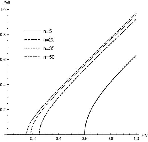
We plot the effective eccentricity (equation 23) against the Newtonian eccentricity for orbits with different initial sizes (a_N = nr_S). The effective eccentricity is always slightly smaller than its Newtonian counterpart. The significance of this difference is determined by the orbit’s distance to the Schwarzschild radius of the system: it decreases for larger orbits, as expected for any PN perturbation. In very strong gravity regimes, there is no way to describe the energy and angular momentum of the orbit as an effective Newtonian ellipse. In the plot, we see this effect when the effective eccentricity becomes zero.

Open in new tab Download slide

The time-scale for the orbit’s decay can now be computed by integrating equation (9) from the value a_eff to a value representing the coalescence of the binary, which we simply take to be the effective Schwarzschild radius of the two-body system (hereafter, simply Schwarzschild radius), r_S = 2GMc⁻².

In order to solve the decay equation (9) analytically, we have to make the simplifying assumption of small initial eccentricity (⁠|$e_{\rm N}^2 \approx 0$|⁠). For a given initial semimajor axis a₀, the time evolution of a circular orbit reads

$$\begin{eqnarray*} a_{\rm N}(t)= \sqrt{2} \left(a_0^4-\frac{256 G^3 M^3 q t}{5 c^5 (q +1)^2}\right)^{{1}/{4}}. \end{eqnarray*}$$

(25)

With this formula, we can compute the corrected time-scale, τ_c, for the GW decay of a perturbed orbit by replacing the initial semimajor axis a₀ with the effective semimajor axis, and subsequently solving equation (25) for t. The resulting expression would only be valid for circular orbits. Nonetheless, there is a simple way to reintroduce large initial eccentricities. Note that, since the time-scale scales with the fourth power of a₀, most of the decay time is spent in the neighbourhood of the initial conditions. Therefore, we can adjust the corrected time-scale by dividing it by the eccentricity enhancement function f(e) evaluated at the initial effective eccentricity:

$$\begin{eqnarray*} \tau _{\rm c} \rightarrow \frac{\tau _{\rm c}}{f(e_{\text{eff}})}. \end{eqnarray*}$$

(26)

This manipulation is essentially the same one that is used in Peters (1964) to yield what we refer to in this paper as Peters’ formula (equation 12).

The results of the calculations are most readable when expressed in terms of multiples a₀ = nr_S of the Schwarzschild radius:

$$\begin{eqnarray*} \tau _{\rm c}=\frac{5 (q +1)^2 \left(\left(n+\frac{7 q ^2+13 q +7}{8 (q +1)^2}\right)^4-\frac{1}{4}\right)r_{\rm S}}{32 c q f(e_{\rm eff}) }. \end{eqnarray*}$$

(27)

We report the ratio ν_g = τ_c/t_P and difference δ_g = τ_c − t_P between time-scales in the two limiting cases of q → 0,

$$\begin{eqnarray*} \nu _{\rm g} =\frac{4 \left(n+\frac{7}{8}\right)^4-1}{4 n^4-1} \frac{f(e_0)}{f(e_{\rm eff})} \ge 1, \end{eqnarray*}$$

(28)

$$\begin{eqnarray*} \delta _{\rm g} =\frac{5 r_{\rm S} }{32 c q }\left(\frac{ \left(n+\frac{7}{8}\right)^4}{f(e_{\rm eff})} - \frac{ n^4}{f(e_{0})} \right) \ge 0, \end{eqnarray*}$$

(29)

and q → 1,

$$\begin{eqnarray*} \nu _{\rm g} =\frac{4 \left(n+\frac{27}{32}\right)^4-1}{4 n^4-1} \frac{f(e_0)}{f(e_{\rm eff})} \ge 1, \end{eqnarray*}$$

(30)

$$\begin{eqnarray*} \delta _{\rm g} =\frac{5 r_{\rm S} }{32 c }\left(\frac{4 n^4-\frac{12\,117\,361}{1048\,576}}{f(e_{\rm eff})} - \frac{4 n^4-1}{f(e_{0})} \right) \ge 0, \end{eqnarray*}$$

(31)

computed for the same initial orbital shapes.

3.2 Simplifying the analytic result

In the previous section, we defined two quantities (ν_g and δ_g) that describe the deviations from Peters’ formula when taking PN perturbations to the orbit into account and comparing orbits with identical initial shape. Now, let us take a closer look at the ratio of the corrected to the standard Peters’ time-scale.

The ratio ν_g approaches unity for n approaching infinity. This is expected because any PN perturbation to the binary orbit has to vanish as we increase the relative distance between the two bodies. However, a quick glance at Fig. 2 shows that, as n increases, the ratio ν_g remains quite large for a wide range of n. More specifically, the behaviour of ν_g (which is also a function of the initial orbital eccentricity) strongly depends on the value of the initial orbital periapsis, p₀ = a₀(1 − e₀): The smaller the periapsis, the more enhanced the deviation from Peters’ time-scale.

Figure 2.

We show the behaviour of the PN correction to Peters’ time-scale ratio ν_g plotted against the initial semimajor axis measured in Schwarzschild radii (a₀ = nr_S). Since the ratio ν_g depends on the orbital eccentricity, we plot it for different values of the initial eccentricity e₀. ν_g approaches unity for n → ∞, as expected, but can still be significantly different from one for very large n if the initial orbit is very eccentric, suggesting that the magnitude of this correction is sensitive to the periapsis of the system.

Open in new tab Download slide

The explicit analytical formula of ν_g is still rather complex. It is possible to find a much simpler formula that can approximate it very well by taking the limit of very large n (large orbits) and e₀ approaching unity (very eccentric orbits):

$$\begin{eqnarray*} \nu _{\rm g} \rightarrow 1+ \frac{7 \left(6 q^2+11 q+6\right)}{8 \left(1-e_0\right) n (q+1)^2}. \end{eqnarray*}$$

(32)

It turns out that the above approximation actually covers most of the phase space without producing a significant loss of precision. This aspect can be appreciated by looking at Fig. 3, which shows the discrepancy between the approximated ν_g (equation 32) and the exact 1 PN value (equation 28). In short, the absolute error of the approximation with respect to the full 1 PN result is of the order of a 2 PN term, and can therefore be neglected.

Figure 3.

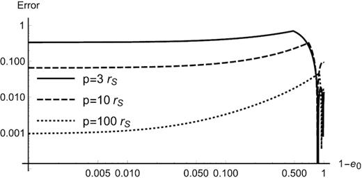
We show the relative error of the simplified ratio Q (equation 34) to the exact first-order correction ν_g (equation 27 divided by t_P), for a wide range of initial conditions. For very eccentric orbits (1 − e₀ < 0.1), the error is of the magnitude of a PN term r_S/p₀, where p₀ is the periapsis. This implies that the absolute error that arises by using this approximation instead of ν_g is as large as a second-order PN term and can be neglected. The relative error increases for orbits with intermediate eccentricity (1 − e₀ ≈ 0.5) but dramatically falls for almost circular orbits (1 − e₀ ≈ 0.8). It also shows a complicated behaviour for very low eccentricities but always remains small.

Open in new tab Download slide

We can rewrite equation (32) as

$$\begin{eqnarray*} \nu _{\rm g} = 1 +\frac{7 \left(6 q^2+11 q+6\right) r_{\rm S}}{8 \left(1-e_0\right) a_0 (q+1)^2} = 1+K(q) \frac{r_{\rm S}}{a_0(1-e_0)} \ge 1. \end{eqnarray*}$$

(33)

The PN-correction factor can be easily interpreted: it shows that the time-scale of gravitational decay is affected in a significant way by PN perturbations if the orbital periapsis p comes close to the Schwarzschild radius of the system. The magnitude of the correction scales as K × (r_S/p₀), with K(q) being a monotonic function of the mass ratio q that decreases from 5.25 (or 21/4) to approximately 5.03 (or 161/32) as q ranges from 0 to 1. The variation is very weak because the first-order perturbations to the semimajor axis and eccentricity only weakly depend on the mass ratio. We therefore name the approximation value for the above ratio the ‘PN correction factor’ Q:

$$\begin{eqnarray*} Q(p_0) = 1+5 \frac{r_{\rm S}}{a_0(1-e_0)} \ge 1. \end{eqnarray*}$$

(34)

By using this simple factor, we can restate the qualitative result of Section 3.1 in a more precise form, valid when comparing orbits with identical initial semimajor axis and eccentricity, within the assumptions of this section: Peters’ time-scale is too short by a factor of Q that is relevant whenever the periapsis p₀of the binary comes close to the Schwarzschild radius r_S. The factor is given by the formula|$Q=1 + 5 r_{\rm S} p_0^{-1}$|⁠.

3.3 Inclusion of the secular evolution of the eccentricity

In the previous sections, we neglected the self-consistent evolution of the eccentricity, in order to keep the method analytical, and used the common practice of dividing the decay time for circular orbits by the eccentricity enhancement function f(e₀). This approximation is known to break down for orbits that start with very high eccentricities and can produce very large errors (of the order of 0, ∼400, and ∼700 per cent for initial eccentricities of 0, 0.9, and 0.999, respectively) in the evaluation of the decay time-scale. It is mostly used as a lower bound estimate for the self-consistently evolved case. Even in a purely Newtonian framework, the only way to achieve more accurate results is to integrate equations (9) and (10) directly and obtain a numerical value for the decay time-scale. While the numerical integration is straightforward and fast on a case-by-case basis, it is much less convenient in applications that require a quick and simple estimate for the decay time-scale of many orbits.

In this section, we present a simple correction to Peters’ formula that extends its validity to highly eccentric orbits in a Newtonian-gravity regime. To find this correction, we have performed numerous fully consistent integrations of equations (9) and (10) to find an accurate decay time-scale. We define the correction factor R as the ratio between such accurate Newtonian time-scales and the lower bound given by Peters’ formula (i.e. equation 12). It turns out that expressing the deviations in this manner cancels out the effects of most of the parameters: There is no appreciable variation in the value of the ratio R when changing the mass ratio, the total mass, or the initial semimajor axis.

A plot of R(e₀) and our proposal for a convenient fitting function are shown in the top panel of Fig. 4. We found a surprisingly performing fitting function of the form |$R(e_0)= A ^{ (1-(1-e_0)^{m})}$|⁠. The best-fitting parameters, when using 50 equally spaced points in log₁₀(e₀) between e₀ = 0 and 0.9999, are A = 8.023 and m = 0.502. The variation in the best-fitting values when choosing different semimajor axes, total masses, or mass ratios is limited to the third decimal place. By using round numbers, and without any great loss of accuracy, we adopt

$$\begin{eqnarray*} R(e_0) = 8^{1-\sqrt{1-e_0}}. \end{eqnarray*}$$

(35)

The bottom panel of Fig. 4 shows the error that arises from using equation (35) with respect to the numerical results. It is clear that the proposed fit is an accurate estimation of the numerical result, especially for eccentric orbits (e₀ ≳ 0.5), where the relative error falls below a few per cent. For the sake of clarity, we stress that we do not claim that this is the best possible fit for the given data as a function of eccentricity. Indeed, for more circular orbits, we incur into some errors of fractional order (≲10 per cent), comparable to the performance of Peters’ formula. However, we can claim that the fitted ratio R(e₀) is sufficiently accurate and simple to extend the validity of Peters’ formula to a wide range of initial eccentricities. The ratio R(e₀) can be thought as an extension of the eccentricity enhancement function. We can thus use the original Peters’ formula (equation 12), after replacing f(e₀) with the ‘effective eccentricity enhancement function’ f(e₀)/R(e₀). The corrected Newtonian formula can be manipulated just as easily as Peters’ formula, can correct errors as large as a factor of eight, and it is equivalent to the integration of the two coupled evolution equations (9) and (10).

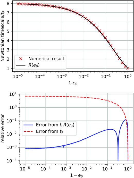
$The top panel shows the ratio of the decay time-scale obtained by integrating the evolution equations (9) and (10) to Peters’ formula (red crosses). The black solid line shows the fitting function $R(e_0)=8^{1-\sqrt{1-e_0}}$. The bottom panel shows the relative error from the numerical result that one incurs into when using Peters’ formula (red dashed line) and when using the corrected formula R(e0)tP (blue solid line). The corrected time-scale reproduces the true result within a few per cent accuracy for a large region of parameter space, whereas Peters’ formula dramatically fails (relative error of order ∼100 per cent) as soon as the eccentricity is larger than ∼0.5.$

Figure 4.

The top panel shows the ratio of the decay time-scale obtained by integrating the evolution equations (9) and (10) to Peters’ formula (red crosses). The black solid line shows the fitting function |$R(e_0)=8^{1-\sqrt{1-e_0}}$|⁠. The bottom panel shows the relative error from the numerical result that one incurs into when using Peters’ formula (red dashed line) and when using the corrected formula R(e₀)t_P (blue solid line). The corrected time-scale reproduces the true result within a few per cent accuracy for a large region of parameter space, whereas Peters’ formula dramatically fails (relative error of order ∼100 per cent) as soon as the eccentricity is larger than ∼0.5.

Open in new tab Download slide

3.4 Calibration of the PN correction with 3.5 PN fluxes

In the derivation of the analytical PN correction factor Q, we treated the 3.5 PN fluxes (which are of first relative order to the Newtonian fluxes) as a negligible correction in the Taylor expansion of the ADM Hamiltonian (equation 1). In this section, we compare the analytical results from Sections 3.1 and 3.2 with a numerical analysis that includes the 3.5 PN fluxes. In order to achieve this, we performed numerous numerical integrations of the full 3.5 PN evolution equations for the orbital parameters (see, e.g. Mikóczi, Forgács & Vasúth 2015) and studied the effect of varying the total mass, mass ratio, and initial orbital parameters. Similarly to before, we express the results as a ratio between time-scales. This time, we divide the result from the full 3.5 PN evolution equations with the result from the full 2.5 PN evolution equations (i.e. integrating equations 9 and 10). As shown in Fig. 5, we find that this ratio strongly depends on both orbital parameters – initial periapsis and eccentricity. The effects of varying total mass and mass ratio are noticeable, but are significantly smaller than our estimation of how much PN tail effects will change the results. Fig. 5 also shows our proposal for a convenient fit to the integrated data. Led by the findings of previous sections, we chose a fitting function of the form Q_f = exp (Cr_S/p₀) and found the best-fitting value C = 2.5, such that

$$\begin{eqnarray*} Q_{\rm f}(p_0) = \exp \left(2.5 \frac{r_{\rm S}}{p_0} \right). \end{eqnarray*}$$

(36)

Similarly to the previous fitting function R, the goal of using the ratio Q_f is not to perfectly reproduce the full first-order results, but rather to be sufficiently precise and simple to extend the validity of Peters’ formula to more relativistic orbits. Furthermore, a quick estimation of the effect of PN tail contributions (as shown by the representative error bars in the top panel of Fig. 5) shows that trying to fit the eccentricity dependence more precisely will not necessarily lead to a better estimation of the true, fully relativistic result. In other words, the simple fitted ratio in equation (36) is accurate within 1 PN precision. It can successfully describe the trend of including PN contributions to the orbital dynamics and to the energy fluxes. It is not by chance that this fitted ratio has a very similar form as the analytical correction factor Q found in Sections 3.1 and 3.2. Indeed, if we perform the PN expansion in the small parameter r_S/p₀,

$$\begin{eqnarray*} Q_{\rm f}(p_0) = \exp \left(2.5 \frac{r_{\rm S}}{p_0} \right) \approx 1+ 2.5\frac{r_{\rm S}}{p_0} + \mathcal {O}(c^{-3}), \end{eqnarray*}$$

(37)

we recover the same functional form of Q = 1 + 5r_S/p₀.

Figure 5.

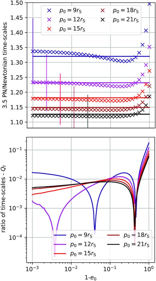
In the top panel, we divide the result from the full 3.5 PN evolution equations by the result from the full 2.5 PN evolution equations (crosses), as a function of initial eccentricity, for different initial periapses. We also show the proposed fits (solid horizontal lines) and a representative uncertainty due to the PN tail perturbations (vertical error bars; see the text for the derivation). In the bottom panel, we plot the relative error that one would incur into by using the fit instead of the true 1 PN result. The errors are well below the typical uncertainty due to the PN tail contributions.

Open in new tab Download slide

Even though the coefficient of the fitted ratio is smaller by a factor of 2, a simple estimate of the effect of PN tail contributions shows that the uncertainties in the coefficients can overlap. We crudely model the effect of PN tail contributions as follows: if the 1 PN correction to the ratio between time-scales is of the form

$$\begin{eqnarray*} 1+D \frac{r_{\rm S}}{p_0}, \end{eqnarray*}$$

(38)

where D is a constant (or a function of eccentricity), then the uncertainty due to the tail correction should be of relative 1.5 PN order. Roughly, we expect it to have the following form:

$$\begin{eqnarray*} 1+D \frac{r_{\rm S}}{p_0} \pm \left(D\frac{r_{\rm S}}{p_0}\right)^{{3}/{2}}, \end{eqnarray*}$$

(39)

which can be expressed as some uncertainty in the coefficient D:

$$\begin{eqnarray*} D \rightarrow D \pm D^{{3}/{2}} \sqrt{\frac{r_{\rm S}}{p_0}}. \end{eqnarray*}$$

(40)

In this estimation, the uncertainties in the coefficients of the ratios Q and Q_f overlap for all orbits with (initial) periapses smaller than approximately 35r_S (where the first PN correction is only ∼10 per cent). In this region of parameter space, both ratios are, in a sense, equivalent and may be used interchangeably. Nonetheless, we believe the fitted ratio Q_f = exp (2.5r_S/p₀) to be more robust than the analytical ratio Q, since it has been produced with more accurate numerical methods. It can be thought of as a ‘calibration’ of the analytical result with the inclusion of the 3.5 PN fluxes. We therefore propose it as a simple way to model the effects of the first-order PN perturbations on the time-scale of the GW-induced decay.

4 DISCUSSION AND CONCLUSIONS

In this work, we introduced the two simple factors R(e₀) and Q_f(a₀, e₀) that, if multiplied by the standard Peters’ formula, can (i) correct for the evolution of the eccentricity and (ii) model the effects of the first-order PN perturbation. The full expression for the corrected Peters’ formula is given in terms of the initial semimajor axis a₀ and eccentricity e₀:

$$\begin{eqnarray*} t_{\rm P}RQ_{\rm f} = \underbrace{ \frac{5c^5(1 + q)^2}{256 G^3 M^3q} \frac{a_0^4}{f(e_0)} }_{\text{Peters' formula}} \underbrace{ 8^{ 1- \sqrt{1-e_0}} \exp \left(\frac{2.5 r_{\rm S}}{a_0(1-e_0)} \right)}_{\text{eccentricity and PN correction}}. \end{eqnarray*}$$

(41)

Fig. 6 shows the interplay between the PN correction and the eccentricity-evolution correction. Even though the former is only a small fraction, the two factors can compound on each other and produce a correction of more than a factor of 10 for very eccentric orbits. This is a clear indication that the standard Peters’ time-scale is an insufficient description of the time-scale of the GW-induced decay for many GW sources.

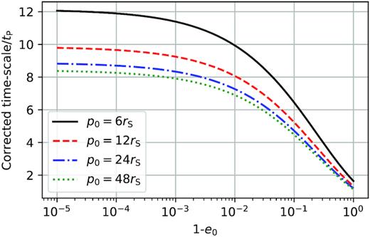
$We show the combination of the correction factors R and Qf as a function of initial eccentricity for different initial periapses. Even though the PN correction is only of fractional order by itself, it can compound with the eccentricity-correction factor for very eccentric orbits. GW sources such as EMRIs are expected to originate from precisely these regions of parameter space (high eccentricity and low periapsis). For such sources, using the corrected Peters’ formula (equation 41) can resolve errors of up to one order of magnitude in the time-scale of GW-induced decay, without needing to resort to numerical integration.$

Figure 6.

We show the combination of the correction factors R and Q_f as a function of initial eccentricity for different initial periapses. Even though the PN correction is only of fractional order by itself, it can compound with the eccentricity-correction factor for very eccentric orbits. GW sources such as EMRIs are expected to originate from precisely these regions of parameter space (high eccentricity and low periapsis). For such sources, using the corrected Peters’ formula (equation 41) can resolve errors of up to one order of magnitude in the time-scale of GW-induced decay, without needing to resort to numerical integration.

Open in new tab Download slide

A useful way to visualise the effects of the correction factors R and Q_f is to compute isochrone curves. This amounts to setting the time-scale of gravitational decay equal to a fixed time τ (i.e. RQ_ft_P = τ or t_P = τ) and, for any given eccentricity, solving for the semimajor axis. We compute the corrected isochrones for the case of an EMRI and plot the results in the (a₀, 1 − e₀) phase space in Fig. 7. The plots would be qualitatively similar for other types of GW sources, such as SMBH binaries and stellar-mass binaries. The effect of the correction factor is to shift the isochrones towards the lower left-hand corner of the phase-space plots. Equivalently, any point in phase space that used to lay on an isochrone labelled by the time t_P (given by Peters’ time-scale) now lays on an isochrone labelled with the corrected time RQ_ft_P.

We show a region of phase space in the initial semimajor axis and eccentricity. The panel shows an EMRI (with m1 = 106 and m2 = 10 M⊙). The plots would be qualitatively similar for other types of GW sources, such as SMBH binaries and stellar-mass binaries. The solid coloured lines represent the isochrone curves (for different τ) obtained with the corrected Peters’ formula (RQftP = τ), whereas the dashed coloured lines are obtained with Peters’ time-scale (tP = τ). The pale, solid couloured lines are computed with only the eccentricity-evolution correction R (i.e. RtP = τ). The black solid curve represents orbits whose periapsis is one Schwarzschild radius.

Figure 7.

We show a region of phase space in the initial semimajor axis and eccentricity. The panel shows an EMRI (with m₁ = 10⁶ and m₂ = 10 M_⊙). The plots would be qualitatively similar for other types of GW sources, such as SMBH binaries and stellar-mass binaries. The solid coloured lines represent the isochrone curves (for different τ) obtained with the corrected Peters’ formula (RQ_ft_P = τ), whereas the dashed coloured lines are obtained with Peters’ time-scale (t_P = τ). The pale, solid couloured lines are computed with only the eccentricity-evolution correction R (i.e. Rt_P = τ). The black solid curve represents orbits whose periapsis is one Schwarzschild radius.

Open in new tab Download slide

It is worth noting that the discrepancy between the corrected and classical Peters’ formula is enhanced for binaries with a large eccentricity. A wide variety of physical processes are known to enhance the eccentricity of a candidate GW source (and thus promote the inspiral) at all mass scales. For instance, the eccentricity of stellar compact binaries may increase as a result of the supernova kicks experienced by stellar BHs and neutron stars at birth (Giacobbo & Mapelli 2019a,b); in addition, evolution in triplets can induce large eccentricities due to Kozai–Lidov (Kozai 1962; Lidov 1962) cycles and chaotic evolution for both stellar (e.g. Antonini & Rasio 2016; Bonetti et al. 2018) and SMBH binaries (e.g. Bonetti et al. 2016). As a notable example, Bonetti et al. (2019) showed that evolution in triplets can produce SMBH binaries whose eccentricity is greater than 0.9 when the source enters the LISA band. Finally, most EMRIs are expected to enter the GW phase via the classical two-body relaxation channel (Hils & Bender 1995; Sigurdsson 1997) with eccentricities very close to unity (Amaro-Seoane et al. 2007b). For these reasons, we claim that the correction factors for Peters’ time-scale will have an effect on the predicted detection rates of the LIGO-Virgo and LISA observatories. Peters’ time-scale is commonly used to estimate the likelihood of a population of compact objects to produce gravitational signals detectable by GW observatories. It is used both in the modelling of the astrophysics (O’Leary, Kocsis & Loeb 2009; Barausse 2012) and in signal analysis (Klein et al. 2016). A fractional increase in the time-scale of gravitational decay corresponds to a fractional increase in the time that any signal remains in the optimal frequency band of the observatory. Moreover, it will have some astrophysical implication on the rates at which sources of GWs are produced. The interplay between these two effects will affect how many and what potential sources of GWs are considered promising for both LISA and LIGO-Virgo observatories. We are currently working on a quantitative formulation of this effect, with a focus on the upcoming detector LISA. Preliminary calculations show that it might increase the predicted rates because of the better signal-to-noise ratios arising from longer decay durations. However, this effect must be weighted against other astrophysical implications of an increased GW time-scale.

As opposed to the correction factors Q_f and R, the absolute difference between Peters’ and the corrected time-scale strongly depends on the mass ratio and total mass of the system. For the special case of EMRIs, mere fractional corrections to the GW time-scale can be of the order of astrophysical time-scales describing other dynamical processes around a SMBH. The correction factors Q_f and R might therefore have significant astrophysical implications. Most EMRIs are believed to be generated by the scattering of a stellar-mass compact object to an orbit with very low angular momentum (Hils & Bender 1995; Sigurdsson 1997) via the two-body relaxation process. However, two-body scatterings can also deflect the orbit of an inspiral before it has had time to complete its gravitational decay. In order to understand whether a compact object reaches its GW-induced coalescence, one has to compare the time-scale of gravitational decay to the two-body relaxation time-scale, given by

$$\begin{eqnarray*} t_{\rm r} = \frac{\sqrt{18 \pi ^4}}{32 C_{\gamma }}\left(\frac{G M_{\rm SMBH}}{ a}\right)^{3/2}\frac{(1-e^2)a^{\gamma }}{G^2 m_{\rm s} m_{\rm o} N \ln (\frac{M_{\rm SMBH}}{2 m_{\rm s}})}, \end{eqnarray*}$$

(42)

where M_SMBH = 4.3 × 10⁶ M_⊙ is the SMBH mass, m_s = 1 M_⊙ is the mass of a typical field star, m_o = 10 M_⊙ is the mass of the compact object undergoing the process, N = 10⁶ is the number of stars in a given unit sphere of radius of 1 pc, γ is the exponent of the number density profile, and C_γ is a constant of order unity. The values of the parameters introduced above are chosen to represent the relaxation process in a Milky Way analogue (see, e.g. Bortolas & Mapelli 2019).

In Fig. 8, we plot the curves that equate the two-body relaxation time-scale to the time-scale of gravitational decay for different power-law stellar distributions, solving t_P = t_r or RQ_ft_P = t_r for the semimajor axis, for a given eccentricity (Amaro-Seoane et al. 2007a; Merritt et al. 2011; Bortolas & Mapelli 2019). In very rough terms, objects that fall above such curves in (a₀, 1 − e₀) phase space are unlikely to undergo an EMRI as their orbit will be likely scattered in a ‘safer’ zone by two-body relaxation.

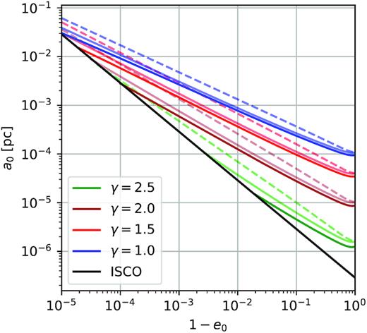
We show a region of phase space in the initial semimajor axis and eccentricity, for an EMRI system with m1 = 4.3 × 106 and m2 = 10 M⊙. The black solid line represents the effective innermost stable circular orbit (ISCO; 3rS), whereas the coloured solid (dashed) lines are the curves obtained by equating the two-body relaxation time-scale to the corrected (uncorrected) Peters’ time-scale, for four different density power laws (γ = 1; 1.5; 2; 2.5). The pale, solid coloured lines are computed by only taking into account the eccentricity-evolution correction R (RtP = tr). Note how the corrected lines (RQftP = tr) diverge from the uncorrected ones (tP = tr) for eccentric orbits, where the PN correction compounds with the eccentricity-evolution correction. Orbits below the ISCO line are expected to decay too quickly to produce easily detectable GW signals and are therefore not relevant. Similarly, orbits above the coloured lines are scattered before gravitational radiation has time to significantly affect their orbit. This leaves us with the phase-space volume between the black and coloured lines as a proxy of the region of potential EMRI candidates. Such volume is drastically reduced by the correction(s) to Peters’ time-scale.

Figure 8.

We show a region of phase space in the initial semimajor axis and eccentricity, for an EMRI system with m₁ = 4.3 × 10⁶ and m₂ = 10 M_⊙. The black solid line represents the effective innermost stable circular orbit (ISCO; 3r_S), whereas the coloured solid (dashed) lines are the curves obtained by equating the two-body relaxation time-scale to the corrected (uncorrected) Peters’ time-scale, for four different density power laws (γ = 1; 1.5; 2; 2.5). The pale, solid coloured lines are computed by only taking into account the eccentricity-evolution correction R (Rt_P = t_r). Note how the corrected lines (RQ_ft_P = t_r) diverge from the uncorrected ones (t_P = t_r) for eccentric orbits, where the PN correction compounds with the eccentricity-evolution correction. Orbits below the ISCO line are expected to decay too quickly to produce easily detectable GW signals and are therefore not relevant. Similarly, orbits above the coloured lines are scattered before gravitational radiation has time to significantly affect their orbit. This leaves us with the phase-space volume between the black and coloured lines as a proxy of the region of potential EMRI candidates. Such volume is drastically reduced by the correction(s) to Peters’ time-scale.

Open in new tab Download slide

The effect of the correction factors is again to shift the curves towards the lower left-hand corner of the phase-space plots. This means that slices of parameter space that would have previously been considered promising for EMRIs are now removed. For very steep power laws (i.e. γ = 2; 2.5), the effect of the PN correction is very noticeable even for low-eccentricity orbits. Steep density profiles could be produced by the effect of strong mass segregation (Alexander & Hopman 2009; Preto & Amaro-Seoane 2010) aided by the slow natal kicks received by stellar BHs at birth (Bortolas, Mapelli & Spera 2017). For shallower power laws (i.e. γ = 1; 1.5) expected in the case of weak mass segregation (Bahcall & Wolf 1976, 1977), the shift is significant for eccentric orbits. Even though preliminary, these plots suggest that the correction factors Q_f and R will have a direct effect on previously computed event rates for EMRIs that use Peters’ time-scale to model gravitational radiation (Amaro-Seoane et al. 2007a; Babak et al. 2017; Amaro-Seoane 2018). We are currently working on a quantitative estimate on the production rate that takes this into account, along with the associated change in expected EMRI detection rates for LISA.

4.1 Conclusion

In this paper, we derive a revised form of Peters’ time-scale for the GW-induced decay of compact objects. Our key result is represented by the correction factors |$R=8^{ 1- \sqrt{1-e_0}}$| and Q_f = exp (2.5r_S/p₀), where e₀ and p₀ are the orbital periapsis and eccentricity, respectively, and r_S is the effective Schwarzschild radius of the system. The well-known Peters’ time-scale must be multiplied by these two factors if one wishes to obtain a more accurate estimate of the duration of a GW-induced inspiral, valid for any kind of binary source. We show that the corrected time-scale can reproduce the effects of the self-consistent evolution of the eccentricity as well as model the first-order PN perturbations. The ratio between the uncorrected and the corrected time-scales depends solely on the initial eccentricity and periapsis of the orbit in question and can be of significant magnitude (RQ_f ≈ 1–10) for a large range of orbital parameters. We claim that this difference has an effect on current event-rate predictions for GW sources, as it influences both the astrophysical modelling of gravitational radiation and the quality of detectable signals. With regards to the PN correction factor Q_f, it is known that BH spin, which we neglected, plays a significant role in the decay time of binaries. This effect enters the picture at 1.5 PN order and might, in principle, be comparable to the correction computed in this paper due to the unruly nature of the PN series. However, stochastic spin alignments will tend to suppress the effect in a statistical event-rate description that contains many BHs. We are currently working on extensions to the PN correction factor that take BH spin into account, along with PN tail contributions, for applications that focus on a single SMBH. The advantage of the formula Q_f = exp (2.5r_S/p₀) is that it captures the largest deviation of fully relativistic orbits from Keplerian ones while remaining algebraically simple. Together with the eccentricity-correction factor R, it can replace the Newtonian model currently used for event-rate estimates without complicating the computations or resorting to numerical methods where previously none were employed. Moreover, the corrected formula can function as a computationally efficient replacement for the evolution equations (9) and (10) – and their 1 PN extensions – for applications where such integrations are required. Therefore, we propose that the corrected Peters’ formula RQ_ft_P should be implemented in future event- and detection-rate estimates for LISA and LIGO-Virgo sources, in order to model the effects of gravitational radiation more accurately.

ACKNOWLEDGEMENTS

The authors thank the anonymous reviewer for providing feedback that greatly improved this work. EB, PRC, LM, and LZ acknowledge support from the Swiss National Science Foundation under the Grant 200020_178949 and thank Matteo Bonetti and Alberto Sesana for fruitful discussions. PAS acknowledges support from the Ramón y Cajal Programme of the Ministry of Economy, Industry and Competitiveness of Spain, the COST Action GWverse CA16104, the National Key R&D Program of China (2016YFA0400702), and the National Science Foundation of China (11721303).

Footnotes

1

For the remainder of this paper, energy and angular momentum have to be intended as reduced quantities, unless otherwise stated.

REFERENCES

Abbott

B. P.

et al. .,

2016

,

Phys. Rev. Lett.

,

116

,

061102

10.1103/PhysRevLett.116.061102

Crossref

Search ADS

PubMed

Abbott

B. P.

,

LIGO Scientific Collaboration

,

Virgo Collaboration

,

2017

,

Phys. Rev. Lett.

,

119

,

161101

10.1103/PhysRevLett.119.161101

Crossref

Search ADS

PubMed

Abbott

B. P.

et al. .,

2019

,

Phys. Rev. X

,

9

,

031040

10.1103/PhysRevX.9.031040

Crossref

Alexander

T.

,

Hopman

C.

,

2009

,

ApJ

,

697

,

1861

10.1088/0004-637X/697/2/1861

Crossref

Search ADS

Amaro-Seoane

P.

,

2018

,

Living Rev. Relativ.

,

21

,

4

10.1007/s41114-018-0013-8

Crossref

Search ADS

PubMed

Amaro-Seoane

P.

,

Gair

J. R.

,

Freitag

M.

,

Miller

M. C.

,

Mandel

I.

,

Cutler

C. J.

,

Babak

S.

,

2007a

,

Class. Quantum Gravity

,

24

,

113

10.1088/0264-9381/24/17/R01

Crossref

Search ADS

Amaro-Seoane

P.

,

Gair

J. R.

,

Freitag

M.

,

Miller

M. C.

,

Mandel

I.

,

Cutler

C. J.

,

Babak

S.

,

2007b

,

Class. Quantum Gravity

,

24

,

R113

10.1088/0264-9381/24/17/R01

Crossref

Search ADS

Amaro-Seoane

P.

et al. .,

2017

,

preprint (arXiv:1702.00786)

Antonini

F.

,

Rasio

F. A.

,

2016

,

ApJ

,

831

,

187

10.3847/0004-637X/831/2/187

Crossref

Search ADS

Arnowitt

R.

,

Deser

S.

,

Misner

C. W.

,

1959

,

Phys. Rev.

,

116

,

1322

10.1103/PhysRev.116.1322

Crossref

Search ADS

Arnowitt

R.

,

Deser

S.

,

Misner

C. W.

,

2008

,

Gen. Relativ. Gravit.

,

40

,

1997

10.1007/s10714-008-0661-1

Crossref

Search ADS

Babak

S.

et al. .,

2017

,

Phys. Rev. D

,

95

,

103012

10.1103/PhysRevD.95.103012

Crossref

Bahcall

J. N.

,

Wolf

R. A.

,

1976

,

ApJ

,

209

,

214

10.1086/154711

Crossref

Search ADS

Bahcall

J. N.

,

Wolf

R. A.

,

1977

,

ApJ

,

216

,

883

10.1086/155534

Crossref

Search ADS

Barack

L.

et al. .,

2019

,

Class. Quantum Gravity

,

36

,

143001

10.1088/1361-6382/ab0587

Crossref

Search ADS

Barausse

E.

,

2012

,

MNRAS

,

423

,

2533

10.1111/j.1365-2966.2012.21057.x

Crossref

Search ADS

Barausse

E.

,

Cardoso

V.

,

Pani

P.

,

2014

,

Phys. Rev. D

,

89

,

104059

10.1103/PhysRevD.89.104059

Crossref

Blanchet

L.

,

2014

,

Living Rev. Relativ.

,

17

,

2

Boetzel

Y.

,

Susobhanan

A.

,

Gopakumar

A.

,

Klein

A.

,

Jetzer

P.

,

2017

,

Phys. Rev. D

,

96

,

044011

10.1103/PhysRevD.96.044011

Crossref

Bonetti

M.

,

Haardt

F.

,

Sesana

A.

,

Barausse

E.

,

2016

,

MNRAS

,

461

,

4419

10.1093/mnras/stw1590

Crossref

Search ADS

Bonetti

M.

,

Perego

A.

,

Capelo

P. R.

,

Dotti

M.

,

Miller

M. C.

,

2018

,

Publ. Astron. Soc. Aust.

,

35

,

e017

10.1017/pasa.2018.11

Crossref

Search ADS

Bonetti

M.

,

Sesana

A.

,

Haardt

F.

,

Barausse

E.

,

Colpi

M.

,

2019

,

MNRAS

,

486

,

4044

10.1093/mnras/stz903

Crossref

Search ADS

Bortolas

E.

,

Mapelli

M.

,

2019

,

MNRAS

,

485

,

2125

10.1093/mnras/stz440

Crossref

Search ADS

Bortolas

E.

,

Mapelli

M.

,

Spera

M.

,

2017

,

MNRAS

,

469

,

1510

10.1093/mnras/stx930

Crossref

Search ADS

Damour

T.

,

Deruelle

N.

,

1985

,

Ann. Inst. Henri Poincaré Phys. Théor

,

43

,

107

Damour

T.

,

Nagar

A.

,

2016

,

The Effective-One-Body Approach to the General Relativistic Two Body Problem

,

Springer International Publishing Switzerland

,

Switzerland

Einstein

A.

,

1916

,

Ann. Phys.

,

354

,

769

10.1002/andp.19163540702

Crossref

Search ADS

Farris

B. D.

,

Duffell

P.

,

MacFadyen

A. I.

,

Haiman

Z.

,

2015

,

MNRAS

,

447

,

L80

10.1093/mnrasl/slu184

Crossref

Search ADS

Galley

C. R.

,

Leibovich

A. K.

,

2012

,

Phys. Rev. D

,

86

,

044029

10.1103/PhysRevD.86.044029

Crossref

Giacobbo

N.

,

Mapelli

M.

,

2019a

,

AJ

,

891

,

141

Crossref

Search ADS

Giacobbo

N.

,

Mapelli

M.

,

2019b

,

MNRAS

,

482

,

2234

10.1093/mnras/sty2848

Crossref

Search ADS

Hils

D.

,

Bender

P. L.

,

1995

,

ApJ

,

445

,

L7

10.1086/187876

Crossref

Search ADS

Khan

F. M.

,

Capelo

P. R.

,

Mayer

L.

,

Berczik

P.

,

2018

,

ApJ

,

868

,

97

10.3847/1538-4357/aae77b

Crossref

Search ADS

Klein

A.

et al. .,

2016

,

Phys. Rev. D

,

93

,

024003

10.1103/PhysRevD.93.024003

Crossref

Kozai

Y.

,

1962

,

AJ

,

67

,

591

10.1086/108790

Crossref

Search ADS

Lidov

M. L.

,

1962

,

Planet. Space Sci.

,

9

,

719

10.1016/0032-0633(62)90129-0

Crossref

Search ADS

Memmesheimer

R.-M.

,

Gopakumar

A.

,

Schäfer

G.

,

2004

,

Phys. Rev. D

,

70

,

104011

10.1103/PhysRevD.70.104011

Crossref

Merritt

D.

,

Alexander

T.

,

Mikkola

S.

,

Will

C. M.

,

2011

,

Phys. Rev. D

,

84

,

044024

10.1103/PhysRevD.84.044024

Crossref

Mikóczi

B.

,

Forgács

P.

,

Vasúth

M.

,

2015

,

Phys. Rev. D

,

92

,

044038

10.1103/PhysRevD.92.044038

Crossref

O'Leary

R. M.

,

Kocsis

B.

,

Loeb

A.

,

2009

,

MNRAS

,

395

,

2127

10.1111/j.1365-2966.2009.14653.x

Crossref

Search ADS

Peters

P. C.

,

1964

,

PhD thesis

,

California Institute of Technology

Preto

M.

,

Amaro-Seoane

P.

,

2010

,

ApJ

,

708

,

L42

10.1088/2041-8205/708/1/L42

Crossref

Search ADS

Pretorius

F.

,

2005

,

Phys. Rev. Lett.

,

95

,

121101

10.1103/PhysRevLett.95.121101

Crossref

Search ADS

PubMed

Schäfer

G.

,

Jaranowski

P.

,

2018

,

Living Rev. Relativ.

,

21

,

7

10.1007/s41114-018-0016-5

Crossref

Search ADS

PubMed

Sigurdsson

S.

,

1997

,

Class. Quantum Gravity

,

14

,

1425

10.1088/0264-9381/14/6/006

Crossref

Search ADS

Thorne

K. S.

,

1980

,

Rev. Mod. Phys.

,

52

,

299

10.1103/RevModPhys.52.299

Crossref

Search ADS

VanLandingham

J. H.

,

Miller

M. C.

,

Hamilton

D. P.

,

Richardson

D. C.

,

2016

,

ApJ

,

828

,

77

10.3847/0004-637X/828/2/77

Crossref

Search ADS

Wex

N.

,

1995

,

Class. Quantum Gravity

,

12

,

983

10.1088/0264-9381/12/4/009

Crossref

Search ADS

APPENDIX A: ORBITS WITH IDENTICAL INITIAL ENERGY AND ANGULAR MOMENTUM

We start by recalling the explicit first-order expressions for the semimajor axis, a₁, and eccentricity, e₁, of the perturbed orbit in terms of the PN-conserved energy E₁ and angular momentum h₁ (Memmesheimer et al. 2004), given by equations (14) and (15).

Since the underlying assumption of this section is that the initial energy and angular momentum in the Newtonian and PN framework are the same, we can replace E₁ and h₁ with their classical definitions (E_N and h_N):

$$\begin{eqnarray*} E_1 \rightarrow E_{\rm N} = -\frac{G M }{2 a_{\rm N}}, \end{eqnarray*}$$

(A1)

$$\begin{eqnarray*} h_1^2 \rightarrow h_{\rm N}^2 = \frac{a_{\rm N} \left(1- e_{\rm N}^2 \right)}{G M}. \end{eqnarray*}$$

(A2)

A useful product of this manipulation is the formula for the perturbed semimajor axis in terms of its Newtonian equivalent, which shows how the PN perturbations slightly reduce the orbit’s size:

$$\begin{eqnarray*} a_1 = a_{\rm N} -\frac{G M (7 + 13 q + 7 q^2)}{4c^2(1 + q)^2}. \end{eqnarray*}$$

(A3)

In order to quantify the time-scale for the perturbed orbit’s decay, we must manipulate equation (A3) to obtain a new variable a_m, defined as the value of the Newtonian semimajor axis when the binary described via the perturbed orbit can be said to have reached its coalescence. In other words, we seek the value of a_N for which the perturbed periapsis p₁ = a₁(1 − e₁) of the orbit has reached the effective Schwarzschild radius of the two-body system (hereafter, simply Schwarzschild radius), r_S = 2GMc⁻². If the periapsis is not smaller than the Schwarzschild radius at the beginning of the evolution, an orbit is expected to circularise via the emission of GWs before coalescing (in the absence of other dynamical effects), allowing us to replace p₁ = a₁(1 − e₁) with a₁ in the following equation:

$$\begin{eqnarray*} p_1 = a_1 \overset{!}{=} \frac{2 G M}{c^2} \Rightarrow a_{\rm m} = \frac{G M \left(15 q ^2+29 q +15\right)}{4 c^2 (1+q)^2}. \end{eqnarray*}$$

(A4)

In order to compare the time-scales for the decay, we can simply integrate equation (9) in the two different cases: the Newtonian orbit has to decay until the Schwarzschild radius is reached, whereas the perturbed orbit has to decay until the value a_m is reached. Since a_m is always larger than the Schwarzschild radius, we come to a qualitative result: PN orbits decay more quickly than what Peters’ formula predicts, when comparing binaries with identical initial energy and angular momentum.

In order to solve the decay equation (9) analytically, we have to make the simplifying assumption of small initial eccentricity (⁠|$e_{\rm N}^2 \approx 0$|⁠). For a given initial semimajor axis a₀, the time evolution is given by equation (25).

The decay process takes a binary from its initial semimajor axis a₀ (and associated energy) to coalescence. To know the duration of this process, we set equation (25) equal to the value of the last allowed semimajor axis before the coalescence is achieved, and solve for the variable t. We obtain two different time-scales – t_P for a Newtonian orbit (Peters’ time-scale) and t_c for a perturbed orbit (corrected time-scale) – by, respectively, choosing the final semimajor axis values as 2GMc⁻² and a_m. To improve readability, we express the time-scales in terms of multiples of the Schwarzschild radius, by defining the number n ≥ 1 via n = a₀/r_S. We obtain

$$\begin{eqnarray*} t_{\rm P} = \frac{5 \left(4 n^4-1\right) (q +1)^2 r_{\rm S}}{128 c q }, \end{eqnarray*}$$

(A5)

$$\begin{eqnarray*} t_{\rm c} =\frac{5 \left(16384 n^4 (q +1)^8-\left(15 q ^2+29 q +15\right)^4\right)r_{\rm S}}{524288 c q (q +1)^6}. \end{eqnarray*}$$

(A6)

The simplest way to account for large initial eccentricities is to note that most of the decay time is spent in the neighbourhood of the initial conditions (this is the same argument used in Peters 1964). Therefore, we can adjust the time-scales by dividing them by the eccentricity enhancement function f(e) evaluated at the initial eccentricity:

$$\begin{eqnarray*} t_{\rm P} \rightarrow \frac{t_{\rm P}}{f(e_0)},\,\,\,\,\,\,\,\,\,\, t_{\rm c} \rightarrow \frac{t_{\rm c}}{f(e_0)}. \end{eqnarray*}$$

(A7)

This simplification allows us to neglect the time evolution of the eccentricity. It is widely used in the literature, even though it can produce large deviations from the self-consistently integrated value of the decay time. Here, we analyse the simpler case of no eccentricity evolution, which serves as a lower bound for the self-consistently evolved decay time. The equations listed so far display a dependence on the binary mass ratio. For convenience, we report here the ratio ν_E = t_c/t_P and the difference δ_E = t_c − t_P in the two limiting cases of q → 0,

$$\begin{eqnarray*} \nu _{\rm E} =\frac{4 \left(n^4-\frac{50\,625}{16\,384}\right)}{4 n^4-1} \le 1, \end{eqnarray*}$$

(A8)

$$\begin{eqnarray*} \delta _{\rm E} = -\frac{232\,645}{524\,288} \frac{r_{\rm S}}{cq }\frac{1}{ f(e_0) } \le 0, \end{eqnarray*}$$

(A9)

and q → 1,

$$\begin{eqnarray*} \nu _{\rm E} =\frac{4 \left(n^4-\frac{12\,117\,361}{4194\,304}\right)}{4 n^4-1} \le 1, \end{eqnarray*}$$

(A10)

$$\begin{eqnarray*} \delta _{\rm E} = -\frac{55\,343\,925 }{33\,554\,432} \frac{r_{\rm S}}{cq }\frac{1}{ f(e_0) } \le 0, \end{eqnarray*}$$

(A11)

for orbits whose initial energy and angular momentum are the same. The result that PN orbits decay more rapidly when starting with the same initial conditions in energy and angular momentum reflects well-known findings from direct integrations of the Hamiltonian.

This article is published and distributed under the terms of the Oxford University Press, Standard Journals Publication Model (https://dbpia.nl.go.kr/journals/pages/open_access/funder_policies/chorus/standard_publication_model)

Download all slides

Month:	Total Views:
June 2020	26
July 2020	8
August 2020	3
September 2020	17
October 2020	8
November 2020	3
December 2020	3
January 2021	4
February 2021	8
March 2021	6
April 2021	2
May 2021	3
June 2021	2
July 2021	4
August 2021	1
September 2021	2
October 2021	3
November 2021	2
December 2021	3
February 2022	4
March 2022	4
April 2022	6
June 2022	7
July 2022	2
August 2022	5
September 2022	13
October 2022	2
November 2022	4
January 2023	1
February 2023	14
March 2023	6
April 2023	5
May 2023	2
June 2023	3
July 2023	5
August 2023	13
September 2023	4
October 2023	9
November 2023	14
December 2023	25
January 2024	10
February 2024	4
March 2024	7
April 2024	14
May 2024	25
June 2024	9
July 2024	7
August 2024	11
September 2024	12
October 2024	15
November 2024	16
December 2024	13
January 2025	10
February 2025	12
March 2025	11
April 2025	8
May 2025	16

Article Contents

Improved gravitational radiation time-scales: significance for LISA and LIGO-Virgo sources

ABSTRACT

1 INTRODUCTION

2 THEORETICAL BACKGROUND

3 DERIVATION OF THE CORRECTIONS

3.1 Orbits with identical initial shape

3.2 Simplifying the analytic result

3.3 Inclusion of the secular evolution of the eccentricity

3.4 Calibration of the PN correction with 3.5 PN fluxes

4 DISCUSSION AND CONCLUSIONS

4.1 Conclusion

ACKNOWLEDGEMENTS

Footnotes

REFERENCES

APPENDIX A: ORBITS WITH IDENTICAL INITIAL ENERGY AND ANGULAR MOMENTUM

Citations

Views

Altmetric

Email alerts

Astrophysics Data System

Citing articles via

Latest

Most Read

Most Cited

Article Contents

Improved gravitational radiation time-scales: significance for LISA and LIGO-Virgo sources Free

ABSTRACT

1 INTRODUCTION

2 THEORETICAL BACKGROUND

3 DERIVATION OF THE CORRECTIONS

3.1 Orbits with identical initial shape

3.2 Simplifying the analytic result

3.3 Inclusion of the secular evolution of the eccentricity

3.4 Calibration of the PN correction with 3.5 PN fluxes

4 DISCUSSION AND CONCLUSIONS

4.1 Conclusion

ACKNOWLEDGEMENTS

Footnotes

REFERENCES

APPENDIX A: ORBITS WITH IDENTICAL INITIAL ENERGY AND ANGULAR MOMENTUM

Citations

Views

Altmetric

Email alerts

Astrophysics Data System

Citing articles via

Latest

Most Read

Most Cited

This Feature Is Available To Subscribers Only

Improved gravitational radiation time-scales: significance for LISA and LIGO-Virgo sources