


ABSTRACT
We investigate the properties of the host galaxies of compact binary mergers across cosmic time. To this end, we combine population synthesis simulations together with galaxy catalogues from the hydrodynamical cosmological simulation eagle to derive the properties of the host galaxies of binary neutron star (BNS), black hole-neutron star (BHNS), and binary black hole (BBH) mergers. Within this framework, we derive the host galaxy probability, i.e. the probability that a galaxy hosts a compact binary coalescence as a function of its stellar mass, star formation rate, Ks magnitude, and B magnitude. This quantity is particularly important for low-latency searches of gravitational wave (GW) sources as it provides a way to rank galaxies lying inside the credible region in the sky of a given GW detection, hence reducing the number of viable host candidates. Furthermore, even if no electromagnetic counterpart is detected, the proposed ranking criterion can still be used to classify the galaxies contained in the error box. Our results show that massive galaxies (or equivalently galaxies with a high luminosity in Ks band) have a higher probability of hosting BNS, BHNS, and BBH mergers. We provide the probabilities in a suitable format to be implemented in future low-latency searches.
1 INTRODUCTION
The number of gravitational wave (GW) detections is rapidly growing. The LIGO–Virgo collaboration (LVC) reported 11 compact binary mergers from their first two observing runs: 10 merging binary black holes (BBHs) and one binary neutron star (BNS) (Abbott et al. 2016a, b, c, 2017b, c, d, 2019b, c). Based on the results of an independent pipeline, Venumadhav et al. (2019) and Zackay et al. (2019) claimed several additional GW candidates. GW190425, the second BNS (Abbott et al. 2020b), and GW190412, the first unequal-mass BBH (Abbott et al. 2020a), have already been reported as first results of the third observing run (O3). By the end of O3, we expect to have several tens of BBHs, several new BNSs, and potentially the first merging black hole – neutron star binary (BHNS).
The electromagnetic (EM) counterpart of the first detected BNS merger, GW170817 (Abbott et al. 2017d), was observed through the entire EM spectrum, from radio to gamma-ray wavelengths (Abbott et al. 2017f, g; Alexander et al. 2017; Chornock et al. 2017; Coulter et al. 2017 Cowperthwaite et al. 2017; Goldstein et al. 2017; Margutti et al. 2017; Nicholl et al. 2017; Pian et al. 2017; Savchenko et al. 2017; Soares-Santos et al. 2017). This definitely confirmed the association between BNS mergers, short gamma-ray bursts, and kilonovae. Moreover, with the improvement of GW interferometers, more multimessenger detections are expected in the near future. None the less, finding the EM counterpart is a ‘needle in the haystack’ problem, because the uncertainty on the sky localization for current GW detector network spans from tens to thousands of square degrees (Abbott et al. 2018).
The standard method for EM follow-up, uses the probability skymap error box reported by LIGO–Virgo for each GW source (Veitch et al. 2015; Singer et al. 2016). In order to improve the search process, one strategy is to first identify the galaxies contained within the credible regions given by the LVC using a complete galaxy catalogue such as GLADE (Dálya et al. 2018), and then rank the galaxies according to their localization probability (see e.g. Gehrels et al. 2016; Arcavi et al. 2017). Finding a criterion to predict the properties of the most likely host galaxies of a GW event might improve the overall ranking procedure in two ways. On the one hand, it can speed up low-latency searches for EM counterparts by prioritizing observations of the most likely host galaxies. On the other hand, even if the counterpart is not detected, it can be used to weigh the candidate galaxies identified in the error box, facilitating some further analysis such as the measurement of the Hubble constant (Abbott et al. 2019a). Previous works propose to rank the most likely host galaxies according to their properties such as luminosity and distance (see e.g. Nuttall & Sutton 2010; Fan, Messenger & Heng 2014; Antolini & Heyl 2016). In particular, Ducoin et al. (2020) have recently shown that including a dependence on galaxy stellar mass in the probability density improves the galaxy ranking dramatically.
From a theoretical perspective, predicting the most likely host galaxies of compact binary mergers is a challenging task, due to the extreme physical scales involved. A possible approach to tackle this problem is to combine galaxy formation models with binary population synthesis simulations. This methodology has been implemented in several works using semi-analytic models or cosmological simulations together with population synthesis models (see e.g. O’Shaughnessy, Kalogera & Belczynski 2010; Dvorkin et al. 2016; Lamberts et al. 2016; Mapelli et al. 2017, 2018, 2019; O’Shaughnessy et al. 2017; Schneider et al. 2017; Cao, Lu & Zhao 2018; Mapelli & Giacobbo 2018; Artale et al. 2019, 2020; Boco et al. 2019; Conselice et al. 2019; Eldridge, Stanway & Tang 2019; Marassi et al. 2019; Toffano et al. 2019; Adhikari et al. 2020; Jiang et al. 2020)
In our previous studies (Artale et al. 2019, 2020), we found a strong correlation between the binary merger rate per galaxy, the stellar mass, and the star formation rate (SFR) of the host galaxy. In particular, we showed that the correlation between merger rate per galaxy and stellar mass is the strongest one, is almost linear, holds for all different types of compact binaries (BBHs, BHNSs, and BNSs) and for the entire redshift range considered, from z = 0 to z = 6. Moreover, the median stellar mass of host galaxies increases as redshift decreases, as a consequence of the cosmic assembly history of the galaxies, together with the delay time of merging compact binaries.1
In this study, we make use of the simulations already presented in Artale et al. (2019, 2020) to compute the density of mergers per galaxy as a function of its stellar mass and SFR at different redshifts (up to redshift z ∼ 6). From there, we use the density to build a probability-like quantity (host galaxy probability) that can be integrated as an additional ranking criterion in low-latency searches of EM counterparts, facilitating a prompt multimessenger follow-up (Nissanke, Kasliwal & Georgieva 2013; Hanna, Mandel & Vousden 2014; Gehrels et al. 2016; Del Pozzo et al. 2018; Mapelli & Giacobbo 2018). Alternatively, if the EM counterpart is not detected, our results can still be used to rank possible host galaxies in the LVC error box, hence providing useful information for measurements of the Hubble constant (e.g. Schutz 1986; Del Pozzo 2012, 2018; Abbott et al. 2017e, 2019a; Chen, Fishbach & Holz 2018; Vitale & Chen 2018; Fishbach et al. 2019; Soares-Santos et al. 2019).
This paper is organized as follows. Section 2 describes the methodology we implemented to seed the eagle cosmological simulation with a population of merging compact objects (BNSs, BHNSs, and BBHs), along with the approach we used to build our ranking criterion. We present our results in Section 3 and we compare them with previous work in Section 4. Our main conclusions are drawn in Section 5.
2 METHOD
2.1 Catalogues of binary mergers and their host galaxies
We adopt the methodology introduced by Mapelli et al. (2017) (also implemented in Mapelli et al. 2018, 2019; Mapelli & Giacobbo 2018; Artale et al. 2019, 2020) to produce a galaxy catalogue of merging compact objects. The main idea is to combine the simulated galaxies from the eagle simulation suite (Schaye et al. 2015) with merging compact object catalogues obtained with the population synthesis code mobse (Giacobbo, Mapelli & Spera 2018). In this section, we summarize the main details of the methodology; while a more exhaustive description can be found in the aforementioned papers.
The population synthesis code mobse (Giacobbo et al. 2018) is an upgrade of the bse code (Hurley, Pols & Tout 2000; Hurley, Tout & Pols 2002). mobse includes new prescriptions for metallicity dependent stellar winds (Vink, de Koter & Lamers 2001; Vink & de Koter 2005; Chen et al. 2015), core collapse supernovae (SNe, following Fryer et al. 2012), and pair-instability and pulsational pair-instability SNe (Spera & Mapelli 2017; Woosley 2017). In this work, we use the catalogues from the merging compact model CC15α5 presented in Giacobbo & Mapelli (2018), which was already implemented in several previous works (Mapelli et al. 2018, 2019; Artale et al. 2019, 2020; Toffano et al. 2019). The run CC15α5 is composed of 12 subsets of metallicities Z = 0.0002, 0.0004, 0.0008, 0.0012, 0.0016, 0.002, 0.004, 0.006, 0.008, 0.012, 0.016, and 0.02, where each subset was run initially with 107 stellar binaries making a total of 1.2 × 10⁸ initial binary systems. For each metallicity we get a merging compact object catalogue for BNSs, BHNSs, and BBHs, containing properties such as delay times and masses of compact objects.
The eagle suite (Crain et al. 2015; Schaye et al. 2015) is a set of hydrodynamical cosmological simulations run with a modified version of the code gadget-3. It includes subgrid models that account for various physical processes behind galaxy formation and evolution such as star formation, chemical enrichment, radiative cooling and heating, SN feedback, AGN feedback, and UV/X-ray ionizing background.
The eagle suite was run from z = 127 to z ∼ 0, adopting ΛCDM scenario with cosmological parameters from Ade et al. (2014) (Ωm = 0.2588, |$\Omega _\Lambda = 0.693$|, Ωb = 0.0482, and |$H_0 = 100\, {} h$| km s−1 Mpc−1 with h = 0.6777). The catalogues from the eagle suite are available in the sql database.2
We use the galaxy catalogue from RefL0100N1504. This run represents a periodic box of |$100{\rm \, Mpc}$| side which initially contains 15043 gas and dark matter particles of mass |$m_{\rm gas} = 1.81\times 10^6$| and |$m_{\rm DM} = 9.70\times 10^6 \hbox{$\rm \, M_{\odot }$}$| (henceforth we refer to this run simply as eagle). From the data base, we extract galaxy properties such as stellar mass M*, SFR, and metallicity of star-forming gas. We also get the properties of stellar particles formed in each simulated galaxy (i.e. mass, metallicity, and formation time).
We implement a Monte Carlo algorithm to populate galaxies with merging compact objects generated with mobse by assigning a number of merging systems to each stellar particle in the eagle catalogue, according to their initial stellar mass and metallicity. We assume that the formation time of the compact binary progenitors is equal to the formation time of the eagle stellar particle to which they were assigned. We also assume that each binary compact object merges in the eagle stellar particle where it was originally placed. With this methodology, we obtain a population of merging compact objects for each galaxy in the eagle catalogue across cosmic time.
We investigate the host galaxies of BNSs, BHNSs, and BBHs at four redshift intervals corresponding to z = 0–0.1, z = 0.93–1.13, z = 1.87–2.12, and z = 5.73–6.51. For simplicity, we refer to these intervals as z = 0.1, z = 1, z = 2, and z = 6, respectively. Thus, we map different fundamental stages: the local Universe (z ≤ 0.1), the advanced LIGO and Virgo horizon for BBHs at design sensitivity (z ∼ 1), the peak of the cosmic star formation (z ∼ 2), and near the end of the cosmic reionization epoch (z ∼ 6). Due to the resolution of the eagle simulation, our analysis is focused on galaxies with |$M_\ast {} \ge {} 10^7~\hbox{$\rm \, M_{\odot }$}$|. The selected galaxies also fulfill the condition |${\rm SFR} \gt 0\, {}\hbox{$\rm \, M_{\odot }$}{}$| yr−1 (i.e. we remove from the sample the galaxies with |${\rm SFR} = 0\, {}\hbox{$\rm \, M_{\odot }$}{}$| yr−1). In summary, the number of simulated galaxies selected from the eagle simulation are 77 959, 91 294, 116 074, and 50 544 at z = 0.1, 1, 2, and 6.
2.2 Host-galaxy probability
In this work, we are interested in using the density of mergers per galaxy as a function of M*, SFR, and Z to build a probability-like quantity called p(M*, SFR, Z), that we will refer to as host-galaxy probability. As shown later in this section, p(M*, SFR, Z) can be used to derive the relative probability that a galaxy hosts a GW merger for a selected set of targeted galaxies, making this quantity particularly relevant for EM follow-up ranking procedure.
Following a similar approach to Artale et al. (2020), we use a grid of 25 × 25 × 25 points, with a range of |$\log (M_\ast {} / \hbox{$\rm \, M_{\odot }$}) \in {}[ 7.0,\, {}12.5]$|, |$\log ({\rm SFR} / \hbox{$\rm \, M_{\odot }$}{\rm \, yr}^{-1}) \in {}[ -5.5,\, {} 2.5]$|, and log Z ∈ [ − 8, −0.7], in order to compute the elements of the host galaxy probability p(M*, SFR, Z) in equation (2).
Using equation (4), we can assign a probability |$\tilde{\mathbb {P}}(\text{galaxy }k)$| to each galaxy of our catalogue identified in the error box of a GW event. If the EM counterpart is not found, each galaxy in the box is at least ranked by this probability. This prioritization can be used to give a different weight to each galaxy when, e.g. we want to estimate the Hubble constant H0 from GW data. Namely, our probability can be folded in equation (5) of Abbott et al. (2019a) to refine our knowledge of the host galaxy distance.
Finally, we highlight that the host-galaxy probability defined in equation (1) is significantly different from the merger probability that was calculated in equation (4) of Artale et al. (2020). The merger probability discussed in Artale et al. (2020) accounts for two different ingredients: (i) how common a galaxy with a given stellar mass and SFR at a given redshift in the Universe is (massive galaxies are way less numerous than low-mass galaxies); (ii) the dependence of the number of compact-binary mergers on the stellar mass and SFR of the host galaxy. In contrast, the probability defined here in equation (1) accounts only for the second ingredient.
3 RESULTS
In Section 3.1, we discuss the marginalized host galaxy probability as a function of the stellar mass, p(M*), at redshift z = 0.1, 1, 2, and 6. The dependence on both SFR and M* is treated in Section 3.2.
3.1 Host-galaxy probability: stellar mass
Fig. 1 shows the host galaxy probability as a function of stellar mass, p(M*), for merging BNSs, BHNSs, and BBHs, at redshifts z = 0.1, 1, 2, and 6. In all cases, massive galaxies are more likely to host merging compact objects than low-mass galaxies. In addition, the peak of the distributions shifts towards higher values of stellar mass for decreasing values of redshift, as expected from galaxy assembly history (i.e. galaxies accrete more mass and become more massive with time). Moreover, the host-galaxy probability for BBHs and BHNSs has a stronger dependence on redshift than for BNSs.
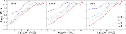
Host galaxy probability p(M*) as a function of stellar mass for the host galaxies of merging BNSs, BHNSs, and BBHs (from left to right) at z = 0.1 (red solid lines), 1 (green dotted lines), 2 (blue dashed lines), and 6 (purple dash–dotted lines).
These features are explained by the differences in the delay time distributions of the merging compact objects (see Mapelli et al. 2018, 2019). In fact, BNSs have a delay time distribution that approximately scales with ∼t−1 over the entire redshift range studied here, while merging BHNSs and BBHs tends to have a flatter delay time distribution at z ≤ 0.1.
The host probability associated with the smallest galaxies (M* ≲ 108 M⊙) is significantly higher at high redshift (z = 6). This is another effect of delay time, as only compact binaries with a very short delay time merge by z = 6, because the Universe at z ∼ 6 was younger than 1 Gyr and the first stars formed only few hundreds of Myr before. Hence, most of the compact binaries which merge at z ∼ 6 form and merge in the same galaxy.
The host probability as a function of mass increases almost monotonically from M* = 107 to ∼1010 M⊙, but then it shows a turnover at M* ≥ 1010 M⊙. The turnover point shifts towards higher masses as redshift decreases. Low-statistics effects affect our results at the high-mass tail: due to the size of the box of the eagle, ≤10 galaxies have stellar mass log (M*/M⊙) ≥ 11.69, 11.46, and 11.12 at z = 0.1, 1, and 2, respectively. The most evident effect of low-statistics is the oscillatory behaviour of the distribution for log (M*/M⊙) ≥ 11.7 at z = 0.1.
So far, our analysis directly took the distributions predicted by our model without taking into account detectability effects. However, we know that the current and future GW detectors introduce a bias in the observed distributions of compact mergers that should directly impact the evaluation of the host galaxy probability. To account for this, we have created catalogues of observed compact binary mergers by filtering our original catalogue using the framework already presented in previous works (Finn & Chernoff 1993; Dominik et al. 2015; Chen et al. 2018; Gerosa et al. 2018), and summarized in Appendix A. We highlight here that, given the computational cost of this analysis and the high number of binaries contained in the original catalogue (for instance, we have more than 6 × 10⁸ BNSs at z = 1), all the catalogues were downsampled in order to have a number of sources close to 107. This number represents |$\sim 1\!-\!20{{\ \rm per\ cent}}$| of the original intrinsic catalogues, and allows us to have manageable computation time. To check the validity of our downsampling procedure, we compared the values for p(M*) obtained with the full set and the downsampled one. We found a maximal percentage error value close to |$3 {{\ \rm per\ cent}}$|, indicating very little bias between the two sets.
Fig. 2 shows the values of p(M*) inferred from the downsampled catalogues that include detectability effects, considering advanced LIGO–Virgo design sensitivity and Einstein Telescope (hereafter ET) at z = 0.1, and 1. BNS and BHNS sources are not detected by advanced LIGO at z = 1 due to the lack of sensitivity of the instrument at this redshift value.
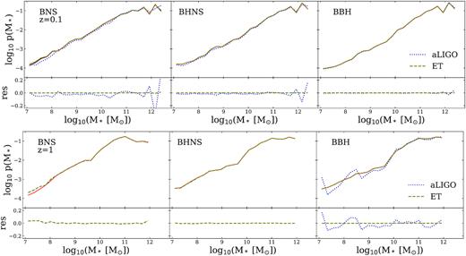
Host galaxy probability as a function of stellar mass, for the downsampled set without detectability effects (red solid line), and with detectability effects, considering advanced LIGO–Virgo design sensitivity (purple dotted line), and ET (green dashed line) at redshifts z = 0.1 (top) and z = 1 (bottom). The bottom panel of each cell shows the residuals between the host galaxy probability without detection effects and the one with detection effects for advanced LIGO–Virgo (purple dotted line) and ET (green dashed line).
At z = 0.1, including detectability effects does not change the general features of p(M*), that still favours galaxies with high mass. However, we do observe some bias introduced by detectability effects for advanced LIGO–Virgo, especially at high values of mass M* > 1011M⊙. We find values of residuals as high as 0.25 for BNSs, while the maximum value of the residuals peaks at 0.15 and 0.02 for BHNSs and BBHs, respectively (see Fig. 2). This trend is explained by the fact that BNSs at redshift z ∼ 0.1 are already close to the instrumental horizon of advanced LIGO–Virgo, resulting in a loss of |$~77{{\ \rm per\ cent}}$| of the sources after applying our filtering technique. For ET, we observe no differences between the two distributions and the residuals are almost always equal to zero. Once again, this is easily understood given that an ET-like detector can detect almost all compact binary mergers in our local Universe.
At z = 1, p(M*) does not change significantly when we consider the sensitivity of an ET-like observatory. The situation is very different for advanced LIGO–Virgo, since only BBHs can be detected at this redshift, with a loss of |$\sim 88{{\ \rm per\ cent}}$| of the intrinsic number of sources, resulting in a maximum value for the residual close to 0.2.
3.2 Host-galaxy probability: stellar mass and SFR
SFR is another key ingredient that needs to be considered in the analysis. Several studies have shown that there is an intrinsic correlation between the stellar mass and the SFR of galaxies (see e.g. Furlong et al. 2015; Sparre et al. 2015; Trayford et al. 2019). Figs 3–5 show the values of the host-galaxy probability as a function of stellar mass and SFR, p(M*, SFR), for merging BNSs, BHNSs, and BBHs, respectively, at z = 0.1, 1, 2, and 6. These figures also display the marginal probability p(SFR) depending on SFR only.
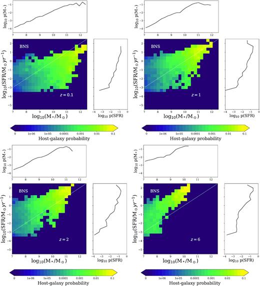
Host-galaxy probability as a function of M* and SFR for the hosts of BNS mergers at redshifts z = 0.1, 1, 2, and 6. The marginal histograms show the host galaxy probability as a function of SFR (p(SFR), right) and stellar mass (p(M*), top). The white dotted line represents a specific SFR = 10−10 yr−1.
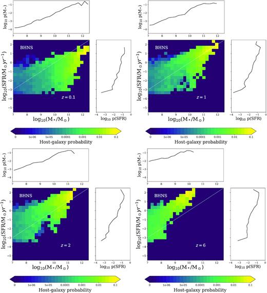
The same as Fig. 3, but for the host galaxies of BHNSs.
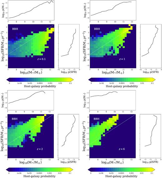
The same as Fig. 3, but for the host galaxies of BBHs.
Galaxies with higher values of SFR have a higher probability p(SFR) to host a merger, regardless of the compact object type. If we now take a look at the probability p(M*, SFR) as a function of both stellar mass and SFR, we see that galaxies with high values of both stellar mass and SFR have a higher probability of hosting a merger, for all type of compact objects and for all considered redshifts. The shape of the distributions also suggests that stellar mass is the main parameter influencing the host galaxy probability. In fact, for a fixed value of SFR, we observe more variation of the distribution than in the case where stellar mass is fixed. Quantitatively, we found that the ratio between the maximum and minimum (non-zero) value of the host galaxy probability is 10–100 higher when SFR is fixed, compared to the case where M* is fixed. Hence, according to our model, the stellar mass of the host galaxies of compact binary mergers is more important than SFR to characterize the host galaxy probability.
3.3 Host galaxy probability: Ks and B magnitudes
Galaxy surveys used for the EM follow-up of GW sources (such as GLADE and CLU, Dálya et al. 2018; Cook et al. 2019) do not include direct information on the stellar mass and SFR of galaxies. Rather, they contain B-band and Ks-band magnitudes as a proxy of SFR and stellar mass, respectively.
Hence, in order to facilitate the usage of our results in EM searches, we derive the host galaxy probability as a function of the rest-frame absolute magnitudes in B- and Ks-band, p(MB), and |$p(M_{\rm K_s})$|, respectively. To this purpose, we have extracted the rest-frame absolute magnitudes provided in the eagle data base. The magnitudes were computed for the galaxies with stellar mass above M* ∼ 1.81 × 10⁸ M⊙, and for the stellar emission including the effect of dust (see Trayford et al. 2019, for further details).
Fig. 6 shows the host galaxy probability as a function of the rest-frame absolute magnitudes in B and Ks band, p(MB), and |$p(M_{K_s})$|. The host galaxy probabilities are computed with the same methodology as explained in Sections 2.2 and 3.1, but replacing the stellar mass of each galaxy with its rest-frame magnitude. Both p(MB) and |$p(M_{K_s})$| grow as a function of MB and |$M_{K_s}$|, respectively.
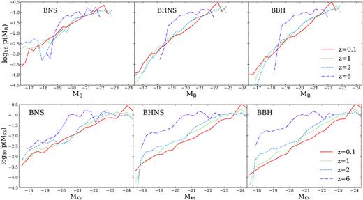
Host galaxy probability as a function of the rest-frame absolute magnitudes in B (top) and Ks band (bottom) for the host galaxies of merging BNSs, BHNSs, and BBHs (from left to right) at z = 0.1 (red solid lines), 1 (green dotted lines), 2 (blue dashed lines), and 6 (purple dash–dotted lines).
The peak of the host galaxy probability as a function of the Ks magnitude shifts to higher luminosities (i.e. more massive galaxies) as redshift decreases, following the same trend that we found for p(M*). This trend is stronger for the host galaxies of BHNSs and BBHs than for the host galaxies of BNSs.
In contrast, p(MB) does not show significant variations with redshift in the range z = 0.1–2. Indeed, the lack of a trend with redshift is similar to what we found for the host galaxy probability as a function of the SFR p(SFR). These results confirm that while the Ks magnitude is a good proxy for stellar mass, the B magnitude is affected by dust extinction, i.e. it is more a tracer of the SFR than a proxy for the stellar mass.
4 COMPARISON TO OTHER PRIORITIZATION STRATEGIES
Previous studies have developed prioritization strategies which include stellar mass (Ducoin et al. 2020) or B magnitude (Arcavi et al. 2017). Our method is complementary to such strategies for the following reasons:
Previous work assumes that the host-galaxy probability scales with the stellar mass (or with the B-band luminosity) based on heuristic arguments, such as the host-galaxy mass distribution of short gamma-ray bursts (Leibler & Berger 2010; Fong et al. 2013; Berger 2014), and on the results of previous theoretical studies (Mapelli et al. 2018; Toffano et al. 2019; Artale et al. 2020). Here, we directly compute a probability distribution from our astrophysical model. Hence, while our criterion is more model dependent than previous studies, it is also self-consistent and robustly motivated from an astrophysics point of view.
In previous work, the host galaxy probability is assumed to scale linearly with stellar mass (excluding possible corrections, such as the correction for galaxies without mass measurement introduced by Ducoin et al. 2020). In contrast, we do not need to assume a linear scaling. Rather, we assign specific weights to each stellar mass bin (and/or SFR bin), which are uniquely determined by our model. We show that there is a correlation between the merger rate per galaxy and the stellar mass, and this correlation is not simply a linear relation. Weighting this correlation is important to quantify deviations with respect to a linear scaling. Future detections of EM counterparts will help us to validate our criterion, giving us a feedback on our astrophysical model.
In our methodology, we can use not only the stellar mass but also the SFR: when not only the stellar mass is known but also the SFR, both data can be used to improve the prioritization.
We generalize our method to higher redshifts. This will become important for next generation ground-based GW detectors (Punturo et al. 2010; Kalogera et al. 2019; Reitze et al. 2019; Maggiore et al. 2020).
Ducoin et al. (2020) derive stellar masses from data using a specific calibration, while we follow a complementary approach: since observational catalogues usually do not contain stellar masses but magnitudes, we use the cosmological simulations to translate stellar masses and SFR into KS and B band, respectively. This can be done for other bands, making our criterion even more flexible. If the KS and/or the B magnitude, the stellar mass and/or the SFR are available for the galaxies in the error box, our tabulated probabilities can be used and convolved with sky localization as described in equation (4).
For example, we have convolved our ranking criterion with the stellar masses in the MANGROVE catalogue, to check consistency with the results of Ducoin et al. (2020). We found that, using their equation (4) to rank the possible host galaxies of GW170817, we obtain the same ranking for the first three galaxies of the catalogue, namely NGC 4993, IC 4197, and NGC 4970.
5 CONCLUSIONS
Understanding what are the properties of the most likely host galaxies of BNS, BHNS, and BBH mergers is fundamental for the EM follow-up of GW detections. Here, we discussed the host galaxy probability, i.e. the probability that a galaxy hosts a merging compact object as a function of its stellar mass and SFR at redshifts z = 0.1, 1, 2, and 6. Our methodology combines the results from the population synthesis code mobse (Giacobbo et al. 2018; Giacobbo & Mapelli 2018) together with galaxy catalogues from the cosmological simulation eagle (Schaye et al. 2015). With a Monte Carlo approach, we populate each galaxy in the eagle catalogue with BNSs, BHNSs, and BBHs.
Our results show that there is a strong dependence of the host galaxy probability on the stellar mass, p(M*), for all types of compact binaries: massive galaxies are more likely to host a compact-binary merger than low-mass galaxies. Moreover, the distribution shifts towards massive hosts as redshift decreases (see Fig. 1), as a consequence of the cosmic galaxy assembly and the delay time distribution of compact binary sources.
We also find that galaxies with higher SFR have a higher probability of hosting compact object mergers. Nevertheless, as shown in Figs 3, 4, and 5, the dependence on SFR is not as strong as the dependence on stellar mass. At a fixed stellar mass, p(M*, SFR) shows less significant variation compared to the case where SFR is fixed. Overall, the peak of the host probability at high SFR is mainly due to massive galaxies that in turn are forming more stars.
Our conclusions depend on the population-synthesis model and on the cosmological simulation. On the other hand, it is remarkable that both BNSs and BBHs show the same trend: their preferred host galaxies are the most massive ones and possibly the most star forming. This result indicates that the dependence on a specific population-synthesis model is not particularly strong, if we consider that the merger efficiency of BNSs marginally depends on metallicity in our models, while the merger efficiency of BBHs and BHNSs dramatically depends on progenitor’s metallicity. The key ingredient here is the delay time distribution, which is not strongly affected by model assumptions (Mapelli et al. 2019). Our results rely on the choice of the eagle simulation. In Artale et al. (2020), we have shown that our results are not significantly influenced by resolution, although we are not able to study galaxies with stellar mass M* < 107 and >1012 M⊙. The eagle appears to match some of the most important observables, such as the mass–metallicity relation of galaxies (De Rossi et al. 2017), the colour–magnitude diagram at z = 0 (Trayford et al. 2015), the evolution of the galaxy stellar mass function, and the cosmic SFR density evolution (Furlong et al. 2015; Trayford et al. 2019).
In the context of the EM follow-up of GW sources, our results can be implemented in ranking procedures applied for GW mergers detected by advanced LIGO–Virgo (Singer et al. 2016). The standard strategy consists in targeting galaxies within the skymap provided by the LVC using a complete galaxy catalogue such as GLADE (Dálya et al. 2018). Then, the galaxies are ranked adopting a criterion generally based on the 2D localization region, distance, and B-band magnitude (see e.g. Arcavi et al. 2017; Coughlin et al. 2018; Rana & Mooley 2019). Recently, Ducoin et al. (2020) proposed to use the stellar mass instead of the B-band magnitude in the ranking procedure.
Here, we propose a new astrophysically motivated criterion to compute the relative probability that a galaxy inside the LVC uncertainty box hosts a GW detection. If we calculate this host galaxy probability as a function of stellar mass only (p(M*)), our results are in agreement with the analytic model from Ducoin et al. (2020), and we find that high-mass galaxies are much more likely to host mergers than low-mass galaxies.
In addition, we also investigate what is the impact of including the SFR in our ranking criterion, which to our knowledge was never done before. While we find that the effect of SFR is less important than stellar mass, we observe that the probability that a galaxy hosts a merger is higher for high values of both stellar mass and SFR.
Galaxy catalogues usually do not include direct information on stellar mass and SFR. Hence, to facilitate the usage of our ranking criterion, we calculate the host galaxy probabilities p(Ks) and p(B) as a function of the Ks-band and B-band magnitudes. The former shows a similar trend to p(M*), while the latter is reminiscent of p(SFR), suggesting that Ks and B magnitudes are tracers of stellar mass and SFR, respectively.
Our host-galaxy probabilities can be implemented in future low-latency searches, providing a useful criterion to rank possible host galaxies within the sky localization map. The tables of the host-galaxy probabilities can be obtained online in table format.3
SUPPORTING INFORMATION
SupplementaryMaterial.zip
Please note: Oxford University Press is not responsible for the content or functionality of any supporting materials supplied by the authors. Any queries (other than missing material) should be directed to the corresponding author for the article.
ACKNOWLEDGEMENTS
We thank Walter Del Pozzo, Marica Branchesi, Stefan Grimm, Jan Harms, and Dario Rodriguez for their useful comments. MCA and MM acknowledge financial support from the Austrian National Science Foundation through FWF stand-alone grant P31154-N27 ‘Unraveling merging neutron stars and black hole – neutron star binaries with population synthesis simulations’. YB, NG, MM and FS acknowledge financial support by the European Research Council for the ERC Consolidator grant DEMOBLACK, under contract no. 770017. MS acknowledges funding from the European Union’s Horizon 2020 research and innovation programme under the Marie-Skłodowska-Curie grant agreement No. 794393. MP acknowledges funding from the European Union’s Horizon 2020 research and innovation programme under the Marie Skłodowska-Curie grant agreement no. 664931. We acknowledge the Virgo Consortium for making their simulation data available. The eagle simulations were performed using the DiRAC-2 facility at Durham, managed by the ICC, and the PRACE facility Curie based in France at TGCC, CEA, Bruyères-le-Châtel.
Footnotes
We refer to delay time as the time elapsed between the formation of the stellar progenitor to the merger of the binary compact object system.
See Appendix B, or alternatively https://github.com/mcartale/HostGalaxyProbability.
REFERENCES
APPENDIX A: JOINT PROBABILITY DISTRIBUTION ACCORDING TO THE DETECTABILITY OF GROUND-BASED INTERFEROMETERS
To produce catalogues of sources as observed by either LIGO–Virgo or ET, we follow a similar approach as done in previous works (see e.g. Finn & Chernoff 1993; Dominik et al. 2015; Gerosa et al. 2018). Here, we briefly summarize the main details of this approach.
In practice, we evaluate the optimal SNR ρopt for each source in our catalogue and then compute the detection probability as in equation (A2). We then draw a random number |$\epsilon \sim \mathcal {U}[0,1]$| and add the source with probability pdet in our catalogues of detectable sources that are used to produce Fig. 2.
APPENDIX B: SUPPLEMENTARY MATERIAL: HOST-GALAXY PROBABILITY TABLES
The host-galaxy probabilities for BNSs, BHNSs, and BBHs at z = 0.1, 1, 2, and 6 presented in Figs 3–5 can be obtained in table format in the supplementary material online. Alternatively, the tables are also available on https://github.com/mcartale/HostGalaxyProbability. Our results can be directly implemented in low-latency searches of EM counterparts as described in Section 2.
Table of the host galaxy probability as a function of M* and SFR, for BNSs at z = 0.1, corresponding to the results presented in Fig. 5. Stellar masses are in units of M⊙, while SFR is in yr−1 M⊙. Note: This table is presented in its entire version in https://github.com/mcartale/HostGalaxyProbability. An abbreviated version is shown here for guidance.
| log (M*min) | log (M*max) | log (SFRmin) | log (SFRmax) | p(M*, SFR) |
|---|---|---|---|---|
| 7.0 | 7.229 | −5.5 | −5.167 | 0.0 |
| 7.0 | 7.229 | −5.167 | −4.833 | 0.0 |
| 7.0 | 7.229 | −4.833 | −4.5 | 0.0 |
| 7.0 | 7.229 | −4.5 | −4.167 | 0.0 |
| 7.0 | 7.229 | −4.167 | −3.833 | 0.0 |
| 7.0 | 7.229 | −3.833 | −3.5 | 0.0 |
| 7.0 | 7.229 | −3.5 | −3.167 | 1.830809731518871e−06 |
| 7.0 | 7.229 | −3.167 | −2.833 | 3.876326253400243e−06 |
| 7.0 | 7.229 | −2.833 | −2.5 | 6.905726150471546e−06 |
| 7.0 | 7.229 | −2.5 | −2.167 | 6.131134402365386e−06 |
| 7.0 | 7.229 | −2.167 | −1.833 | 1.555843012065854e−05 |
| 7.0 | 7.229 | −1.833 | −1.5 | 1.423655645772669e−05 |
| 7.0 | 7.229 | −1.5 | −1.167 | 3.249632877051857e−05 |
| 7.0 | 7.229 | −1.167 | −0.833 | 2.3823821312203474e−05 |
| 7.0 | 7.229 | −0.833 | −0.5 | 2.2302151013959734e−05 |
| 7.0 | 7.229 | −0.5 | −0.167 | 8.486969225985846e−06 |
| 7.0 | 7.229 | −0.167 | 0.167 | 0.0 |
| 7.0 | 7.229 | 0.167 | 0.5 | 3.829732624985512e−07 |
| 7.0 | 7.229 | 0.5 | 0.833 | 0.0 |
| 7.0 | 7.229 | 0.833 | 1.167 | 0.0 |
| 7.0 | 7.229 | 1.167 | 1.5 | 0.0 |
| 7.0 | 7.229 | 1.5 | 1.833 | 0.0 |
| 7.0 | 7.229 | 1.833 | 2.167 | 0.0 |
| 7.0 | 7.229 | 2.167 | 2.5 | 0.0 |
