


ABSTRACT
We present an overview and description of the e-MERGE Survey (e-MERLIN Galaxy Evolution Survey) Data Release 1 (DR1), a large program of high-resolution 1.5-GHz radio observations of the GOODS-N field comprising ∼140 h of observations with enhanced-Multi-Element Remotely Linked Interferometer Network (e-MERLIN) and ∼40 h with the Very Large Array (VLA). We combine the long baselines of e-MERLIN (providing high angular resolution) with the relatively closely packed antennas of the VLA (providing excellent surface brightness sensitivity) to produce a deep 1.5-GHz radio survey with the sensitivity (|${\sim}1.5\, \mu$| Jy beam−1), angular resolution (0.2–0.7 arcsec) and field-of-view (∼15 × 15 arcmin2) to detect and spatially resolve star-forming galaxies and active galactic nucleus (AGN) at |$z$| ≳ 1. The goal of e-MERGE is to provide new constraints on the deep, sub-arcsecond radio sky which will be surveyed by SKA1-mid. In this initial publication, we discuss our data analysis techniques, including steps taken to model in-beam source variability over an ∼20-yr baseline and the development of new point spread function/primary beam models to seamlessly merge e-MERLIN and VLA data in the uv plane. We present early science results, including measurements of the luminosities and/or linear sizes of ∼500 galaxies selected at 1.5 GHz. In combination with deep Hubble Space Telescope observations, we measure a mean radio-to-optical size ratio of re-MERGE/rHST ∼ 1.02 ± 0.03, suggesting that in most high-redshift galaxies, the ∼GHz continuum emission traces the stellar light seen in optical imaging. This is the first in a series of papers that will explore the ∼kpc-scale radio properties of star-forming galaxies and AGN in the GOODS-N field observed by e-MERGE DR1.
1 INTRODUCTION
Historically, optical and near-infrared (NIR) surveys have played a leading role in measuring the integrated star formation history of the Universe (e.g. Lilly et al. 1996; Madau et al. 1996), however, in recent years a panchromatic (i.e. X-ray–radio) approach has become key to achieving a consensus view on galaxy evolution (e.g. Scoville et al. 2007; Driver et al. 2009). Since the pioneering work in the FIR and sub-millimetre wavebands undertaken with the Submillimeter Common-User Bolometer Array (SCUBA) on the James Clerk Maxwell Telescope, it has been established that a significant fraction of the integrated cosmic star formation (up to |${\sim}50{{\ \rm per\ cent}}$| at |$z$| ∼ 1–3; Swinbank et al. 2014; Barger et al. 2017) has taken place in heavily dust-obscured environments, which can be difficult (or impossible) to measure fully with even the deepest optical/near-IR data (e.g. Barger et al. 1998; Seymour et al. 2008; Hodge et al. 2013; Casey, Narayanan & Cooray 2014). Within this context, deep interferometric radio continuum observations are an invaluable complement to studies in other wavebands, providing a dust-unbiased tracer of star formation (e.g. Condon 1992; Smolčić et al. 2009), allowing us to track the build-up of stellar populations through cosmic time without the need to rely on uncertain extinction corrections. Moreover, radio continuum observations also provide a direct probe of the synchrotron emission produced by active galactic nuclei (AGNs), which are believed to play a crucial role in the evolution of their host galaxies via feedback effects (Best et al. 2006; Schaye et al. 2015; Harrison et al. 2018).
The radio spectra of galaxies at ≳1 GHz frequencies are typically thought to result from the sum of two power-law components (e.g. Condon 1992; Murphy et al. 2011). At frequencies between νrest ∼ 1–10 GHz, radio observations trace steep-spectrum (α ∼ −0.8, where Sν ∝ να) synchrotron emission, which can be produced either by supernova explosions (in which case it serves as a dust-unbiased indicator of the star formation rate, SFR, over the past ∼10–100 Myr: Bressan, Silva & Granato 2002) or from accretion processes associated with the supermassive black holes at the centres of AGN hosts. At higher frequencies (νrest ≳ 10 GHz), radio observations trace flatter-spectrum (α ∼ −0.1) thermal free–free emission, which signposts the scattering of free-electrons in ionized H ii regions around young, massive stars, and thus is considered to be an excellent tracer of the instantaneous SFR.
This dual origin for the radio emission in galaxies (i.e. star formation and AGN activity) makes the interpretation of monochromatic radio observations of unresolved, distant galaxies non-trivial. To determine the origin of radio emission in distant galaxies requires (a) the angular resolution and surface brightness sensitivity to morphologically decompose (extended) star formation and radio jets from (point-like) nuclear activity (e.g. Baldi et al. 2018; Jarvis et al. 2019), and/or (b) multifrequency observations that provide the spectral index information necessary to measure reliable rest-frame radio luminosities. These allow galaxies that deviate from the FIR/radio correlation (FIRRC) to be identified, a correlation on which star-forming galaxies at low and high redshift are found to lie (e.g. Helou, Soifer & Rowan-Robinson 1985; Bell 2003; Ivison et al. 2010; Thomson et al. 2014; Magnelli et al. 2015).
The magnification afforded by gravitational lensing provides one route towards probing the obscured star formation and AGN activity via radio emission in individual galaxies at high redshift (e.g. Hodge et al. 2015; Thomson et al. 2015), however, in order to produce a statistically robust picture of the interplay between these processes for the high-redshift galaxy population, in general, and to obtain unequivocal radio counterparts for close merging systems requires sensitive (|$\sigma _{\rm rms}\sim 1\, \mu$|Jy beam−1) radio imaging over representative areas (≳10 × 10 arcmin2) with ∼kpc (i.e. sub-arcsecond) resolution. The Karl G. Jansky Very Large Array (VLA) is currently capable of delivering this combination of observing goals in S-band (3 GHz), X-band (10 GHz), and at higher frequencies. However, by |$z$| ∼ 2 these observations probe rest-frame frequencies νrest ≳ 10–30 GHz, a region of the radio spectrum in which the effects of spectral curvature may become important due to the increasing thermal free–free component at high-frequencies (e.g. Murphy et al. 2011), and/or spectral steepening due to cosmic-ray effects (Galvin et al. 2018; Thomson et al. 2019) and free–free absorption (Tisanić et al. 2019). This potential for spectral curvature complicates efforts to measure the rest-frame radio luminosities (conventionally, |$L_{\rm 1.4\, GHz}$|) of high-redshift galaxies from these higher-frequency observations.
Furthermore, the instantaneous field of view (FoV) of an interferometer is limited by the primary beam, θPB, which scales as λ/D, with D being the representative antenna diameter. At 1.4 GHz the FoV of the VLA’s 25-m antennas is θPB ∼ 32 arcmin, while the angular resolution offered by its relatively compact baselines (Bmax = 36.4 km) is θres ∼ 1.5 arcsec. This corresponds to ∼12 kpc at ∼ 2, and is therefore insufficient to morphologically study the bulk of the high-redshift galaxy population, which have optical sizes of only a few kpc (van der Wel et al. 2014). At 10 GHz, in contrast, the angular resolution of the VLA is θres ∼ 0.2 arcsec (∼1.5 kpc at = 2), but the FoV shrinks to θPB ∼ 4.5 arcmin. This large (a factor ∼50 ×) reduction in the primary beam area greatly increases the cost of surveying deep fields over enough area to overcome cosmic variance (e.g Murphy et al. 2017), particularly given that the positive k-correction in the radio bands means that these observations probe an intrinsically fainter region of the rest-frame radio SEDs of high-redshift galaxies to begin with.
Over the coming decade the SKA1-mid and its precursor instruments (including MeerKAT and ASKAP) will add new capabilities to allow the investigation of the faint extragalactic radio sky (Prandoni & Seymour 2015; Jarvis et al. 2016; Taylor & Jarvis 2017). At ∼1-GHz observing frequencies these extremely sensitive instruments will reach (confusion limited) |${\sim}\, \mu$|Jy beam−1 sensitivities over tens of square degrees in area, but with an angular resolution of ≳10 arcsec, corresponding to a linear resolution of ≳80 kpc at |$z$| = 1. Crucially, this means that a significant fraction of the high-redshift star-forming galaxies and AGN detected in these surveys will remain unresolved (see Fig. 1).
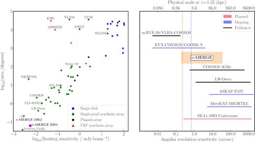
Left-hand panel: sky area versus sensitivity (detection limit or 5σrms) for selected radio surveys, highlighting the sensitivity of e-MERGE Data Release 1 (DR1) with respect to existing studies in the ∼GHz window. In a forthcoming DR2, including approximately four times more e-MERLIN uv data, we will quadruple the area and double the sensitivity of e-MERGE offering the first sub-|$\, \mu$|Jy beam−1 view of the deep 1.5-GHz radio sky. Right-hand panel: a comparison of the angular scales probed by selected ∼GHz-frequency radio continuum surveys; the right-most edge of each line represents the Largest Angular Scale (θLAS) probed by the corresponding survey, and is defined by the shortest antenna spacing in the relevant telescope array. The left-most edge is the angular resolution (θres) defined by the naturally weighted point spread function (PSF) of each survey. Vertical lines at 0.25 and 0.70 arcsec (corresponding to ∼2 and ∼7 kpc at |$z$| = 1.25, respectively) represent the typical effective radii of massive (M⋆ ∼ 1011 M⊙) early- and late-type galaxies seen in optical studies (van der Wel et al. 2014). While the area coverage of e-MERGE DR1 is modest compared with other surveys, its combination of high sensitivity and sub-arcsecond angular resolution offers a unique view of the population of radio-selected SFGs and AGN at high redshift. The long baselines of e-MERLIN bridge the gap between VLA and very long baseline interferometry (VLBI) surveys, offering sensitive imaging at ∼kpc scale resolution in the high-redshift Universe. e-MERGE thus provides a crucial benchmark for the sizes and morphologies of the high redshift radio source population, and delivers a glimpse of the radio sky that will be studied by SKA1-mid in the next decade.
There is thus a need for high angular resolution and high sensitivity, wide-field radio observations in the ∼GHz radio window to complement surveys which are underway in different frequency bands, and with different facilities. To address this, we have been conducting a multitiered survey of the extragalactic sky using the enhanced-Multi-Element Remotely Linked Interferometer Network (e-MERLIN), the UK’s national facility for high angular resolution radio astronomy (Garrington et al., in preparation), along with observations taken with the VLA. This ongoing project – the e-MERLIN Galaxy Evolution Survey (e-MERGE) – exploits the unique combination of the high angular resolution and a large collecting area of e-MERLIN, and the excellent surface brightness sensitivity of the VLA. The combination of these two radio telescopes allows the production of radio maps, which exceed the specifications of either instrument individually, and thus allows synchrotron emission due to both star formation activity and AGN to be mapped in the high-redshift Universe.
1.1 e-MERGE: an e-MERLIN legacy project
e-MERLIN is an array of seven radio telescopes spread across the UK (having a maximum baseline length Bmax = 217 km), with antenna stations connected via optical fibre links to the correlator at Jodrell Bank Observatory. e-MERLIN is an inhomogeneous array comprised the 76-m Lovell Telescope at Jodrell Bank (which provides |${\sim}58{{\ \rm per\ cent}}$| of the total e-MERLIN collecting area), one 32-m antenna near Cambridge (which provides the longest baselines) and five 25-m antennas, three of which are identical in design to those used by the VLA.
Due to the inhomogeneity of the e-MERLIN telescopes, the primary beam response (which defines the sensitivity of the array to emission as a function of radial distance from the pointing centre) is complicated (see Section 2.5.2), however, to first order it can be parametrized at 1.5 GHz as a sensitive central region ∼15 arcmin in diameter (arising from baselines which include the Lovell Telescope) surrounded by an ∼45 arcmin annulus, which is a factor of ∼2 times less sensitive, and arises from baselines between pairs of smaller telescopes.
Our target field for e-MERGE is the Great Observatories Origins Deep Survey North field (GOODS-N, |$\alpha =12^{\rm h}36^{\rm m}49{{.\!\!\!^{{\rm {\small {s}}}}}}40$|, δ = +62○12′58|${^{\prime\prime}_{.}}$|0; Dickinson et al. 2003), which contains the original Hubble Deep Field (Williams et al. 1996). Due to the extent of the deep multiwavelength coverage, GOODS-N remains one of the premier deep extra-galactic survey fields. The field was first observed at ∼1.4-GHz (L-band) radio frequencies by the VLA by Richards (2000), yielding constraints on the ∼10–|$100\, \mu$|Jy radio source counts. Using a sample of 371 sources, Richards (2000) found flattening of the source counts (normalized to N(S) ∝ S3/2) below |$S_{\rm 1.4\, GHz}=100\, \mu$|Jy. Later, Morrison et al. (2010), using the original Richards (2000) observations plus a further 121 h of (preupgrade) VLA observations achieved improved constraints on the radio source counts, finding them to be nearly Euclidian at flux densities |${\lesssim}100\, \mu$|Jy and with a median source diameter of ∼1.2 arcsec, i.e. close to the angular resolution limit of the VLA. Muxlow et al. (2005) subsequently published 140 h of 1.4-GHz observations of GOODS-N with MERLIN, obtaining high angular resolution postage stamp images of 92 of the Richards (2000) VLA sources, a slight majority of which (55/92) were found to be associated with Chandra X-ray sources (Brandt et al. 2001; Richards et al. 2007), and hence were classified as possible AGN. The angular size distribution of these bright radio sources peaks around a largest angular scale of θLAS ∼ 1.0 arcsec, but with the tail of more extended sources out to θLAS ∼ 4.0 arcsec.
More recently, the field has been re-observed with the upgraded VLA by Owen (2018), who extracted a catalogue of 795 radio sources over the inner ∼9 arcmin of the field. Owen (2018) measured a linear size distribution in the radio, which peaks at ∼10 kpc, finding the radio emission in most galaxies to be larger than the galaxy nucleus but smaller than the galaxy optical isophotal size (∼15–20 kpc).
In this paper, we present a description of our updated e-MERLIN observations of the field, which along with an independent reduction of the Owen (2018) VLA observations and older VLA/MERLIN observations, constitute e-MERGE DR1. This data release will include approximately one-fourth of the total e-MERLIN L-Band (1–2 GHz) observations granted to the project (i.e. 140 of 560 h), which use the same pointing centre as all the previous deep studies of the field discussed in the preceding paragraphs. We use VLA observations to fill the inner portion of the uv plane, which is not well sampled by e-MERLIN, in order to enhance our sensitivity to emission on ≳1 arcsec scales. We compare the survey area, sensitivity and angular resolution of e-MERGE with those of other state-of-the-art deep, extragalactic radio surveys in Fig. 1. In addition to our L-band observations, e-MERGE DR1 includes the seven-pointing VLA C-Band (5.5-GHz) mosaic image previously published by Guidetti et al. (2017). We summarize our e-MERGE DR1 observations in Table 1, list the central coordinates of each e-MERGE pointing (1.5 and 5.5 GHz using both telescopes) in Table 2, and show the e-MERGE survey footprint (including both existing and planned future observations) in Fig. 2.
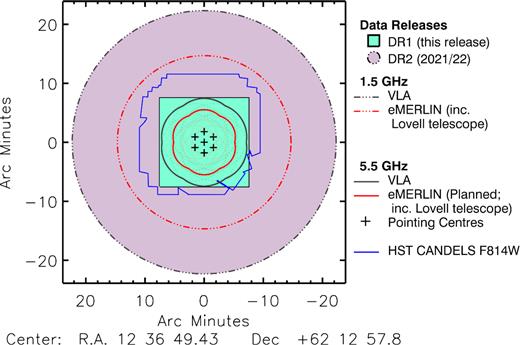
The e-MERGE survey layout, showing the current (DR1; black box) and planned future (DR2; lilac circle) survey areas. e-MERGE 1.5-GHz observations comprise a single deep pointing which includes 40 h of VLA and 140 h of e-MERLIN observations, encompassing the Hubble Space Telescope (HST) Cosmic Assembly Near-infrared Deep Extragalactic Legacy Survey (CANDELS) field (shown in blue). Our DR1 area is limited by time and bandwidth smearing effects (both of which increase as a function of radial distance from the phase centre: see Section 2.5.3 for details). In a forthcoming DR2, we will include an additional ∼400 h of observed e-MERLIN 1.5-GHz data, which will be processed without averaging in order to allow the full primary beam of the 25 m e-MERLIN and VLA antennas to be mapped. e-MERGE DR1 includes the 14-h seven-pointing 5.5-GHz VLA mosaic image published by Guidetti et al. (2017), which will be supplemented in our forthcoming DR2 with an additional 42 h of VLA and ∼380 h of e-MERLIN 5.5-GHz observations which share the same pointing centres. Our planned 5.5-GHz mosaic will eventually reach an angular resolution of ∼50 mas at |$\sigma _{\rm 5.5\, GHz}\sim 0.5\, \mu$|Jy beam−1. Note that the VLA 5.5-GHz pointings are significantly oversampled with respect to the VLA primary beam in order to facilitate uv plane combination with data from e-MERLIN, whose primary beam is significantly smaller than the VLA’s when the 76-m Lovell telescope is included in the array.
Summary of observations included within e-MERGE DR1.
| Telescope | Reference | Array | Project | Total time | Epoch(s) | Typical sensitivity |
|---|---|---|---|---|---|---|
| frequency | configuration | code | (h) | (μJy beam−1) | ||
| e-MERLIN a | 1.5 GHz | – | LE1015 | 140 | 2013 Mar and Apr, 2013 Dec, 2015 Jul | 2.81 |
| VLAb | 1.5 GHz | A | TLOW0001 | 38 | 2011 Aug and Sep | 2.01 |
| MERLINc | 1.4 GHz | – | – | 140 | 1996 Feb–1997 Sep | 5.70 |
| VLAc, d | 1.4 GHz | A | – | 42 | 1997 Sep–2000 May | 7.31 |
| VLAe, f | 5.5 GHz | B | 13B-152 | 2.5 | 2013 Sep | 7.90 |
| VLAe, f | 5.5 GHz | A | 12B-181 | 14 | 2012 Oct | 3.22 |
Pointing centres for the e-MERGE observations. The same positions are (or will be) used for both VLA and e-MERLIN observations at a given frequency.
| Band | RA | Dec. |
|---|---|---|
| [hms (J2000)] | [dms (J2000)] | |
| L (1.5 GHz) | |$12^{\rm h}36^{\rm m}49{{.\!\!\!^{{\rm {\small {s}}}}}}40$| | +62○12′58|${^{\prime\prime}_{.}}$|0 |
| C (5.5 GHz) | |$12^{\rm h}36^{\rm m}49{{.\!\!\!^{{\rm {\small {s}}}}}}40$| | +62○12′58|${^{\prime\prime}_{.}}$|0 |
| |$12^{\rm h}36^{\rm m}49 {.\!\!\!\!^{{\rm {\small {s}}}}}40$| | +62○14′46|${^{\prime\prime}_{.}}$|0 | |
| |$12^{\rm h}36^{\rm m}36{{.\!\!\!^{{\rm {\small {s}}}}}}00$| | +62○13′52|${^{\prime\prime}_{.}}$|0 | |
| |$12^{\rm h}36^{\rm m}36{{.\!\!\!^{{\rm {\small {s}}}}}}00$| | +62○12′02|${^{\prime\prime}_{.}}$|0 | |
| |$12^{\rm h}36^{\rm m}49{{.\!\!\!^{{\rm {\small {s}}}}}}40$| | +62○11′10|${^{\prime\prime}_{.}}$|0 | |
| |$12^{\rm h}37^{\rm m}02{{.\!\!\!^{{\rm {\small {s}}}}}}78$| | +62○12′02|${^{\prime\prime}_{.}}$|0 | |
| |$12^{\rm h}37^{\rm m}02{{.\!\!\!^{{\rm {\small {s}}}}}}78$| | +62○13′52|${^{\prime\prime}_{.}}$|0 |
We describe the design, execution, and data reduction strategies of e-MERGE DR1 in detail in Section 2, including a discussion of the wide-field imaging techniques, which we have developed to combine and image our e-MERLIN and VLA observations in Section 2.5. We present early science results from e-MERGE DR1 in Section 3, including the luminosity–redshift plane and angular size distribution of ∼500 high-redshift SFGs/AGN (∼250 of which benefit from high-quality photometric redshift information from the literature), and demonstrate the image quality via a brief study of a representative |$z$| = 1.2 submillimetre-selected galaxy (SMG) selected from our wide-field (θPB = 15 arcmin), sensitive (|${\sim}2\, \mu$|Jy beam−1), high-resolution (θres ∼ 0.5 arcsec) 1.5-GHz imaging of the GOODS-N field.1 Finally, we summarize our progress so far and outline our plans for future science delivery from e-MERGE (including the delivery of the full DR1 source catalogue) in Section 4. Throughout this paper, we use a Planck 2018 Cosmology with H0 = 67.4 km s−1 Mpc−1 and Ωm = 0.315 (Planck Collaboration VI 2018).
2 OBSERVATIONS AND DATA REDUCTION
2.1 e-MERLIN 1.5 GHz
The cornerstone of e-MERGE DR1 is our high-sensitivity, high-resolution L-band (1.25–1.75 GHz; central frequency of 1.5 GHz) imaging of the GOODS-N field, which we observed with e-MERLIN in five epochs between 2013 March–2015 July (a total on-source time of 140 h). In the standard observing mode, these e-MERLIN observations yielded time resolution of 1 s/integration and frequency resolution of 0.125 MHz/channel. The e-MERLIN frequency coverage is comprised eight spectral windows (spws) with 512 channels per spw per polarization. We calibrated the flux density scale using ∼30-min scans of 3C 286 at the beginning of each run, and tracked the complex antenna gains using regular ∼5-min scans of the bright phase reference source J1241+6020, which we interleaved between 10-min scans on the target field. We solved for the bandpass response of each observation using an ∼30-min scan of the standard e-MERLIN L-band bandpass calibration source, OQ 208 (1407+284). After importing the raw telescope data in to the NRAO Astronomical Image Processing System (|$\cal AIPS$|: Greisen 2003), we performed initial a priori flagging of known bad data – including scans affected by hardware issues and channel ranges known to suffer from persistent severe radio frequency interference (RFI) – using the automated serpent tool (Peck & Fenech 2013), before averaging the data by a factor of 4 times in frequency (to 0.5-MHz resolution) in order to reduce the data volume, using the |$\cal AIPS$| task splat. The discretization of interferometer uv data in time and frequency results in imprecisions in the (u, |$v$|) coordinates assigned to visibilities, which inevitably induces ‘smearing’ effects in the image plane: the effect of this frequency averaging on the image fidelity will be discussed in Section 2.5.3.
Next, we performed a further round of automated flagging to excise bad data, before further extensive manual flagging of residual time-variable and low-level RFI was carried out.
2.1.1 Amplitude calibration and phase referencing
We set the flux density scale for our observations using a model of 3C 286 along with the flux density measured by Perley & Butler (2013).
The delays and phase corrections were determined using a solution interval matching the calibrator scan lengths. Any significant outliers were identified and removed. Initial phase calibration was performed for the flux calibrator using a model of the source, and for the phase and bandpass calibrators assuming point source models. These solutions were applied to all sources and initial bandpass corrections (not including the intrinsic spectral index of OQ 208) were derived. The complex gains (phase and amplitude) were iteratively refined, with solutions inspected for significant outliers after each iteration to identify and exclude residual low-level RFI before the complex gain calibration was repeated.
The solution table containing the complex gains was used to perform an initial bootstrapping of the flux density from 3C 286 to the phase and bandpass calibrator sources. Exploiting the large fractional bandwidth of e-MERLIN (Δν/ν ∼ 0.33), these bootstrapped flux density estimates were subsequently improved by fitting the observed flux densities for J1241+6020 and OQ 208 linearly across all eight spws.
With the flux density scale and the spectral indices of the phase and bandpass calibrators thus derived, the bandpass calibration was improved, incorporating the intrinsic source spectral index. The complex gains were improved and then applied to all sources, including the target field. Finally, the target field was split from the multisource data set and the data weights were optimized based on the post-calibration baseline rms noise.
2.1.2 Self-calibration
We identified the brightest 26 sources (|$S_{\rm 1.5\, GHz}\ge 120\, \mu$|Jy) in the GOODS-N field at 1.5 GHz (guided by the catalogue of Muxlow et al. 2005) and produced e-MERLIN thumbnail images over a 5 × 5 arcsec2 region centred on each source. The sky model generated from these thumbnail images was used to produce a multisource model for phase-only self-calibration. This used a solution interval equal to the scan duration and was repeated until the phase solution converged to zero (typically within ∼3 iterations per epoch of data).
2.1.3 Variability, flux density, and astrometric cross-checks
Previous studies have shown that the fraction of sub-|$100\mu$|Jy variable radio sources is low (a few per cent, e.g. Mooley et al. 2016; Radcliffe et al. 2019). However, relatively small levels of intrinsic flux density variability of sources in the field, along with any small discrepancies in the relative flux density scale assigned to each epoch, will result in errors in the final combined image if not properly accounted for.
In order to assess and mitigate the effect of intrinsic source variability in our final, multi-epoch data set, each epoch of e-MERLIN and VLA data was imaged and catalogued separately using the flood-filling algorithm BLOBCAT (Hales et al. 2012), using rms maps generated by the accompanying BANE software (Hancock, Trott & Hurley-Walker 2018). We cross-checked the catalogues from each epoch to identify sources with significant intrinsic variability (|${\gtrsim}15{{\ \rm per\ cent}}$|; greater than the expected accuracy of the flux density scale), finding one such strongly variable source in the e-MERLIN observations and two in the VLA observations, and modelled and subtracted these from the individual epochs (see Section 2.4). The flux densities of the remaining (non-variable) sources were then compared to assess for epoch-to-epoch errors on the global flux density scale. We found the individual epochs to be broadly consistent, with the average integrated flux densities of non-variable sources differing by less than ∼10 per cent. Nevertheless, to correct these small variations, a gain table was generated and applied to bring each epoch to a common flux density scale (taken from the e-MERLIN epoch with the lowest rms noise, |$\sigma _{\rm 1.5\, GHz}$|).
In addition, the astrometry of each epoch was compared and aligned to the astrometric solutions derived by recent European VLBI Network (EVN) observations of the GOODS-N field (Radcliffe et al. 2018). By comparing the positions of 22 EVN-detected sources that are also in e-MERGE, we measured a systematic linear offset of ∼15 mas in RA (corresponding to |${\sim}5{{\ \rm per\ cent}}$| of the 0.3 arcsec e-MERLIN PSF and |${\sim}1{{\ \rm per\ cent}}$| of the 1.5 arcsec VLA PSF). This offset does not vary between epochs, and no correlation in the magnitude of the offset with the distance from the pointing centre was found, which indicates there are no significant stretch errors in the field. We determined that this offset arose due to an error in the recorded position of the phase reference source (Radcliffe et al. 2018), and corrected for this by applying a linear 15 mas shift to the e-MERLIN data sets. In this manner, we have astrometrically tied the e-MERGE DR1 uv data and images to the International Celestial Reference Frame to an accuracy of ≤10 mas.
2.2 VLA 1.5 GHz
To both improve the point source sensitivity of our e-MERGE data set and provide crucial short baselines needed to study emission on ≳1arcsec scales, 38 h (8 epochs of 4–6 h) of VLA L-band data were obtained in 2011 August–September using the A-array configuration between |$1\mbox{-}2\, {\rm GHz}$| (VLA project code TLOW0001). These data have been previously published by Owen (2018), and use a 1 s integration time and 1-MHz/channel frequency resolution, with 16 spws of 64 channels each, providing a total bandwidth of 1.024 GHz. We retrieved the raw, unaveraged data from the archive and processed them using a combination of the VLA casa pipeline (McMullin et al. 2007), along with additional manual processing steps. Initial flagging was performed using aoflagger (Offringa, van de Gronde & Roerdink 2012), before further automated flagging and initial calibration was applied using the VLA scripted pipeline packaged with casa version 4.3.1. Flux density bootstrapping was performed using 3C 286, while bandpass corrections were derived using the bright calibrator source 1313+6735 (which was also used for the delay and phase tracking). After pipeline calibration, the optimal data weights were derived based upon the rms scatter of the calibrated data set. Finally, one round of phase-only self-calibration on each epoch of data was performed using a sky model of the central 5-arcmin area (for which any resultant calibration errors due to the primary beam attenuation are expected to be minimal), and the data were exported with 3s time averaging.
The uv coverage attained by combining these VLA observations with the e-MERLIN observations discussed in the previous section is shown in Fig. 3.
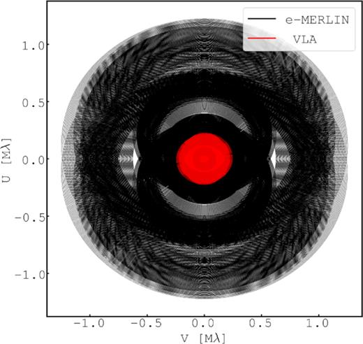
uv coverage of the combined e-MERLIN plus VLA 1.5-GHz data set presented in Section 2. The long (Bmax ∼ 217 km) baselines of e-MERLIN hugely extend the VLA-only uv coverage, while the presence of short baselines from the VLA (B ∼ 0.68–36.4 km) overlap and fill the inner gaps in e-MERLIN’s uv coverage due to its shortest usable baseline length of Bmin ∼ 10 km. The combined resolving power of both arrays provides seamless imaging capabilities with sensitivity to emission over ∼0.2–40 arcsec spatial scales.
2.3 Previous 1.4-GHz VLA + MERLIN observations
To maximize the sensitivity of the e-MERGE DR1 imaging products, we make use of earlier MERLIN and VLA uv data sets obtained between 1996–2000, i.e. prior to the major upgrades carried out to both instruments in the last decade. A total of 140 h of MERLIN and 42 h of preupgrade VLA (A-configuration) 1.5-GHz data share the same phase centres as our more recent e-MERLIN and post-upgrade VLA observations. Full details of the data reduction strategies employed for these data sets are presented in Muxlow et al. (2005) and Richards (2000), respectively. These data sets have a much-reduced frequency coverage compared to the equivalent post-2010 data sets, i.e. the MERLIN observations have 0.5 MHz/channel over 31 channels (yielding 15 MHz total bandwidth) while the legacy VLA observations have 3.125 MHz/channel over 14 channels (i.e. 44 MHz total bandwidth).
These single-polarization legacy VLA and MERLIN data sets were not originally designed to be combined in the uv plane, due to differences in channel arrangements of the VLA and MERLIN correlators. However, modern data-processing techniques nevertheless allow this uv plane combination to be achieved. We gridded both data sets on to a single channel (at a central reference frequency of 1.42 GHz) by transforming the u, |$v$|, and |$w$| coordinates from the multifrequency synthesis gridded coordinates. This gridding ensures that the full uv coverage is maintained during the conversion, with appropriate weights calculated in proportion to the sensitivity of each baseline within each array, and was performed within |$\cal AIPS$| by use of the split and dbcon tasks in a hierarchical manner. From these pseudo-single channels, single-polarization data sets, the data were then transformed into a Stokes I casa Measurement Set format via the following steps: (i) A duplicate of each data set was generated, with the designated polarization converted from RR to LL; (ii) the |$\cal AIPS$| task vbglu was used to combine the two polarizations into one data set with two spws; (iii) the |$\cal AIPS$| task fxpol was used to re-assign the spws into a data set containing one spw with a single channel per polarization. Finally, these data sets were then exported from |$\cal AIPS$| as uvfits files and converted to Measurement Set format using the casa task importuvfits, to facilitate eventual uv plane combination with the new e-MERLIN and VLA e-MERGE observations. We discuss the details of how our L-band data from both (e)MERLIN and old/new VLA were combined in the uv plane and imaged jointly in Section 2.5.
2.4 Subtraction of bright sources from 1.5-GHz e-MERLIN and VLA data
The combination of extremely bright sources located away from the phase centre of an interferometer and small gain errors in the data (typically caused by primary beam attenuation and atmospheric variations across the field) can produce unstable sidelobe structure within the target field which cannot be deconvolved from the map, limiting the dynamic range of the final clean map. These effects can be mitigated (while imaging) using direction-dependent calibration methods, such as awprojection (Bhatnagar, Rau & Golap 2013); however, without detailed models of the primary beam, this can be difficult (see Section 2.5.2 for a discussion of our current model of the e-MERLIN primary beam response).
An alternative method of correcting these errors is to use an iterative self-calibration routine known as ‘peeling’ (e.g. Intema et al. 2009), in which direction-dependent calibration parameters are determined and the source is modelled and subtracted from the visibility data. Initial exploratory imaging of our 1.5-GHz VLA observations of GOODS-N revealed two bright sources (|$S_{\rm 1.4\, GHz}\gtrsim 100$| mJy; more than 105 times the representative rms noise at the centre of the field) which caused dynamic range problems of the kind described above. These sources – J123452+620236 and J123538+621932 – lie 7 and 1 arcmin outside the e-MERGE DR1 field, respectively. Due to the structures of these sources (i.e. unresolved by VLA and marginally resolved by e-MERLIN), this issue disproportionately affected the VLA observations. To mitigate their effect on the target field, we adopted a variant of the peeling routine consisting of the following steps: (i) for each source and in each spectral window, an initial VLA-only model was generated (i.e. 32 model images covering 16 spws for two sources); (ii) using these multifrequency sky models, gain corrections were derived to correct the visibilities at the locations of the bright sources; (iii) the corrected bright sources were re-modelled. Because these sources lie outside the DR1 field, the Fourier transforms of these corrected models were then removed from the uv data.2 Finally, (iv) the gain corrections were inverted and re-applied to the visibilities such that the gains are again correct for the target field.
With these sources removed from the VLA data, further exploratory imaging of the 1.5-GHz data revealed that two in-field sources (J123659+621833 and J123715+620823) caused significant image artefacts, but only in the e-MERLIN data (see Fig. 4). We found the flux density of J123659+621833 to be constant (within |$\leqslant 10{{\ \rm per\ cent}}$|) across all epochs with e-MERLIN observations (i.e. a two-year baseline; see Table 1), and so created one model for each of e-MERLIN’s eight spectral windows for this source, which we subtracted from the data following the procedure outlined above. On the other hand, image-plane fitting of J123715+620823 showed it to have both strong in-band spectral structure and significant short-term variability, increasing in peak flux density from |$S_{\rm 1.5\, GHz}=730\pm 36$| to |${\rm 1311\pm 26\, \mu}$|Jy across the nine months from 2013 March–December before dropping to |$S_{\rm 1.5\, GHz}=1249\pm 63\, \mu$|Jy by 2015 July (see Fig. 5). J123715+620823 was also observed with the EVN during 2014 June 5–6 by Radcliffe et al. (2018), who measured a peak flux density |$S_{\rm 1.5\, GHz}=2610\pm 273\, \mu$|Jy, thereby confirming the classification of J123715+620823 as a strongly variable point source. To avoid amplitude errors in the model because of this strong source variability, it was necessary to create a model for J123715+620823 for each spectral window for each epoch of e-MERLIN data in order to derive gain corrections, which are appropriate for that epoch. After subtracting the appropriate model of J123715+620823 from each epoch of e-MERLIN data, we then restored the source to the uv data using a single flux-averaged model. This peeling process significantly reduced the magnitude and extent of the imaging artefacts around both J123659+621833 and J123715+620823, however, some residual artefacts remain (Fig. 4).
![Left-hand panel: noise map ($\sigma _{\rm 1.5\, GHz}$) from our e-MERGE DR1 e-MERLIN+VLA naturally weighted combination image (see Table 3). Near the centre of the field, our combination image reaches a noise level $\sigma _{\rm 1.5\, GHz}\sim 1.26\, \mu$Jy beam−1, rising to $\sigma _{\rm 1.5\, GHz}\sim 2.1\, \mu$Jy beam−1 at the corners of the field. The steady rise in $\sigma _{\rm 1.5\, GHz}$ with distance from the pointing centre reflects the primary beam correction applied to our combined-array images (see Section 2.5.2 for details). We note two regions of high noise within the e-MERGE DR1 analysis region, which surround the bright, e-MERLIN point sources J123659+621833 [1] and J123715+620823 [2] (the latter of which exhibits strong month-to-month variability). These elevated noise levels reflect the residual amplitude errors after our attempts to model and subtract these sources with uvsub (see Section 2.4 for details). Right-hand panel: figure showing the total area covered in each e-MERGE DR1 1.5-GHz image down to a given point source rms sensitivity, $\sigma _{\rm 1.5\, GHz}$. Note that point-source sensitivities are quoted in units ‘per beam’, and therefore the naturally weighted combined image (which has the smallest PSF of the images in this data release) has the lowest noise level per beam. The ‘maximum sensitivity’ image has lower point source sensitivity but a larger beam, thereby giving it superior sensitivity to emission on ∼arcsec scales. For e-MERGE DR1 our FoV is limited to the central 15 arcmin of GOODS-N. In a forthcoming DR2, we aim to quadruple the survey area and double the sensitivity within the inner region.](https://oup.silverchair-cdn.com/oup/backfile/Content_public/Journal/mnras/495/1/10.1093_mnras_staa1279/3/m_staa1279fig4.jpeg?Expires=1749961569&Signature=Mrb4vN-BMKXjyQt0eAryxeje3cszb72AqtyyPdWtPCsDyumU3r16Xlx9nujouOGkYSsht6euxqup0S7tnInOVBQbwIEaYqpgi2KYrRXOsJw~Rypt427eE3N5c-1s~~bW1e0pDGIcgNvUvbqWNntgrneOrMNCeE-eONs4kD5oHmH3bPIwiAbFqwv3NLPKsLS-7mRI4BBKeHxQmVS7V6vIWxdMapgfbwPUioRd3MKKrig6xzMNmR74~NicbtjTPofUhXEjFduMHVtKaOYoHDRtArEX4wBy-bGA3qyzEKXCLa5UvoXsgd91v5ozV5cmd~JdZjPl9IESxiXSE77i3LeGdw__&Key-Pair-Id=APKAIE5G5CRDK6RD3PGA)
Left-hand panel: noise map (|$\sigma _{\rm 1.5\, GHz}$|) from our e-MERGE DR1 e-MERLIN+VLA naturally weighted combination image (see Table 3). Near the centre of the field, our combination image reaches a noise level |$\sigma _{\rm 1.5\, GHz}\sim 1.26\, \mu$|Jy beam−1, rising to |$\sigma _{\rm 1.5\, GHz}\sim 2.1\, \mu$|Jy beam−1 at the corners of the field. The steady rise in |$\sigma _{\rm 1.5\, GHz}$| with distance from the pointing centre reflects the primary beam correction applied to our combined-array images (see Section 2.5.2 for details). We note two regions of high noise within the e-MERGE DR1 analysis region, which surround the bright, e-MERLIN point sources J123659+621833 [1] and J123715+620823 [2] (the latter of which exhibits strong month-to-month variability). These elevated noise levels reflect the residual amplitude errors after our attempts to model and subtract these sources with uvsub (see Section 2.4 for details). Right-hand panel: figure showing the total area covered in each e-MERGE DR1 1.5-GHz image down to a given point source rms sensitivity, |$\sigma _{\rm 1.5\, GHz}$|. Note that point-source sensitivities are quoted in units ‘per beam’, and therefore the naturally weighted combined image (which has the smallest PSF of the images in this data release) has the lowest noise level per beam. The ‘maximum sensitivity’ image has lower point source sensitivity but a larger beam, thereby giving it superior sensitivity to emission on ∼arcsec scales. For e-MERGE DR1 our FoV is limited to the central 15 arcmin of GOODS-N. In a forthcoming DR2, we aim to quadruple the survey area and double the sensitivity within the inner region.
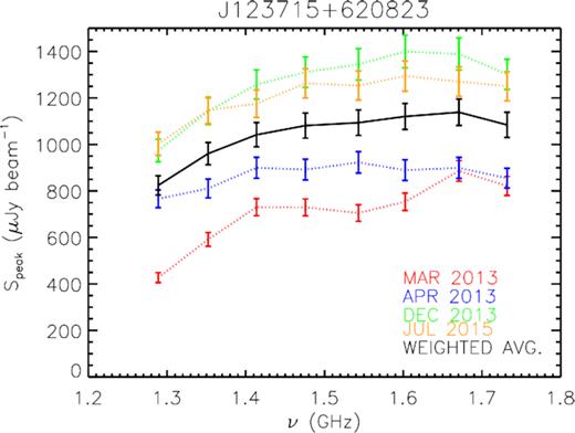
Peak flux densities in eight frequency intervals across four epochs (2013 March–2015 July) for the e-MERLIN variable unresolved source J123715+620823. Due to small gain errors in the data, it was necessary to iteratively self-calibrate (‘peel’) this bright (∼105 times the noise level at the centre of the field) point source epoch-by-epoch using a multifrequency sky model. After peeling, we reinjected the source back in to our uv data using the sensitivity-weighted average flux in each spectral window (solid black line).
2.5 Wide-field integrated imaging with e-MERLIN and VLA
The primary goal of e-MERGE is to obtain high surface brightness sensitivity (|$\sigma _{\rm 1.5\, GHz}\lesssim 5\, \mu$|Jy arcsec−2) imaging at sub-arcsecond resolution across a field of view that is large enough (≳15 × 15 arcmin2) to allow a representative study of the high-redshift radio source population. This combination of observing goals is beyond the capabilities of either e-MERLIN or VLA individually, hence the combination of data from VLA and e-MERLIN is essential.
While co-addition of data sets obtained at different times from different array configurations of the same telescope (e.g. VLA, ALMA, ATCA) is a routine operation in modern interferometry, the differing internal frequency/polarization structures of our new e-MERLIN/VLA and previously published MERLIN/VLA data sets prohibited a straightforward concatenation of the data sets using standard (e.g. |$\cal AIPS$|dbcon or casaconcat) tasks.
Historically, circumventing this issue has necessitated either image-plane combination of data sets, or further re-mapping of the internal structures of the uv data sets to allow them to be merged.
The former approach involves generating dirty maps (i.e. with no cleaning/deconvolution) from each data set independently, co-adding them in the image plane, and then deconvolving the co-added map using the weighted average of the individual PSFs using the Högbom (1974) clean algorithm, as implemented in the |$\cal AIPS$| task apcln (e.g. Muxlow et al. 2005). While this approach sidesteps difficulties in combining inhomogeneous data sets properly in the uv plane – and produces reliable results for sources whose angular sizes are in the range of scales to which both arrays are sensitive (θ ∼ 1–1.5 arcsec) – the fidelity of the resulting image is subject to the reliance on purely image-based deconvolution using ‘minor cycles’ only. This is a potentially serious limitation when imaging structures for which only one array provides useful spatial information (i.e. extended sources which are resolved out by e-MERLIN or compact sources which are unresolved by VLA), where cleaning using a hybrid beam is not the appropriate thing to do.
An alternative approach – used by Biggs & Ivison (2008) – is to collapse the multifrequency data sets from each telescope along the frequency axis, preserving the uvw coordinates of each visibility (as was done for the pre-2010 VLA data described in Section 2.3), and then concatenate and image these single-channel data sets. This approach allows the uv coverage of multiple data sets to be combined, bypassing the issues with image-plane combination and allowing a single imaging run to be performed utilizing the Schwab (1984) clean algorithm (i.e. consisting of both major and minor clean cycles). However, while this approach has proved successful when combining together MERLIN/VLA data sets of relatively modest bandwidth, the technique of collapsing the available bandwidth down to a single frequency channel implicitly assumes that the source spectral index is flat across the observed bandwidth. While this condition is approximately satisfied for most sources given the narrow bandwidths of the older MERLIN/VLA data sets, it cannot be assumed given the orders of magnitude increase in bandwidth which is now available with both instruments. For sources with non-flat spectral indexes, this approach would introduce amplitude errors in the final image.
In order to successfully merge our (e)MERLIN and old/new VLA data sets we use wsclean (Offringa et al. 2014), a fast, wide-field imager developed for imaging data from modern synthesis arrays. wsclean utilizes the |$w$|-stacking algorithm, which captures sky curvature over the wide FoV of e-MERLIN by modelling the radio sky in three dimensions, discretising the data along a vector |$w$| (which points along the line of sight of the array to the phase centre of the observations), performs a Fourier Transform on each |$w$|-layer and finally recombines the |$w$|-layers in the image plane. In addition to offering significant performance advantages over the casa implementation of the |$w$|-projection algorithm (for details, see Offringa et al. 2014), wsclean also possesses the ability to read in multiple calibrated Measurement Sets from multiple arrays (with arbitrary frequency/polarization setups) and grid them on-the-fly, sidestepping the difficulties we encountered when trying to merge these data sets using standard |$\cal AIPS$|/casa tasks. wsclean allows us to generate deep, wide-field images using all the 1–2 GHz data from both arrays (spanning a 20-yr observing campaign) in a single, deep imaging run, deconvolving the resulting (deterministic) PSF from the image using both major and minor cycles, and without loss of frequency or polarization information.
2.5.1 Data weights
The e-MERGE survey was conceived with the aim that – upon completion – the naturally weighted combined-array 1.5-GHz image would yield a PSF that could be well characterized by a 2D Gaussian function, with minimal sidelobe structure. In this survey description paper for DR1, we present imaging which utilizes ∼90 per cent of the anticipated VLA 1.5-GHz data volume, but with only ∼25 per cent of the e-MERLIN observations included. As a result, the PSF arising from our naturally weighted combined data set more closely resembles the superposition of two 2D Gaussian components – one, a narrow (θres ∼ 0.2 arcsec) component representing the e-MERLIN PSF, and the other, a broader (θres ∼ 1.5 arcsec) component representing the VLA A-array PSF – joined together with significant shoulders at around ∼50 per cent of the peak.3
Standard clean techniques to deconvolve the PSF from an interferometer dirty image entail iteratively subtracting a scaled version of the true PSF (the so-called ‘dirty beam’) at the locations of peaks in the image, building a model of delta functions (known as ‘clean components’), Fourier transforming these into the uv plane and subtracting these from the data. This process is typically repeated until the residual image is noise like, before the clean components are restored to the residual image by convolving them with an idealized (2D Gaussian) representation of the PSF. The flux density scale of the image is in units of Jy beam−1, where the denominator is derived from the volume of the fitted PSF. While this approach works well for images where the dirty beam closely resembles a 2D Gaussian to begin with, great care must be taken if the dirty beam has prominent shoulders. In creating our cleaned naturally weighted (e)MERLIN plus VLA combination image, we subtracted scaled versions of the true PSF at the locations of positive flux and then restored these with an idealized Gaussian, whose fit is dominated by the narrow central portion of the beam produced by the e-MERLIN baselines. The nominal angular resolution of this naturally weighted combination image is θres = 0.28 × 0.26 arcsec2, with a beam position angle of 84° , and the image has a representative noise level of |$\sigma _{\rm 1.5\, GHz}=1.17\, \mu$|Jy beam−1. However, subsequent flux density recovery tests comparing the VLA-only and the e-MERLIN+VLA combination images revealed that while this process works well for bright, compact sources, (recovering ∼100 per cent of the VLA flux density but with ∼5 times higher angular resolution), our ability to recover the flux density in fainter, more extended (≳0.7 arcsec) sources is severely compromised. This is because the representative angular resolutions of the clean component map and the residual image (on to which the restored clean components are inserted) are essentially decoupled (due to the restoring beam being a poor fit to the ‘true’, shouldered PSF). As a result of this, faint radio sources restored at high resolution are imprinted on ∼ arcsecond noise pedestals, containing the residual un-cleaned flux density in the map. This limits the ability of source-fitting codes to find the edges of faint radio sources in the naturally weighted image, with a tendency to artificially boost their size and flux density estimates. Moreover, the difference in the effective angular resolutions of the clean component and residual images renders the map units themselves (Jy beam−1) problematic. This issue will be discussed in more detail in the forthcoming e-MERGE catalogue paper (Thomson et al., in preparation), however, we stress that, in principle, it applies to any interferometer image whose dirty beam deviates significantly from a 2D Gaussian.
To mitigate this effect, a further two 1.5-GHz combined-array images were created with the aim of smoothing out the shoulders of the naturally weighted e-MERLIN+VLA PSF. We achieved this by using the wsclean implementation of ‘Tukey’ tapers (Tukey 1962). Tukey tapers are used to adjust the relative contributions of short and long baselines in the gridded data set, and work in concert with the more familiar Briggs (1995) robust weighting schemes. They can be used to smooth the inner or outer portions of the uv plane (in units of λ) with a tapered cosine window which runs smoothly from 0 to 1 between user-specified start (UVm) and end points (iTT).4 By effectively down-weighting data on certain baselines, the output image then allows a different trade-off between angular resolution, rms sensitivity per beam, and dirty beam Gaussianity to be achieved.
To provide optimally sensitive imaging of extended |$\mu$|Jy radio sources while retaining ∼kpc-scale (i.e. sub-arcsecond) resolution, we complement the naturally weighted e-MERLIN+VLA combination image with two images which utilize Tukey tapers:
We create a maximally sensitive combination image using both inner and outer Tukey tapers (UVm = 0λ and iTT = 82240λ) along with a briggs robust value of 1.5. The angular resolution of this image is θres = 0.89 × 0.78 arcsec2 at a position angle of 105° and with an rms sensitivity |$\sigma _{\rm 1.5\, GHz}=1.71\, \mu$|Jy beam−1 (corresponding to |${\sim}2.46\, \mu$|Jy arcsec−2).
To exploit the synergy between our 1.5 5.5 GHz data sets (and thus to enable spatially resolved spectral index work), we have identified a weighting scheme which delivers a 1.5-GHz PSF that is close to that of the VLA 5.5-GHz mosaic image of Guidetti et al. (2017). We find that a combination of a Briggs taper with robust=1.5 and a Tukey taper with UVm = 0λ, iTT = 164480λ yields a 2D Gaussian PSF of size θres = 0.55 × 0.42 arcsec2 at a position angle of 112°. To provide an exact match for the 5.5-GHz PSF (θres = 0.56 × 0.47 arcsec2 at a position angle of 88°) we use this weighting scheme in combination with the –beam-shape parameter of wsclean. The resulting rms of this image is |$\sigma _{\rm 1.5\, GHz}=1.94\, \mu$|Jy beam−1 or |${\sim}7.37\, \mu$|Jy arcsec−2.
Together with VLA-only and e-MERLIN-only images (representing the extremes of the trade-off in sensitivity and resolution), these constitute a suite of five 1.5-GHz images that are optimized for a range of high-redshift science applications (see Table 3).
e-MERGE DR1 image summary.
| Image name | Description | Frequency | Synthesized beam | |$\sigma _{\rm rms}^a$| |
|---|---|---|---|---|
| (μJy beam−1) | ||||
| VLA | Naturally weighted | 1.5 GHz | 1.68 × 1.48 arcsec2 @ |$105{^{\circ}_{.}}88$| | 2.04 |
| Combined (Max. Sens.) | e-MERLIN + VLA combined-array image, | 1.5 GHz | 0.89 × 0.78 arcsec2 @ 105○ | 1.71 |
| weighted for improved sensitivity | ||||
| Combined (PSF Match) | e-MERLIN + VLA, weighted to match VLA | 1.5 GHz | 0.56 × 0.47 arcsec2 @ 88○ | 1.94 |
| 5.5-GHz resolution for spectral index work | ||||
| Combined (Max. Res.) | e-MERLIN + VLA, weighted for | 1.5 GHz | 0.28 × 0.26 arcsec2 @ 84○ | 1.17 |
| improved angular resolution | ||||
| e-MERLIN | e-MERLIN-only, naturally weighted | 1.5 GHz | 0.31 × 0.21 arcsec2 @ 149○ | 2.50 |
| C-band mosaic | 5.5 GHz, naturally weighted mosaicb | 5.5 GHz | 0.56 × 0.47 arcsec2 @ 88○ | 1.84 |
aσrms values are in units of |$\mu$|Jy beam−1, and are therefore dependent on the beam size – the ‘max res’ combination image has the lowest σrms (and therefore, the best point-source sensitivity of all images in this data release), however, the small beam limits its sensitivity to extended emission, to which the lower resolution combined-array images – with slightly higher σrms – are more sensitive.
bPreviously published by Guidetti et al. (2017).
The trade-off in angular resolution versus sensitivity between these five weighting schemes is highlighted for a representative subset of e-MERGE sources in Fig. 6.
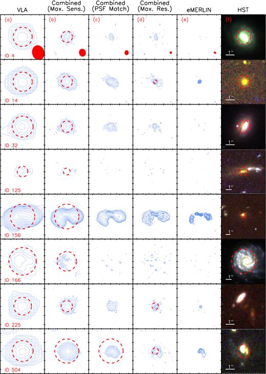
Thumbnail images of eight representative sources (one per row) from the e-MERGE DR1 catalogue of 848 radio sources (Thomson et al., in preparation), highlighting the need for a suite of radio images made with different weighting schemes (each offering a unique trade-off between angular resolution and sensitivity) to fully characterize the extragalactic radio source population. Columns (a)–(e) step through the five e-MERGE DR1 1.5-GHz radio images in order of increasing angular resolution from VLA-only to e-MERLIN-only (see Table 3 for details). Contours begin at 3σ and ascend in steps of |$3\sqrt{2}\times \sigma$| thereafter, and the fitted Petrosian size (if statistically significant) is shown as a red-dashed circle (see Section 3.4). Column (f) shows three-colour (F606W, F814W, F850LP) HST CANDELS thumbnail images for each source, with the optical Petrosian size shown as a red dashed circle. A 1.0-arcsec scale bar is shown in white in each colour thumbnail. Together, columns (a)–(f) highlight the diversity of the e-MERGE DR1 source population, including a mixture of core-dominated AGN within quiescent host galaxies (ID 14), merger-driven star-forming galaxies (ID 125, 225), high-redshift wide-angle tail AGN (ID 156), and face-on spiral galaxies (ID 166).
2.5.2 Primary beam corrections for combined-array images
The primary beam response of a radio antenna defines the usable FoV of a single-pointing image made with that antenna. In the direction of the pointing centre, the primary beam response is unity, dropping to ∼50 per cent at the half-power beamwidth (θHPBW ∼ λ/D for an antenna diameter D). For wide-field images, it is essential to correct the observed flux densities of sources observed off-axis from the pointing centre for this primary beam response.
In the case of homogeneous arrays (such as VLA), the primary beam response of the array is equivalent to that of an individual antenna. Moreover, because the antennas are identical, the primary beam response of the array is invariant to the fraction of data flagged on each antenna/baseline. Detailed primary beam models for the VLA in each antenna/frequency configuration are incorporated in casa and can be implemented on-the-fly during imaging runs by setting pbcor=True in tclean, or can be exported as fits images using the widebandpbcor task. However, for inhomogeneous arrays (such as e-MERLIN) the primary beam response is a sensitivity-weighted combination of the primary beam responses from each antenna pair in the array. These weights are influenced by the proportion of data flagged on each antenna/baseline, and thus vary from observation to observation.
To correct our e-MERLIN observations for the primary beam response, we constructed a theoretical primary beam model based on the weighted combination of the primary beams for each pair of antennas in the array. This model is presented in detail in Wrigley (2016) and Wrigley et al. (in preparation), however, we provide an outline of our approach here. To model the primary beam of e-MERLIN, we first derived theoretical 2D complex voltage patterns |$V_i V^{\star }_j$| and |$V^{\star }_i V_j$| for each pair of antennas ij based on knowledge of the construction of the antennas (effective antenna diameters, feed blocking diameters, illumination tapers, pylon obstructions and spherical shadow projections due to the support structures for the secondary reflector). We checked the fidelity of these theoretical voltage patterns via holographic scans, wherein each pair of antennas in the array was pointed in turn at a bright point source (e.g. 3C 84), with one antenna tracking the source while the other scanned across it in a raster-like manner, nodding in elevation and azimuth to map out the expected main beam.
This primary beam model comprises a 2D array representing the relative sensitivity of our e-MERLIN observations as a function of position from the pointing centre; the model is normalized to unity at the pointing centre, and tapers to ∼57 per cent at the corners of our DR1 images, a distance of ∼11 arcmin from the pointing centre. We applied this primary beam correction to the images made using wsclean in the image plane, dividing the uncorrected map by the beam model.
To construct an appropriate primary beam model for our e-MERLIN + VLA combination images, we exported the 2D VLA primary beam model from casa, re-gridded it to the same pixel scale as our e-MERLIN beam model and then created sensitivity-weighted combinations of the e-MERLIN + VLA primary beam for each of the DR1 images listed in Table 1. We again applied these corrections by dividing the wsclean combined-array maps by the appropriate primary beam model.
The effect of applying these primary beam models is an elevation in the noise level (and in source flux densities) in the corrected images as a function of distance from the pointing centre, which is highlighted in Fig. 4.
2.5.3 Time and bandwidth smearing
As discussed in 2.1, the quantization of astrophysical emission by an interferometer into discrete time intervals and frequency channels results in imprecisions in the (u, |$v$|) coordinates of the recorded data with respect to their true values. Both time and frequency quantization have the effect of distorting the synthesized image in ways that cannot be deconvolved analytically using a single, spatially invariant deconvolution kernel. The effect is a ‘smearing’ of sources in the image plane, which conserves their total flux densities but lowers their peak flux densities. Time/bandwidth smearing are an inescapable aspect of creating images from any interferometer, but the effects are most significant in wide-field images, particularly on longer baselines and for sources located far from the pointing centre (e.g. Bridle & Schwab 1999).
In order to compress the data volume of e-MERGE and ease the computational burden of imaging, we averaged our e-MERLIN observations by a factor of 4 times (from a native resolution of 0.125 MHz/channel to 0.5 MHz/channel), but did not average the data in time beyond the 1 s/integration limit of the e-MERLIN correlator. We did not average the VLA observations in frequency beyond the native 1 MHz/channel resolution, but did average in time to 3 s/integration (as described in Section 2.2).
Using the SimuCLASS interferometry simulation pipeline developed by Harrison et al. (2020), we empirically determine that on the longest e-MERLIN baselines, at a distance of 10.6 arcmin from the pointing centre, bandwidth smearing induces a drop in the peak flux density of a point source of up to |${\sim}20{{\ \rm per\ cent}}$|. This result – which is in agreement with the analytical relations in Bridle & Schwab (1999) – limits the usable field-of-view of these data to the 15 × 15 acmin2 region overlying the HST CANDELS region of GOODS-N. By including the shorter baselines of the VLA, this smearing is reduced significantly, to: (i) ∼4 per cent in the VLA-only image5; and (ii) |${\lesssim}8{{\ \rm per\ cent}}$| at the edges of the ‘maximum sensitivity’ DR1 combination image.
The frequency averaging of our e-MERLIN observations – which was necessary in order to image the data using current compute hardware – is therefore the primary factor limiting the usable e-MERGE DR1 FoV to that of the 76-m Lovell Telescope. We note that in order to fully image the e-MERLIN observations out to the primary beam of the 25-m antennas (as is planned for e-MERGE DR2) it will be necessary to re-reduce these data with no frequency averaging applied.
2.5.4 VLA 5.5 GHz
Included in the e-MERGE DR1 release is the seven-pointing VLA 5.5-GHz mosaic image of GOODS-N centred on J2000 RA |$12^{h}36^{m}49{.\!\!\!\!^{{\rm {\small {s}}}}}4$| and Dec. +62○12′58|${^{\prime\prime}_{.}}$|0, which was previously published by Guidetti et al. (2017, in which a detailed description of the data reduction and imaging strategies is presented). For completeness, these observations are briefly summarized below.
The GOODS-N field was observed at 5.5 GHz with the VLA in the A- and B-configuration, for 14 and 2.5 h, respectively. The total bandwidth of these observations is 2 GHz, comprised 16 spws of 64 channels each (corresponding to a frequency resolution of 2 MHz/channel).
These data were reduced using standard |$\cal AIPS$| techniques, with the bright source J1241+6020 serving as the phase reference source and with 3C 286 and J1407+2828 (OQ 208) as flux density and bandpass calibrators, respectively. Each pointing was imaged separately using the casa task tclean, using the multiterm, multifrequency synthesis mode (mtmfs) to account for the frequency dependence of the sky model. These images were corrected for primary beam attenuation using the task widebandpbcor and then combined in the image plane to create the final mosaic using the |$\cal AIPS$| task hgeom, with each pointing contributing to the overlapping regions in proportion to the local noise level of the individual images. The final mosaic covers a 13.5-arcmin diameter area with central rms of Jy beam−1, and has a synthesized beam θres = 0.56 × 0.47 arcsec2 at a position angle of 88 deg.
A total of 94 AGN and star-forming galaxies were extracted above 5σ, of which 56 are classified as spatially extended (see Guidetti et al. 2017, for details).
2.6 Ancillary data products
2.6.1 VLA 10 GHz
To provide additional high-frequency radio coverage of a subset of the e-MERGE DR1 sources, we also use observations taken at 10 GHz as part of the GOODS-N Jansky VLA Pilot Survey (Murphy et al. 2017). These observations (conducted under the VLA project code 14B-037) comprise a single deep pointing (24.5 h on source) towards |$\alpha =12^{\rm h}36^{\rm m}51{.\!\!\!\!^{{\rm {\small {s}}}}}21$|, δ = +62○13′37|${^{\prime\prime}_{.}}$|4, with approximately 23 h of observations carried out with the VLA in A-array and 1.5 h in C-array. We retrieved these data from the VLA archive and, following Murphy et al. (2017), calibrated them using the VLA casa pipeline (included with casa|$v$| 4.5.1). 3C 286 served as the flux and bandpass calibrator source and J1302+5728 was used as the complex gain calibrator source.
We created an image from the reduced uv data with wsclean using natural weighting, which includes an optimized version of the multiscale deconvolution algorithm (Cornwell 2008; Offringa & Smirnov 2017) to facilitate deconvolution of the VLA beam from spatially xtended structures. Our final image covers the VLA X-band primary beam (6 arcmin in diameter) down to a median rms sensitivity of |$\sigma _{\rm 10\, GHz}=1.28\, \mu$|Jy beam−1 across the field (reaching |$\sigma _{\rm 10\, GHz}=0.56\, \mu$|Jy beam−1 within the inner (0.8 × 0.8 arcsec2) and with a restoring beam that is well approximated by a 2D Gaussian of size 0.27 × 0.23 arcsec2 at a position angle of 4°.
2.6.2 Optical–near-IR observations
In order to derive key physical properties (e.g. photometric/spectroscopic redshift information and stellar masses) of the host galaxies associated with the e-MERGE DR1 sample, we utilize the rich, multiwavelength catalogue of the GOODS-N field compiled by the 3D-HST team (Brammer et al. 2012; Skelton et al. 2014). This includes seven-band HST imaging from the 3D-HST, CANDELS (Grogin et al. 2011; Koekemoer et al. 2011) and GOODS (Giavalisco et al. 2004) projects, along with a compilation of ancillary data from the literature including: (i) Subaru Suprime-Cam B, V, Rc, Ic, |$z$|′ and Kitt Peak National Observatory 4-m telescope U-band imaging from the Hawaii–HDFN project (Capak et al. 2004); (ii) Subaru MOIRCS J, H, K imaging from the MODS project (Kajisawa et al. 2011), and (iii) Spitzer IRAC 3.6-, 4.5-, 5.8-, 8.0-μm imaging from the GOODS and SEDS projects (Dickinson et al. 2003; Ashby et al. 2013).
We defer a detailed discussion of the multiwavelength properties of the e-MERGE sample to future papers, but emphasize that the 3D-HST catalogue is used to provide photometric redshift information for the e-MERGE sample in the following sections.
3 ANALYSIS, RESULTS, AND DISCUSSION
The detailed properties (and construction) of the e-MERGE DR1 1.5-GHz source catalogue will be presented in detail in a forthcoming publication (Thomson et al., in preparation), however, we present an overview of the catalogue properties here, including the 1.5-GHz angular size measurements of ∼500 star-forming galaxies and AGN at |$z$| ≳ 1.
3.1 Radio source catalogue
For the purposes of this survey description paper, we use the VLA 1.5-GHz image to identify sources, as this image has the optimal surface brightness sensitivity to detect sources, which are extended on the scales expected of high-redshift galaxies (≳0.5 arcsec); we then measure the sizes and integrated flux densities of these VLA-identified sources in the higher resolution 1.5-GHz maps.
We find that the source catalogue has a Purity of 0.993 (i.e. a false-positive rate |${\le}1{{\ \rm per\ cent}}$|) at a source detection threshold of 4.8σ.
After visually inspecting the data, best-fitting model and residual thumbnails for each extracted source, we found evidence that some sources exhibited significant residual emission, which was not well fit, indicating that the morphologies of some sources are too complicated (even in the 1|${^{\prime\prime}_{.}}$|5 resolution VLA image) to be adequately modelled with Gaussian components alone. To improve the model accuracy, we re-ran the source extraction procedure with the atrous_do module enabled within pybdsf. This module decomposes the residual image left after multicomponent Gaussian fitting in to wavelet images in order to identify extended emission – essentially ‘mopping up’ the extended flux from morphologically complex sources – and was used to produce the final VLA 1.5-GHz flux density measurements for our e-MERGE DR1 source catalogue.
3.2 Illustrative analysis of a representative high-redshift e-MERGE source
To highlight the science capabilities of our high angular resolution (sub-arcsecond) e-MERGE DR1 data set, we present a short, single-object study of a representative source from our full catalogue of 848 sources. J123634+621241 (ID 504 in our catalogue, hereafter referred to as ‘The Seahorse Galaxy’ on account of its 1.5-GHz radio morphology) is an extended source (LAS = 1.0 arcsec), the brightest component of which overlies the highly dust-obscured nuclear region of an i = 22.3 mag merging S cd galaxy at |$z$| = 1.224 (Barger et al. 2014). We measure total flux densities of |$S_{\rm 1.5\, GHz}=174.0\pm 5.6\, \mu$|Jy and |$S_{\rm 5.5\, GHz}=46.2\pm 4.8\, \mu$|Jy, respectively, using our resolution-matched 1.5 - and 5.5-GHz maps, from which we find that the Seahorse has a low-frequency spectral index, which is consistent with aged synchrotron emission (|$\alpha ^{\rm 5.5\, GHz}_{\rm 1.5\, GHz}=-1.02\pm 0.08$|).
The Seahorse is the most likely radio counterpart to the SCUBA 850-µm source, HDF 850.7 (Serjeant et al. 2003). We show e-MERGE radio images of this source in Fig. 7. The total stellar mass of the merging system is estimated from SED-fitting to be |$(9.5\pm 0.1)\times 10^{10}\, \mathrm{M_{\odot }}$| (Skelton et al. 2014). The extended radio emission of the Seahorse overlies two bright optical components running to the south into a tidal tail. Combining our resolution-matched 1.5- and 5.5-GHz maps, we create a spectral index map for the Seahorse, measuring a moderately steep (α ∼ −0.7) spectral index across the bright component, which steepens to α ∼ −1.0 as the extended radio component follows the red tail of the merging system.
![Thumbnail images of the interacting system J123634+621241, dubbed the ‘Seahorse’ galaxy. (a) HST three-colour (F606W, F814W, F850LP) image highlighting the disturbed morphology of this apparent close pair of merging galaxies. The green-dotted circle has a radius of 1.5 arcsec, representing the VLA 1.5-GHz PSF. (b) 1.5–5.5-GHz spectral index ($\alpha ^{\rm 5.5\, GHz}_{\rm 1.5\, GHz}$) image for the Seahorse (red heatmap) with cyan contours beginning at 3 × σ (and in steps of $\sqrt{2}\times \sigma$ thereafter for a local $\sigma =2.9\, \mu$Jy beam−1) showing the 1.5-GHz morphology in the PSF-matched e-MERLIN+VLA combination image (i.e. the 1.5-GHz image with the same beam as the 5.5-GHz VLA-only mosaic image, and which is used to create the spectral index image). The spectral index, $\alpha ^{\rm 5.5\, GHz}_{\rm 1.5\, GHz}$ ranges between $-1.0 \lt \alpha ^{\rm 5.5\, GHz}_{\rm 1.5\, GHz}\lt -0.1$. We see evidence that the redder optical galaxy is associated with steep spectrum (α < −1.0) aged synchrotron emission in the radio tail, whilst the bluer optical galaxy is coincident with younger, less-steep (α ∼ −0.7) radio emission found in the bright extended nuclear starburst. The 0.56 × 0.47 arcsec2PSF is shown in the bottom right-hand corner with a cyan ellipse. (c) e-MERLIN-only 1.5-GHz contours of the Seahorse galaxy, plotted in magenta at $[-1,1,2,3,4,6...12]\times 5.925\, \mu$Jy beam−1 (i.e. $2.5\times \sigma _{\rm 1.5\, GHz}$) over the monochrome HST F814W optical image. The peak of the radio emission likely traces the optically obscured nuclear starburst which is responsible for producing the far-IR emission in this system. The 0.31 × 0.21 arcsec2e-MERLIN PSF is shown. (d) VLA 10 GHz contours of the Seahorse galaxy (Murphy et al. 2017) plotted in red over the monochrome HST F814W image. The 0.27 × 0.23 arcsec2 PSF is shown. Contours begin at 3 × σ and in steps of thereafter for Jy beam−1. At these higher radio frequencies, there is very little extended emission visible from the evolved stellar population and instead we see redshifted free–free emission which directly traces the current active starburst.](https://oup.silverchair-cdn.com/oup/backfile/Content_public/Journal/mnras/495/1/10.1093_mnras_staa1279/3/m_staa1279fig7.jpeg?Expires=1749961569&Signature=FC~3~ajTnv4RuSCh~4dT2D2Hlyc4gqPcaIuGjSUCgoXGcIqwvXAbkMy5KVCp8urEf3ySbo5GyJrGpkd38~KmvnhP9X6pd3LFKncys8SFJl-OWMkPjGUPO5TTVQ07jvhvbQ4xitpLxxMuihzhf5cj1vfuGyxZqjOce~00crSbtMjQNoYrnRZUlsjFnf45VfE3Ld25TU7Ct8IVU8yvT1WDF7HrT3G0iiPaN5hoLGY6D55a-ElvvauoLrEQXX947HHs1mIQ0Ifxq4~~YlERI7HO1TsAFdNXJ1IDGMCgNYa9jNCbCrHNCMzNxkMhiBfWLHJppPfyTDQI4kFgAXqrXmLTSw__&Key-Pair-Id=APKAIE5G5CRDK6RD3PGA)
Thumbnail images of the interacting system J123634+621241, dubbed the ‘Seahorse’ galaxy. (a) HST three-colour (F606W, F814W, F850LP) image highlighting the disturbed morphology of this apparent close pair of merging galaxies. The green-dotted circle has a radius of 1.5 arcsec, representing the VLA 1.5-GHz PSF. (b) 1.5–5.5-GHz spectral index (|$\alpha ^{\rm 5.5\, GHz}_{\rm 1.5\, GHz}$|) image for the Seahorse (red heatmap) with cyan contours beginning at 3 × σ (and in steps of |$\sqrt{2}\times \sigma$| thereafter for a local |$\sigma =2.9\, \mu$|Jy beam−1) showing the 1.5-GHz morphology in the PSF-matched e-MERLIN+VLA combination image (i.e. the 1.5-GHz image with the same beam as the 5.5-GHz VLA-only mosaic image, and which is used to create the spectral index image). The spectral index, |$\alpha ^{\rm 5.5\, GHz}_{\rm 1.5\, GHz}$| ranges between |$-1.0 \lt \alpha ^{\rm 5.5\, GHz}_{\rm 1.5\, GHz}\lt -0.1$|. We see evidence that the redder optical galaxy is associated with steep spectrum (α < −1.0) aged synchrotron emission in the radio tail, whilst the bluer optical galaxy is coincident with younger, less-steep (α ∼ −0.7) radio emission found in the bright extended nuclear starburst. The 0.56 × 0.47 arcsec2PSF is shown in the bottom right-hand corner with a cyan ellipse. (c) e-MERLIN-only 1.5-GHz contours of the Seahorse galaxy, plotted in magenta at |$[-1,1,2,3,4,6...12]\times 5.925\, \mu$|Jy beam−1 (i.e. |$2.5\times \sigma _{\rm 1.5\, GHz}$|) over the monochrome HST F814W optical image. The peak of the radio emission likely traces the optically obscured nuclear starburst which is responsible for producing the far-IR emission in this system. The 0.31 × 0.21 arcsec2e-MERLIN PSF is shown. (d) VLA 10 GHz contours of the Seahorse galaxy (Murphy et al. 2017) plotted in red over the monochrome HST F814W image. The 0.27 × 0.23 arcsec2 PSF is shown. Contours begin at 3 × σ and in steps of thereafter for Jy beam−1. At these higher radio frequencies, there is very little extended emission visible from the evolved stellar population and instead we see redshifted free–free emission which directly traces the current active starburst.
The Seahorse also lies within the GOODS-N Jansky VLA 10 GHz Pilot Survey area (Murphy et al. 2017). Only the brightest component seen by e-MERLIN at 1.5 GHz is detected at 10 GHz, overlying the optically obscured region and suggesting that the extended radio emission in the e-MERLIN-only image (whose 0.31 × 0.21 arcsec2 PSF is similar to the 0.27 × 0.23 arcsec2 PSF of the 10-GHz image) is the result of dust-obscured, spatially extended star formation rather than the blending of compact cores from the two progenitor galaxies in this merging system (Fig. 7). Murphy et al. (2017) measure a flux density for the Seahorse of |$S_{\rm 10\, GHz}=36.71\pm 0.06\, \mu$|Jy. The 5.5–10-GHz spectral index is therefore |$\alpha ^{\rm 10\, GHz}_{\rm 5.5\, GHz}=-0.38\pm 0.25$|, which is considerably flatter than the 1.5–5.5-GHz spectral index measured previously, and is consistent with spectral flattening due to increasing thermal emission at higher frequencies.
Our interpretation of the radio structure in the Seahorse is therefore that it is dominated by intense star formation taking place within the very dusty regions of the merging system which produces obscuration and reddening in the optical bands. This radio emission, in turn, likely traces the regions from which the prodigious far-IR luminosity originates, owing to the FIRRC. The brightest component, which is detectable from 1.5–10 GHz appears to have a flatter radio spectrum (due to the increased spatial density of H ii regions) than the surrounding material, which is undetected at 10 GHz (and hence likely has a steeper spectrum tracing a synchrotron halo around the central starburst).
The Seahorse galaxy system illustrates the advantages of high angular resolution imaging at ∼GHz radio frequencies, where the older radio emitting plasma is more easily detected than at higher frequencies due to its spectral properties. Observing at νobs ≳ 10 GHz with the VLA provides the required resolution to resolve such systems, but suffers from strong spectral selection effects which must be understood and disentangled before meaningful comparisons with samples selected in the GHz-window can be made.
3.3 The redshift and luminosity distributions of e-MERGE DR1 sources
To provide added value to the e-MERGE DR1 catalogue, we match our radio source list to the multiband optical/IR catalogue of HST WFC3-selected sources compiled by the 3D-HST team (Skelton et al. 2014). To check the astrometric accuracy of the 3D-HST catalogue, we take the VLA source positions of the brightest 100 radio sources common to both the e-MERGE DR1 survey region and 3D-HSTHST WFC3 mosaic images, and stack in each of the F105W, F125W, and F160W images at these source positions. We fit the stacked images with a 2D Gaussian and measure the offsets in the fitted centroids from the centre of the thumbnail images (which are centred on the VLA source positions). We measure small (δθ≲ 0.2 arcmin) linear offsets in RA. To correct for this, we apply a linear shift to the 3D-HST catalogue in RA, corresponding to the mean offset (δθ = 0.12672 arcmin).
With this shift applied, we find optical counterparts to 587 of our 848 VLA-detected e-MERGE sources (69 per cent) within an ∼1.5-arcsec error circle, providing redshift information and allowing both the luminosities and linear sizes of our radio-selected sample to be measured. Of the 261 e-MERGE DR1 sources without optical counterparts, 235 were found to lie outwith the footprint of the HST F125W image, which defines the survey area of 3D-HST (Skelton et al. 2014). There are therefore 26 e-MERGE sources detected above 4.8σ at 1.5 GHz which lie within the 3D-HST survey area and which do not have counterparts in the 3D-HST source catalogue, an optical non-detection rate of |$4.2{{\ \rm per\ cent}}$|.
To establish whether these 26 optically blank radio sources are real or spurious, we extract thumbnail images at their measured radio positions in the VLA 1.5 GHz and 5.5 GHz radio images (cf. Beswick et al. 2008) and HST F775W (I-band) and SubaruK-band near-IR images, and stack the 26 thumbnail images in each waveband using a median stacking algorithm (e.g. Thomson et al. 2017). The stacked thumbnail images are shown in Fig. 8. By fitting Gaussian source components to the two stacked radio thumbnails using the casa task imfit we measure median radio flux densities of |$S_{\rm 1.5\, GHz}=29\pm 1\, \mu$|Jy and |$S_{\rm 5.5\, GHz}=11\pm 3\, \mu$|Jy. To measure median AB magnitudes from the stacked optical thumbnails, we perform aperture photometry in Source Extractor (Bertin & Arnouts 1996) using a 1.5 arcsec aperture and zero-point offsets of 25.671 (Skelton et al. 2014) and 26.0 (Kajisawa et al. 2011) for the HST F775W I-band and SubaruK-band images, respectively. We measure median magnitudes of K = 24.01 ± 0.62 and I = 26.07 ± 2.33. We detect significant emission in the four stacked thumbnail images, confirming that on average the 26 optically undetected e-MERGE sources are real, albeit faint and red: K ∼ 24 and (I − K) = 2.06 ± 0.19. This combination of radio flux densities and optical colours is consistent with emission from high-redshift (|$z$| > 2) dust-obscured star-forming galaxies which are frequently missed in even the deepest optical studies (e.g. Smail 2002).
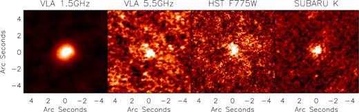
Stacked thumbnail images of 26 e-MERGE DR1 sources with VLA 1.5-GHz detections above 4.8 × σ, but no reported optical counterparts in the 3D-HST catalogue of Skelton et al. (2014). We fit the radio emission in the two-stacked radio thumbnail images using Gaussian source components, measuring flux densities of |$S_{\rm 1.5\, GHz}=29\pm 1\, \mu$|Jy and |$S_{\rm 5.5\, GHz}=11\pm 3\, \mu$|Jy, and measure I- and K-band magnitudes of I = 26.07 ± 2.33 and K = 24.01 ± 0.62 via HST F775W and SubaruK-band imaging from Skelton et al. (2014) and Kajisawa et al. (2011), respectively. The detection of emission in all four stacked thumbnails highlights that the 26 e-MERGE sources which lack counterparts in the 3D-HST optical catalogue are (on average) real sources, associated with red ((I − K) = 2.06 ± 0.19), faint (K ∼ 24) host galaxies.
To provide an independent check of our data reduction, imaging and cataloguing strategies, we compare the e-MERGE DR1 VLA source flux densities against those reported in the VLA GOODS-N catalogue of Owen (2018), whose analysis was based on an independent reduction of the same raw telescope data. Our imaging strategy differs from that used by Owen (2018) in terms of data weights and imaging algorithms used (e.g. Owen 2018, uses the casatclean package with multicale clean, |$w$|-projection and a Briggs robust value of 0.5, whereas we use wsclean with |$w$|-stacking and natural weighting). Moreover, the fields of view of the two VLA images differ slightly: Owen (2018) images a circular field 18 arcmin in diameter, and achieves a noise level near the centre of the field of |$\sigma _{\rm 1.5\, GHz}=2.2\mu$|Jy beam−1 from 39 h of observations, detecting 795 radio sources down to 4.5 × σrms. As previously discussed (Section 2.3), the e-MERGE DR1 survey area is a 15 × 15 arcmin2, and by including both the Owen (2018, post-upgrade) and Richards (2000, preupgrade) VLA observations in our imaging run, we achieve a noise level of |$\sigma _{\rm 1.5\, GHz}=2.04\, \mu$|Jy beam−1 at the centre of the field. Of the 795 sources in the Owen (2018) catalogue, 664 lie within the e-MERGE DR1 survey area. In turn, 812/848 e-MERGE DR1 sources lie within the footprint of the Owen (2018) catalogue. We cross-match the Owen (2018) and e-MERGE DR1 source catalogues using a 1|${^{\prime\prime}_{.}}$|5 matching radius (corresponding to the VLA 1.5-GHz synthesized beam), finding 602 sources in common. This implies that within the area common to both studies there are 17 e-MERGE DR1 sources, which are not in the Owen (2018) catalogue, and 62 radio sources in the Owen (2018) catalogue which are not in the e-MERGE DR1 catalogue. However, this 62 includes 24 extended (>2–3 arcsec) sources which visual inspection confirmed are in fact in the e-MERGE catalogue, albeit with recorded source positions (determined by pybdsf) which are >1.5 arcsec away from the position determined by the |$\cal AIPS$|sad routine used by Owen (2018). The remaining 38 sources are relatively low significance (〈S/N〉 = 5.2) detections in the Owen (2018) catalogue, and the differing imaging and source identification strategies used may be enough to explain their non-detections in e-MERGE. We show a comparison between the Owen (2018) and e-MERGE DR1 VLA integrated flux densities of 602 sources in Fig. 9. We perform a linear least-squares fit to these flux densities, measuring |$\log _{10}(S_{\rm 1.5\, GHz; Owen}/\mu {\rm Jy}) = 0.946\times \log _{10}(S_{\rm 1.5\, GHz; eMERGE}/\mu {\rm Jy}) + 0.079$|. We believe this modest excess of flux in the e-MERGE catalogue with respect to the catalogue of Owen (2018) can be partly explained by the different source-fitting methodologies: the sad routine in |$\cal AIPS$| used by Owen (2018) fits Gaussian models to detected source components using a least-squares method, whereas (as previously discussed) the atrous_do module in pybdsf supplements this source-fititng with a wavelet decomposition module to capture the residual emission around extended sources, which is not accounted for by Gaussian source fitting alone. The sum of the integrated flux densities of these 602 sources in the e-MERGE DR1 catalogue is 45.83 mJy, 3.8 per cent higher than the sum of the integrated flux densities of the same sources in the Owen (2018) catalogue (44.15 mJy). The median flux densities of these 602 sources, however, are |$30.7\pm 1.6$| and |$30.0\pm 1.1\, \mu$|Jy in e-MERGE DR1 and the catalogue of Owen (2018), respectively, which are consistent within the measurement errors. We therefore conclude that there are no significant offsets in our overall flux scale with respect to Owen (2018), and that our source catalogues are consistent to within the overall flux scale calibration uncertainties of the VLA.6
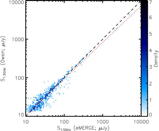
Flux density comparison between radio source components detected in the VLA 1.5-GHz study of Owen (2018) and those detected in our independent reduction and analysis of the same observations. We show our results as a density plot, with 2D bins of width |$\log _{10}(S_{\rm 1.5\, GHz}/\mu {\rm Jy})=0.025$|. A colour bar on the right-hand side of the plot indicates the number of sources in each flux bin. We show the one-to-one relation as a dashed black line, along with the log-linear best fit, |$S_{\rm 1.5\, GHz, Owen} = 0.95S_{\rm 1.5\, GHz, eMERGE}+0.08$|, which is shown as a dotted red line. We have a tendency to measure slightly higher flux densities for our source components with respect to the flux densities presented in the catalogue of Owen (2018); we believe this result is due to the source-fitting methodology of pybdsf, which uses wavelet decomposition to ‘mop up’ extended emission which is not well fit by Gaussian source components.
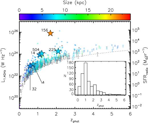
Main panel: The luminosity–redshift plane for e-MERGE DR1, including the 587 radio-detected sources with optical counterparts within 1.5 arcsec from the 3D-HST catalogue (Skelton et al. 2014). We measure rest-frame |$L_{\rm 1.4\, GHz}$| from our observed-frame 1.5-GHz flux densities using this redshift information, along with: (i) the measured radio spectral index (|$\alpha ^{\rm 5.5\, GHz}_{\rm 1.5\, GHz}$|) for sources detected in both e-MERGE bands; (ii) α = −0.8 for sources which are non-detected at 5.5 GHz (provided that spectral index is consistent with the 5.5 -GHz non-detection); (iii) α < −0.8, if required by the corresponding |$3\times \sigma _{\rm 5.5\, GHz}$| upper limits. To illustrate our sensitivity to SFR as a function of redshift, we use the 1.4 GHz to SFR conversion factor of Murphy et al. (2011), which highlights our ability to detect high-SFR systems at high-redshift (i.e. SFR ∼ 100–1000 M⊙ yr−1 at |$z$| ∼ 2.5). Points are colour-coded by the fitted radio sizes (if measured; see Section 3.4), with sources which lack a significant size measurement coloured in charcoal. We highlight six of the illustrative sources shown in Fig. 6 with large star symbols. Inset: The photometric redshift distribution of e-MERGE DR1 peaks at 〈|$z$|〉 = 1.08 ± 0.04, with a tail (accounting for |${\sim}15{{\ \rm per\ cent}}$| of the sample) lying between |$z$| = 2.0–5.6 (Skelton et al. 2014).
For sources detected at both 1.5 and 5.5 GHz, we k-correct using the measured radio spectral index, |$\alpha ^{\rm 5.5\, GHz}_{\rm 1.5\, GHz}$|, and for sources detected at 1.5 GHz but not at 5.5 GHz we use either α = −0.8 (if consistent with the 5.5-GHz non-detection), or a steeper spectral index if required by the |$3\times \sigma _{\rm 5.5\, GHz}$| upper limit.
While we emphasize that it is highly unlikely that any radio-selected galaxy sample at high-redshift will be entirely dominated by star formation, we see in Fig. 10 that the e-MERGE DR1 maps are sufficiently sensitive to detect radio emission from a combination of AGN and high-SFR systems, such as SMGs (SFR ∼ 100–1000 M⊙ yr−1), at least out to |$z$| ∼ 2.5. For |$z$| ≳ 3, the strong positive k-correction in the radio bands biases our flux-limited 1.5-GHz sample towards radio sources, which are an order of magnitude more luminous than typical SMGs; these high-power, high-redshift radio systems are almost certainly an AGN-dominated population. We defer detailed classification of the e-MERGE radio source population to future publications.
3.4 The radio sizes of SFGs and AGN from z = 1–3
To measure the (sub-arcsecond) resolved radio properties of e-MERGE DR1 sources, we use the VLA source catalogue to provide positional priors and then measure the Petrosian radii (RP; following Petrosian 1976; Wrigley 2016) of these sources in the higher resolution combined-array e-MERLIN + VLA and e-MERLIN-only images. We define RP as the radius r at which the local surface brightness profile, I(R), equals 0.4 times the mean surface brightness within RP, 〈I〉R (e.g. Graham et al. 2005).
As discussed in Section 2.5, the suite of five e-MERGE 1.5-GHz DR1 images offers a sliding scale in both angular resolution and surface brightness sensitivity between the extremes of VLA-only and e-MERLIN-only imaging. To provide a set of representative source size measurements for our high-redshift galaxy sample, we focus our analysis on the e-MERLIN + VLA ‘Maximum Sensitivity’ image (Table 3). This image has an angular resolution of 0.89 × 0.78 arcsec and an rms sensitivity of |$\sigma _{\rm rms}=1.71\, \mu$|Jy beam−1, (corresponding to a linear scale of ∼7 kpc and a 3σ point source SFR sensitivity of 15 M⊙ yr−1 beam−1 at |$z$| = 1, using equation 5). This image is thus well suited to providing canonical size measurements for star-forming galaxies at high redshift, whose typical optical angular sizes are ∼5–10 kpc (Williams et al. 2010; van der Wel et al. 2014; Rujopakarn et al. 2016).
We measure the uncertainties on the individual Petrosian size estimates using a Monte Carlo process, wherein for each source, for each annulus we perturb every pixel by a value drawn from a Gaussian distribution of fluxes whose width is equal to the local rms, and re-fit the profile. We repeat this process 100 times per annulus, and define the ±1σ error on the fitted size, which results from this process for each source from the range of minimum/maximum Petrosian sizes allowed by this process. These size errors – along with profiles for each source – will be presented along with the source catalogue in a forthcoming publication (Thomson et al., in preparation).
In order to provide a consistent comparison between the radio and optical size distributions, we smooth the HST CANDELS F606W, F814W, and F850LP images to match the resolution of the maximum-sensitivity e-MERGE image, and then co-add these images in order to provide a high S/N, broad-band optical image. We then fit Petrosian optical sizes using the same methodology as was employed in our radio imaging. We show the size histograms from fitting to our radio and stacked optical images in Fig. 11. Of the 587 e-MERGE DR1 sources with optical counterparts in the 3D-HST catalogue, 312 both have the photometric redshift information needed to derive linear source sizes, and yield convergent Petrosian size measurements in both the radio and the optical bands. The remaining 275 sources either lack a photometric redshift measurement, have too little S/N to fit a resolved profile in one or both images, or lie within crowded fields, and hence I(R) > 0.4 × 〈I〉R for all physically plausible sizes (i.e. ≲50 kpc).
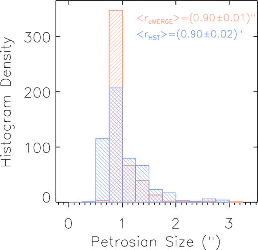
Histogram of optical and radio angular sizes of e-MERGE sources. From our parent catalogue of 848 VLA 1.5-GHz-detected sources, we measure deconvolved radio Petrosian sizes for 479 galaxies (56 per cent of the sample) and deconvolved optical sizes (from a stacked three-band HST CANDELS F606W, F814W, and F850LP image, smoothed to match the 0.8-arcsec beam of our e-MERGE ‘maximum sensitivity’ radio image) for 525 galaxies (62 per cent of the sample). Galaxies without size measurements include optically blank radio sources (3 per cent), and sources whose size measurements are consistent with being up-scattered point sources (either because the light profiles of these sources are noise-like, or because they lie within a few arcseconds of a much brighter source, and the Petrosian size cannot be disentangled from the blended light profile: 35 per cent). The median 1.5-GHz radio and optical sizes in e-MERGE are 〈re-MERGE〉 = 0.90 ± 0.01 arcsec and and 〈rHST〉 = 0.90 ± 0.0201 arcsec, respectively. Note that these histograms include sources both with and without photometric redshift information from the 3D-HST catalogue.
To test whether these 312 deconvolved size measurements represent real source structure, or whether they represent spurious fitting of point sources, we create a simulated image (with Gaussian noise) and inject 20,000 point sources with S/N ratios between 0 < S/N < 20, and then convolve this with the combination image dirty beam. We then perform Petrosian size fitting on this simulated image at the positions of the known point sources. Unsurprisingly, we find that lower S/N point sources have a greater tendency to be up-scattered in size than higher S/N point sources. Following Bondi et al. (2008) and Thomson et al. (2019), we parameterize this size ‘up-scattering’ as a function of S/N by measuring the envelope in size versus S/N below which 99 per cent of the simulated point sources lie. We determine that |${\lesssim}1{{\ \rm per\ cent}}$| of point sources scatter above an envelope of log (RP/arcsec) = −1.05log (S/N) − 0.25. Applying this envelope to the Petrosian size measurements derived from our real data, we find that 64/312 source sizes are consistent with being unresolved at 0.7-arcsec resolution. The remaining 248 sources represent the largest high-redshift galaxy sample to date with resolved kpc-scale size measurements at 1.5 GHz: This sample is poised to expand with our forthcoming, deeper, wider-area DR2 data release.
We show a comparison between the radio and optical Petrosian sizes of these 248 e-MERGE galaxies in Fig. 12. The mean radio-to-optical size ratio of sources detected in both images is 1.02 ± 0.03 – where the uncertainty quoted is the standard error (i.e. |$\sigma /\sqrt{n}$|) – implying that the radio emission traces the rest-frame UV stellar light. Splitting this sample near the median radio luminosity (|$L_{\rm 1.4\, GHz}\sim 1.4\times 10^{23}$| W Hz−1) we measure a radio-to-optical size ratio of 1.04 ± 0.05 for the fainter half of the sample and 1.00 ± 0.04 for the brighter half. The median radio sizes are 7.7 ± 0.2 and 6.7 ± 0.1 kpc above and below the median luminosity, respectively. This increase in radio size with radio luminosity is consistent with the findings of Bondi et al. (2018), whose study on the size evolution of the 3-GHz-selected VLA-COSMOS sample (Smolčić et al. 2017) uncovered similar behaviour for both the radio-loud AGN and radio-quiet AGN in their sample. Our near-unity radio-to-optical size ratio is in tension with a results from the VLA COSMOS 3 GHz study (Jiménez-Andrade et al. 2019), whose median radio size is ∼1.3–2 times smaller than the optical/UV continuum emission which traces the stellar component. Given that the VLA COSMOS 3 GHz and e-MERGE 1.5-GHz maximum sensitivity images are of comparable angular resolution (θCOSMOS = 0.75 arcsec, cf. θe-MERGE = 0.84 arcsec), it is unlikely this discrepancy in radio-to-optical size ratios is a result of resolution effects, but rather reflects real differences in the physical scales of processes emitting at different radio frequencies. As previously suggested by Murphy et al. (2017) and Thomson et al. (2019), these differences may include frequency-dependent cosmic-ray diffusion and/or may be due to the increasing thermal fraction at higher rest-frame radio frequencies, revealing time lags between the production of free–free and synchrotron emission in star-forming galaxies (e.g. Bressan et al. 2002; Thomson et al. 2014; Gómez-Guijarro et al. 2019).
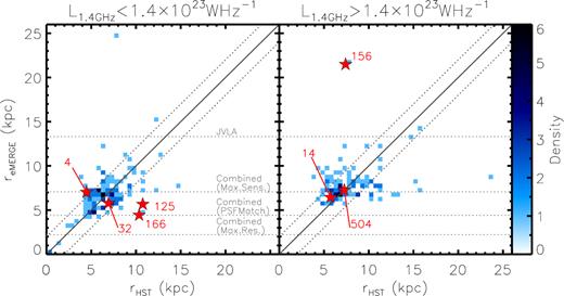
The deconvolved radio and rest-frame optical size distribution of 248 e-MERGE radio sources with Petrosian size measurements and photometric redshift information from the 3D-HST survey (Skelton et al. 2014). Linear radio sizes are measured from our ‘Maximum Sensitivity’ combined-array image, which has an angular resolution of ∼0.8 arcsec, and optical sizes are measured from a stacked three-band (F606W, F814W, F850LP) HST CANDELS image, after smoothing to the same resolution as our radio map. The distribution of linear sizes is shown as two density plots, in bins of width 0.5 × 0.5 kpc2, with horizontal lines showing the effective linear size of the PSFs of the suite of e-MERGE images at the median redshift of the sample (<|$z$| > =1.08 ± 0.04). e-MERGE allows us for the first time to measure the angular sizes of ‘normal’ galaxies at |$z$| ∼ 1 at 1.5 GHz, revealing a mean radio-to-optical size ratio of 1.02 ± 0.03. Large star symbols represent the individual sources in Fig. 6 for which both radio and optical size measurements are available. Left-hand panel: e-MERGE radio versus HST optical sizes for 124 galaxies below the median radio luminosity of the sample (|$L_{\rm 1.4\, GHz}\lt 1.4\times 10^{23}$| W Hz−1). The density plot peaks around a median 1.04 ± 0.05, based on a radio size of re-MERGE = 6.74 ± 0.23 kpc and optical size of rHST = 6.45 ± 0.20 kpc. Right-hand panel: radio versus optical size density plot for the brighter half of the sample (|$L_{\rm 1.4\, GHz}\gt 1.4\times 10^{23}$| W Hz−1). The median e-MERGE-to-optical size ratio for brighter radio sources is 1.00 ± 0.04, based on a radio size re-MERGE = 7.73 ± 0.19 kpc and optical size of rHST = 7.73 ± 0.27. In both subsamples, therefore, the radio emission appears to trace similar scales to the optical stellar light, suggesting a source population, which is not dominated by jetted radio AGN. At higher radio powers there is weak evidence (∼1σ) of a lower radio-to-optical size ratio than at weaker radio powers, which may be indicative of a radio source population in which compact nuclear AGN emission begins to play a more prevalent role.
In total, 20 sources (∼8 per cent of the 248 e-MERGE galaxies with fitted optical and radio size information) have radio-to-optical size ratios, which exceed 1.2. These include ID 156, a wide-angle tailed radio source associated with a compact red elliptical host galaxy. There are 21 galaxies (∼8 per cent of the sample with size information), which have radio-to-optical size ratios smaller than 0.8. These include ID 166, a face-on spiral galaxy with radio emission tracing star formation down one of the spiral arms only (see Fig. 6 for details).
Recently, Lindroos et al. (2018) used the uv-stacking technique combined with Sérsic model fitting (with a fixed n = 1) to measure the optical and radio size evolution of optically selected star-forming galaxies from |$z$| = 0–3 across a stellar mass range M⋆ ∼ 1010.5−1011 M⊙ using the (pre-2010) MERLIN and VLA GOODS-N data which are included as part of e-MERGE DR1. Lindroos et al. (2018) found that the median radio sizes become larger at lower redshift, and that they are on average ∼2 times smaller both than the optical sizes of the same stacked samples, and than the Hα sizes of typical star-forming galaxies. They concluded that radio continuum emission therefore preferentially traces morphologically compact star formation, concentrated towards the centres of galaxies. We do not see this trend among the 248 e-MERGE sources for which we can measure accurate sizes in our maximum-sensitivity combination image (see Fig. 10). However, we note that the PSF of this maximum-sensitivity combination image – at half the size of the VLA-only PSF – still only marginally resolves structures which are ∼6 kpc in size at |$z$| ≳ 1, and that around 49 per cent of our optically detected sample do not have reliable size measurements in this map. If the radio emission in high-redshift galaxies is significantly more compact than even the ∼0.8-arcsec beam of our e-MERGE maximum sensitivity image, then we may see evidence of size-evolution in the higher resolution (but lower surface brightness) e-MERGE DR1 images in future publications.
4 CONCLUSIONS
In this paper, we have described the motivation, design, data reduction, and imaging strategies underpinning e-MERGE, a large legacy project combining e-MERLIN and VLA data at 1.5 and 5.5 GHz (along with previously obtained but newly re-processed observations from the pre-2010 MERLIN and VLA instruments). e-MERGE combines the long baseline capabilities of e-MERLIN with the high surface brightness sensitivity of the VLA to form a unique deep-field radio survey capable of imaging and studying the |$\mu$|Jy radio source population (i.e. star-forming galaxies and AGN at |$z$| ≳ 1) at sub-arcsecond angular resolution with high surface brightness sensitivity (|$\sigma _{\rm 1.5\, GHz}\sim 1.5\, \mu$|Jy beam−1).
We have presented a description of the procedure for modelling the complicated e-MERLIN primary beam, described post-processing steps, which we applied to our data to correct for the deliterious effects of strongly variable unresolved sources within our target field, and described the imaging strategies necessary to seamlessly combine e-MERLIN and VLA data in the uv plane in order to better the capabilities of either telescope individually.
We have shown some early science results from e-MERGE, including an analysis of the redshifts, radio luminosities, and/or linear sizes of ∼500 cosmologically distant radio-selected sources. Our redshift distribution peaks at 〈|$z$|〉 = 1.08 ± 0.04, with a tail (|${\sim}15{{\ \rm per\ cent}}$| of the sample) lying at redshifts |$z$| = 2–5.6. The sensitivity of e-MERGE DR1 is such that both AGN and starburst galaxies (SFR = 102–103 M⊙ yr−1) are expected to be found in large numbers out to at least |$z$| ∼ 3. We have highlighted the ability of e-MERGE to spatially resolve high-redshift star-forming galaxies via an analysis of a |$z$| = 1.2 dust-obscured SMG detected in three radio frequency bands (1.5, 5.5 and 10 GHz). We see evidence for significant size evolution in this source across the three-frequency bands, with the 1.5-GHz emission tracing scales roughly twice as large as those traced at 10 GHz at comparable resolution.
This is intended as the first in a series of publications, which will explore the full scientific potential of our suite of sensitive, high-resolution 1.5- and 5.5-GHz images of the GOODS-N field as probes of star formation and AGN activity in high-redshift source populations.
ACKNOWLEDGEMENTS
APT, TWBM, RJB, and MAG acknowledge support from STFC (ST/P000649/1). APT further acknowledges and thanks Robert Dickson, Peter Draper, David Hempston, Anthony Holloway, and Alan Lotts for their extensive support managing the high-performance computing infrastructure, which has been essential for the successful delivery of e-MERGE DR1. JFR acknowledges the financial assistance of the South African Radio Astronomy Observatory (SARAO) towards this research (http://sarao.ac.za). IP acknowledges support from INAF under the PRIN SKA/CTA project ‘FORECaST’ and the PRIN MAIN STREAM project ‘SAuROS’. EI acknowledges partial support from FONDECYT through grant no 1171710. We thank the anonymous reviewer for their detailed and constructive referee report, which has undoubtedly improved the quality of the final manuscript. e-MERLIN is a National Facility operated by the University of Manchester at Jodrell Bank Observatory on behalf of STFC. The National Radio Astronomy Observatory is a facility of the National Science Foundation operated under cooperative agreement by Associated Universities, Inc. The authors acknowledge the use of the IRIDIS High Performance Computing Facility, and associated support services at the University of Southampton, in the completion of this work. We thank IRIS (www.iris.ac.uk) for provision of high-performance computing facilities. STFC IRIS is investing in the UK’s Radio and mm/sub-mm Interferometry Services in order to improve data quality and throughput. The European VLBI Network is a joint facility of independent European, African, Asian, and North American radio astronomy institutes. Scientific results from data presented in this publication are derived from the following EVN project code(s): EG078B. The research leading to these results has received funding from the European Commission Horizon 2020 Research and Innovation Programme under grant agreement no. 730562 (RadioNet).
Footnotes
e-MERGE is an e-MERLIN legacy survey, and therefore exists to produce lasting legacy data and images for the whole astronomical community. An e-MERGE DR1 source catalogue will be released in a forthcoming publication. After a short proprietary period, the full suite of e-MERGE DR1 wide-field images will be made available to the community. We encourage potential external collaborators and other interested parties to visit the e-MERGE website for the latest information: http://www.e-merlin.ac.uk/legacy-emerge.html
By removing these sources from the uv data, we avoid the need to clean them during deconvolution, significantly reducing the area to be imaged (and thus the computational burden) without loss of information on the target field.
It is expected that the inclusion of ∼4 time more e-MERLIN data in e-MERGE DR2 will smooth out the shoulders of the naturally weighted combined PSF and achieve our long-term goal of a Gaussian PSF.
See https://sourceforge.net/p/wsclean/wiki/Tapering/ for details.
In agreement with the performance specification of the VLA: https://science.nrao.edu/facilities/vla/docs/manuals/oss/performance/fov
