


ABSTRACT
We used magnetohydrodynamical cosmological simulations to investigate the cross-correlation between different observables (i.e. X-ray emission, Sunyaev–Zeldovich (SZ) signal at 21 cm, H i temperature decrement, diffuse synchrotron emission, and Faraday Rotation) as a probe of the diffuse matter distribution in the cosmic web. We adopt a uniform and simplistic approach to produce synthetic observations at various wavelengths, and we compare the detection chances of different combinations of observables correlated with each other and with the underlying galaxy distribution in the volume. With presently available surveys of galaxies and existing instruments, the best chances to detect the diffuse gas in the cosmic web outside of haloes is by cross-correlating the distribution of galaxies with SZ observations. We also find that the cross-correlation between the galaxy network and the radio emission or the Faraday Rotation can already be used to limit the amplitude of extragalactic magnetic fields, well outside of the cluster volume usually explored by existing radio observations, and to probe the origin of cosmic magnetism with the future generation of radio surveys.
1 INTRODUCTION
Galaxy surveys and numerical simulations have consistently shown that the large-scale structure of the Universe is organized in a hierarchy of highly overdense haloes, mildly overdense filaments, and underdense voids. A large fraction of the baryonic matter (around 50 per cent) should indeed reside in the form of plasma in such cosmic web, at densities 10–100 times the average cosmic value and temperature mostly of 105–107 K, forming the warm–hot intergalactic medium (WHIM, Cen & Ostriker 1999).
The detection and the characterization of the WHIM in cosmic filaments is of primary interest. First, finding in the WHIM the missing baryonic mass (e.g. Nicastro 2016) would verify one of the pillars of modern cosmological structure formation paradigm. Its distribution would trace the geometry and define the topology of the Universe (e.g. Cautun et al. 2014). Furthermore, filaments evolve with adiabatic physics (besides gravity) driving the gas dynamics, but with other physical processes possibly influencing their chemical (e.g. Martizzi et al. 2019) and magnetic (e.g. Gheller & Vazza 2019) properties. Thanks to a less violent growth compared to galaxy clusters, they preserve essential information on the original environment in which structure formation takes place, besides on magnetogenesis and primordial magnetism.
Observing the WHIM has been so far a challenge at all wavelengths (e.g. Dietrich et al. 2012; Nevalainen et al. 2015; Connor et al. 2018, 2019), due to its extremely low particle density, leading to a faint emission at the limit or below the current instrumental sensitivity, which is also strongly affected by background/foreground contributions and observational noise and artefacts. Only since recently imaging of the WHIM, connected to massive nearby galaxy clusters (Eckert et al. 2015) or to dense protoclusters at high redshift (Umehata et al. 2019), has become feasible. A few additional potential detections of filaments around cosmic structures have been reported, using the Sunyaev–Zeldovich (SZ) effect (e.g. Planck Collaboration VIII 2013; Tanimura et al. 2019a) or radio waves (e.g. Botteon et al. 2018; Vacca et al. 2018; Govoni et al. 2019). More recently, Tanimura et al. (2019b) and de Graaff et al. (2019) have presented the possible first detection of the coldest part of the coldest part of the WHIM in the cosmic web, by stacking the thermal SZ signal of pairs of galaxies or pairs of galaxy groups.
Statistical techniques can be adopted to detect the presence of the cosmic web, overcoming the limits of current instruments. In this work, we will rely on the cross-correlation analysis to measure the signatures of large-scales diffuse emission considering various ‘mass tracers’ (galaxies, X-ray emission, radio emission, etc.). Cross-correlation is a widely used methodology in signal and image processing, that we will exploit in order to identify faint signals, below the sensitivity of single instruments. In fact noise and, generally speaking, artefacts and background/foreground affecting different types of observation are completely unrelated from each other and, in general, from the signal, hence their combination tends to cancel out. On the other hand, actual signals coming from the same source tend to sum constructively and magnify.
Many examples of successful applications of the cross-correlation analysis in astronomy can be found, the following list far from being exhaustive. The method has been first used to detect the integrated Sachs–Wolfe effect in cosmic microwave background (CMB) data (e.g. Nolta et al. 2004). Hurier, Singh & Hernández-Monteagudo (2019) detected the cross-correlation between X-rays and CMB weak lensing, as well as performed autocorrelation and cross-correlation of SZ, X-rays, and weak lensing to assess the galaxy cluster hydrostatic mass bias. Singh et al. (2016) investigated the detectability of the cross-correlation between galaxy distribution, SZ and X-ray for various future surveys and with the goal of detecting the circumgalactic medium, estimating a maximum detection efficiency for |$\sim 10^{13} \, \mathrm{M}_{\odot }$| haloes at z ∼ 1–2. Muñoz & Loeb (2018) proposed the detection of the WHIM by cross-correlating the dispersion measure of fast radio bursts and thermal SZ maps, which is now a concrete possibility thanks to the deployment of dedicated instruments for fast radio burst (e.g. CHIME). Moving to higher redshift, Ma et al. (2018) computed the amplitude of the cross-correlation signal between the emission from the energetic and high-z source of X-ray background and the H i signal from intergalactic gas the epoch of reionization.
In the radio domain, cross-correlation has been adopted to detect faint, spatially correlated, emission below the noise limit of radio surveys. Vernstrom et al. (2017) and Brown et al. (2017) have presented first attempts of cross-correlating the distribution of radio emission in the continuum to that of galaxies in large portions of the sky, seeking for a positive correlation between diffuse emission and the cosmic web. Vernstrom et al. (2017) cross-correlated early MWA observations at 169 MHz with the distribution of galaxies in the WISE and 2MASS galaxy surveys, for a 22 × 22 deg2field of view. Brown et al. (2017) used instead 2.3-Ghz observations from the S-PASS survey, and cross-correlated them with template radio emission from a constrained MHD simulation. In both cases, no significant detection of a cross-correlation was found, probably due to the limited sensitivity and spatial resolution of radio data (as well as due to the possible contamination of unresolved radiogalaxies, whose clustering properties correlate with that of the galaxy distribution). However, upper limits on the average amplitude of magnetic fields in the cosmic web in the range |$B \le 0.01\!-\!0.1 \,\rm \mu G$| were derived from both works.
Being a statistical methodology, the cross-correlation has the limitation that it provides no direct inference of the underlying matter distribution and of the physical mechanisms behind the detected signal. Proper modelling is necessary to link the observed statistics to the properties of the corresponding sources.
Numerical simulations represent the most effective and general tool to pursue such objective. We have exploited a number of magnetohydrodynamical (MHD) simulations run by our group, encompassing a broad variety of magnetic, astrophysical, and galaxy evolution setup to create a variety of mock observations. From the simulations, in fact, different types of signals (synchrotron, SZ, X...) can be calculated and correlated with each other or with the DM, representative of the galaxy distribution. The mock observations have been generated with or without the contribution of additional noise. The latter allows to better discriminate between different prescriptions for the gas physics and its magnetic properties. Random noise has been added to images considering the typical detection threshold of several instruments in the relevant energy bands. We have considered both instruments ‘currently’ available, meaning that they are already operational (like ASKAP or LOFAR-HBA) or they will be in the next future (like eROSITA), and ‘future’ instruments, that will become available on a longer time horizon (like SKA or ATHENA-WFI). The former points out the expected detection with data immediately available, the latter the possible improvements in the long-term perspective.
The resulting simulated data set has then be used to perform a first systematic survey of the degree of cross-correlation measured between several relevant observable signatures of the diffuse gas in the cosmic web. Such survey is intended both to guide future studies adopting the cross-correlation statistics to detect the WHIM in various kind of observations, and to interpret possible detections in terms of the properties of the underlying diffuse gas component. We present a first example of such kind of interpretation, by comparing the cross-correlation measured between galaxies and synchrotron emission in our different models with the results obtained by Vernstrom et al. (2017).
Our paper is organized as follows. The numerical methods used for the cosmological simulations and to generate the multiwavelengths mock observations will be described in Section 2. In the same section, we will also validate the different models assessing their reliability for the performed analysis. In Section 3, we will give an essential introduction to cross-correlation and its usage on the simulated images. In Section 4, the results of applying the cross-correlation analysis to the different models will be presented and discussed. Conclusions will be drawn in Section 5.
2 SIMULATIONS AND MOCK OBSERVATIONS
2.1 Numerical simulations
Our simulations adopted the cosmological Eulerian code enzo (Bryan et al. 2014), with a fixed mesh resolution. The code has been customized by our group mainly with the purpose of including different mechanisms for the seeding of magnetic fields in cosmology, as explained in detail in Vazza et al. (2017) and Gheller & Vazza (2019).
The MHD solver used in our simulations implements the conservative Dedner formulation (Dedner et al. 2002), which utilizes hyperbolic divergence cleaning to keep the |$\nabla \cdot \boldsymbol {B}$| as small as possible, and the piecewise linear method reconstruction technique with fluxes calculated using the Harten–Lax–Van Leer approximate Riemann solver. Time integration is performed using the total variation diminishing second-order Runge–Kutta scheme (Shu & Osher 1988). We used the GPU-accelerated MHD version of enzo by Wang, Abel & Kaehler (2010), which gives an approximately four time speedup compared to the more standard CPU version of enzo in the 10243 uniform grid runs used here. The constant spatial resolution has the advantage of providing the best-resolved description of magnetic fields even in low-density regions, which would typically go unrefined by adaptive mesh refinement approaches.
We have exploited a subset of data extracted from the ‘Chronos++suite’1, which in total includes 24 different models, designed to explore various plausible scenarios for the origin and evolution of extragalactic magnetic fields (Vazza et al. 2017). Here, we focus on three models: primordial, dynamo, and astrophysical scenarios (see also Table 12):
Primordial model: A non-radiative simulation in which we assumed the existence of a volume-filling magnetic field at the beginning of the simulation, with magnitude B0 = 1 nG. This simulation represents our ‘baseline’ reference model for the cosmic web.
Dynamo model: Also a non-radiative simulation as before, in which we estimated at run-time via sub-grid modelling the small-scale dynamo amplification of very weak seed field of primordial origin (|$B_0 = 10^{-9}\, \rm nG$|). Here, the dissipation of solenoidal turbulence into magnetic field amplification is estimated on the fly by extrapolating the information resolved at our fixed |$83.3 \,\rm kpc$| cell resolution. In this work, we consider model ‘DYN5’ of Gheller & Vazza (2019), which gives a reasonable match to the magnetic field strength in galaxy clusters.
Astrophysical model: A more sophisticated simulation including radiative gas cooling, chemistry, star formation, and thermal/magnetic feedback from (a) stellar activity and/or (b) feedback by supermassive black holes (SMBH), simulated at run time using prescriptions available in enzo (e.g. Kravtsov 2003; Kim et al. 2011; Bryan et al. 2014). Our reference model here, ‘CSFBH2’, assumes accretion for SMBH following from the spherical Bondi–Hoyle formula with a fixed |$0.01 \,\rm M_{\odot }\,yr^{-1}$| accretion rate, and a fixed ‘boost’ factor to the mass growth rate of SMBH (αBondi = 1000) to balance the effect of coarse resolution, properly resolving the mass accretion rate on to our simulated SMBH particles. We have extended enzo coupling thermal feedback to the injection of additional magnetic energy via bipolar jets, with an efficiency with respect to the feedback energy computed at run-time, ϵSF, b and ϵBH, b for the stellar and SMBH, respectively. Here, we used |$\epsilon _{\rm SF,b}=10$| and |$1{{\ \rm per\ cent}}$| for the magnetic feedback, while for the feedback efficiency (referred to the |$\epsilon _{\rm SF, BH} = \dot{M} c^2$| energy accreted by star-forming or black hole particles) we used 10−8 and 0.01, respectively. This run gives a good match to the observed cosmic average star formation rate (SFR) as well as to observed galaxy cluster scaling relations (as discussed in Section 2.3 and in Vazza et al. 2017). The implementation of cooling adopted here follows the non-equilibrium evolution of primordial (metal-free) gas. The chemical rate equations are solved using a semi-implicit backward difference scheme, while heating and cooling processes include a number of processes (e.g. atomic line excitation, recombination, collisional excitation, free–free transitions, Compton scattering of the CMB and photoionization from metagalactic UV backgrounds). The species that are tracked at run-time in the simulation are only atomic species (i.e. H, H+, He, He+, He++, and electrons), and their evolution is computed by solving the rate equations with one Jacobi iteration with implicit Eulerian time discretization, with a coupling between thermal and chemical states at subcylces in the hydrodynamical time-step (see Bryan et al. 2014, and references therein for more details).
Main parameters of the three runs in the Chronos++suite used in the present work. From the left- to right-hand columns define the presence of radiative cooling or star-forming particles, the critical gas number density n* to trigger star formation in the Kravtsov (2003) model, the time-scale for star formation t*, the thermal feedback efficiency, and the magnetic feedback efficiency (ϵSF and ϵSF, b) from star-forming regions; the efficiency of Bondi accretion αBondi in the Kim et al. (2011) model for SMBH; the thermal feedback efficiency and the magnetic feedback efficiency (ϵBH and ϵBH, b) from SMBH; the intensity of the initial magnetic field, B0; the presence of sub-grid dynamo amplification at run time; the ID of the run and some additional descriptive notes. All simulations evolved a |$85^3\, \rm Mpc^3$| volume using 10243 cells and DM particles, starting at redshift z = 38. The name convention of all runs is consistent with Vazza et al. (2017).
| Cooling | Star | n* | t* | ϵSF | ϵSF, b | αBondi | ϵBH | ϵBH, b | B0 | Dynamo | ID | Description |
|---|---|---|---|---|---|---|---|---|---|---|---|---|
| formation | (1 cm-3) | (Gyr) | (G) | |||||||||
| No | No | – | – | – | – | – | – | – | 10−9 | No | Baseline | Primordial, uniform, |
| No | No | – | – | – | – | – | – | – | 10−18 | |$10 \cdot \epsilon _{\rm dyn}(\mathcal {M})$| | DYN5 | Low primordial, efficient dynamo |
| Yes | Yes | 0.0001 | 1.5 | 10−8 | 0.01 | 103 fix. | 0.05 | 0.01 | 10−18 | – | CSFBH2 | Star formation, BH, constant |$(\frac{0.01 \, \mathrm{M}_{\odot }}{\rm yr})$| |
List of observable properties and adopted detection threshold.
| Observable | Frequency/en.range | Instrument | Detection threshold | Note |
|---|---|---|---|---|
| X-ray emission | 0.3–2.0 keV | eROSITA | |$\approx \!2 \times 10^{-15} \rm erg\, s^{-1} \,cm^2$| | 10 ks (polar region survey) |
| X-ray emission | 0.3–2.0 keV | ATHENA-WFI | |$\approx \!5 \times 10^{-16} \rm erg\, s^{-1} \,cm^2$| | 100 ks |
| Differential H i Temperature | 1400 MHz | ASKAP | |$\approx \!10^{-3} \rm \,K$| | Possum |
| Differential H i Temperature | 1000 MHz | SKA-MID | |$\approx \!10^{-5} \rm \,K$| | Phase II survcey |
| Radio emission | 200 MHz | LOFAR-HBA | |$\approx \!1.0 \rm\, \mu Jy\, arcsec^{-2}$| | Tier I survey |
| Radio emission | 200 MHz | SKA-LOW | |$\approx \!0.2 \rm \, \mu Jy\, arcsec^{-2}$| | 2 years survey |
| Radio emission | 180 MHz | MWA | |$\approx \!0.28 \rm \, \mu Jy\, arcsec^{-2}$| | MWA Phase I |
| Faraday Rotation | 1400 MHz | ASKAP/Meerkat | |$\approx \!1\, \rm rad\, m^{-2}$| | Possum/Mightee-Pol |
| Faraday Rotation | 1000 MHz | SKA-MID | |$\approx \!0.1\, \rm rad\, m^{-2}$| | Phase II |
| Compton Y-param. | 220 GHz | PLANCK | ≈2890 | |
| Compton Y-param. | 21 GHz | AtlAS | ≈1000 |
Note: We associate to each observable a reference instrument, which loosely corresponds to the adopted observational cut.
All the runs adopted the Lambda cold dark matter (ΛCDM) cosmology, with density parameters ΩBM = 0.0478 (BM representing the Baryonic Matter), ΩDM = 0.2602 (DM being the dark matter), ΩΛ = 0.692 (Λ, being the cosmological constant), and a Hubble constant H0 = 67.8 km s−1 Mpc−1 and σ8 = 0.815 (Planck Collaboration XIII 2016). The initial redshift is z = 38, the spatial resolution is |$83.3 \,\rm kpc\,cell^{-1}$| (comoving) and the constant mass resolution of |$m_{\rm DM}=6.19 \times 10^{7}\, \mathrm{M}_{\odot }$| for DM particles. Additional details on our sample of simulations can be found in Vazza et al. (2017) and Gheller & Vazza (2019).
An RGB rendering of the projected distribution of different mass components (DM, ionised gas, and neutral Hydrogen) in our CSFBH2 model at z = 0.045 is shown in Fig. 1. This example shows, at least in a qualitative way, the general difficulty of detecting the diffuse gas in the cosmic via cross-correlation: although on large scales all tracers are well correlated and part of the same web pattern, on scales smaller than a few |$\rm Mpc$| they present different level of clustering and concentration, making their cross-correlation signal challenging to detect.
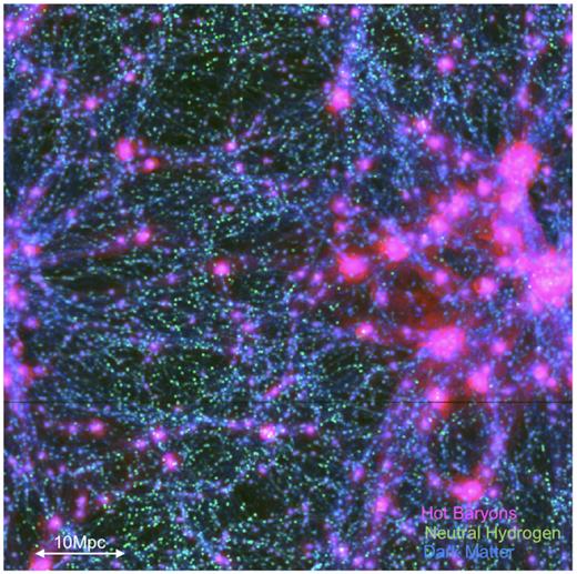
RGB rendering of the matter distribution in our simulated volume for the CSFBH2 model at z = 0.045: DM density (blue), ionized gas (pink), and neutral hydrogen (green).
2.2 Multiwavelength synthetic observations and halo catalogues
We generated emission maps of our simulated volume at different wavelengths, including a number of emission/absorption channels:
- X-ray emission: we assume for simplicity a single temperature and a single (constant) composition for every cell in the simulation, and we compute the emissivity, Λ, from the B-Astrophysical Plasma Emission Code,3 computing continuum and line emission under the assumption of collisional equilibrium, as in Vazza et al. (2019). The metallicity is also assumed to be constant in each cell, Z/Z⊙ = 0.3. For each energy band, we compute the cell’s X-ray emissivity and integrate along the line of sight (LOS):where nH and ne are the number density of hydrogen and electrons (assuming a primordial composition), respectively, T is the gas temperature and dV is the constant volume of our cells.4 In this work, we consider a broad energy range covering the soft X-ray spectrum (from 0.3 to 2.0 keV) as this was shown to yield the highest chances of detection with incoming X-ray telescopes (e.g. Simionescu et al. 2019; Vazza et al. 2019).(1)$$\begin{eqnarray*} S_X(E_1,E_2) [\rm erg\, s^{-1}] = \int {\it n}_H {\it n}_e \Lambda (\it T,Z) \, {\rm d}V, \end{eqnarray*}$$
- Synchrotron radio emission: We compute the emission from relativistic electrons assuming they are accelerated by diffusive shock acceleration (DSA, e.g. Kang, Ryu & Jones 2012, and references therein), accelerating a small fraction of thermal electrons swept by shocks up to relativistic energies (γ ≥ 103–104). We identify shocks in our simulations in post-processing, with a velocity-based approach (Vazza, Brunetti & Gheller 2009), and we compute the radio emission from electrons accelerated in the shock downstream following Hoeft & Brüggen (2007). The radio emission is calculated in post-shock cells as the convolution of the several power-law distributions of electrons that overlap in the downstream cooling region, to which we assign an integrated radio spectrum:where S is the shock surface, |$\xi _e(\mathcal {M})$| is the acceleration efficiency of electrons as a function of Mach number (see Vazza et al. 2017, for details), ν is the observing frequency, B is the magnetic field strength in the post-shock cell and BCMB is the magnetic field-equivalent to the CMB energy density (|$B_{\rm CMB}=3.2 \rm \,\mu G (1+z)^2$|). Our model does not account for radio galaxies, which are an important contributor to the radio emission from the cosmic web. However, our masking procedure (see Section 3.1) makes the presence of radiogalaxies in the simulation irrelevant, as the cross-correlations in such case are computed after removing their putative location from the sky model. Moreover, we do not include the contribution from the additional diffuse radio emission which may be produced by secondary electrons (Dolag & Enßlin 2000) and/or turbulent re-acceleration (Brunetti et al. 2009). Both these scenarios have been proposed for the origin of ‘radio haloes’ (e.g. see Brunetti & Jones 2014; van Weeren et al. 2019, for recent reviews), but their contribution should be largely sub-dominant compared to the radio emission from cosmic shocks starting from the periphery of haloes (e.g. Vazza et al. 2015).(2)$$\begin{eqnarray*} P(\nu) \rm \left[\frac{erg}{s \cdot Hz}\right]=6.4 \times 10^{34} \int \frac{\it S \,n_{\rm e} \xi _{\rm e}(\mathcal {M}) \,T^{\rm 3/2}}{\nu ^{s/2}} \cdot \frac{{\it B}^{1+s/2}}{{\it B}_{\rm CMB}^2+{\it B}^2} d{\it V}, \nonumber\\ \end{eqnarray*}$$
- Faraday Rotation (RM): we define for each beam of cells along the LOS in each map the Faraday Rotation experienced by linearly polarized radio emission aswhere |$\rm ||$| denotes the component of the magnetic field parallel to the LOS, z is the redshift of each cell, ne is the physical electron density of cells, assuming a primordial chemical composition (μ = 0.59) of gas matter everywhere in the volume (e.g. Vazza et al. 2017).(3)$$\begin{eqnarray*} \rm RM \ \rm [rad\, m^{-2}]=812 \int \frac{{\it B}_{\rm ||}}{\rm [\mu G]} \cdot \frac{{\it n}_e}{\rm [cm^3]} \frac{\it dl}{[kpc]}\frac{1}{1+{\it z}}, \end{eqnarray*}$$
- SZ effect: we compute the SZ signal at 21 cm of the specific intensity of the CMB at the frequency ν, assuming a small optical depth everywhere, aswhere TCMB is the CMB temperature, which is appropriate for the Rayleigh-jeans part of the CMB spectrum (e.g. Birkinshaw 1999), σT is the Thomson cross-section, kb is the Boltzmann constant, me is the electron mass, and c is the speed of light.(4)$$\begin{eqnarray*} \Delta I_{\rm SZ}(\nu) [\rm Jysr^{-2}] = \frac{4 {\it k}_{\rm b}^2 \sigma _T {\it T}_{\rm CMB} }{{\it m}_e c^2} \left(\frac{\nu }{\it c} \right)^2 \int \rm \frac{\it dl}{\rm [cm]}\, \frac{{\it n}_e}{\rm [cm^3]} \frac{\it T}{[K]}, \end{eqnarray*}$$
- Neutral Hydrogen radio emission: we estimate the spin temperature of H i and its related signal following Horii et al. (2017). In summary, the spin temperature is computed assuming three physical processes: (a) the excitation and de-excitation by the CMB photons; (b) collisions with electrons and other atoms; and (c) interactions with background Lyman-α photons (Field 1959):where xc and xα are the coupling coefficients for the collisional process and the interaction with Lyα photons, while Tα is the colour temperature in the vicinity of the Lyα frequency. Formulas for xc, xα, and Tα and for the Lyman-α background mean intensity Jα, are given in Horii et al. (2017).(5)$$\begin{eqnarray*} T_{\rm HI}\rm [K]=\frac{1+{\it x}_{\rm c}+x_{\alpha }}{{\it T}_{\rm {CMB}}^{-1}+{\it x}_{\rm c}{\it T}^{-1}+{\it x}_{\alpha } {\it T}_{\alpha } ^{-1}} , \end{eqnarray*}$$
While in CSFBH2 model the H i abundance is computed in a self-consistent way by enzo chemistry modules, in the non-radiative runs we simply assume a fixed reference value of 10−6 for the fraction of the gas density, value that is commonly found in simulations (e.g. Popping et al. 2009) at gas temperatures |$T \le 10^{5}{-}10^{6} \, \rm K$|. In principle, the contribution from H i can be computed even in a simple non-radiative simulation, assuming that the thermal and ionization evolution of gas in filaments is fully determined by the combined effect of the background UV radiation and of the Hubble expansion (e.g. Villaescusa-Navarro et al. 2018). However, the shock heating by large-scale shocks and, possibly, the feedback from active galaxies, both included in our simulations, are expected to affect the properties of filaments in H i. Neglecting these effects leads to underestimating the temperature in filaments and this grossly overestimates the neutral hydrogen fraction. Therefore, only our CSFBH2 model includes the necessary physics to provide a robust estimate of the H i temperature, while the other two runs are only presented for completeness, but are not realistic enough.
Galaxy and galaxy clusters/groups have been extracted as DM haloes from the simulated data using the following procedure. First, we identify the local maxima in the DM mass density field above a given threshold, which is set according to the typical number of objects expected from a given observation. For instance, setting the threshold |$\rho _{th} = 2 \times 10^{-30}\, \rm g\, cm^{-3}$|, our procedure identifies |$N_{\rm g} \approx 220\, 000$| haloes in the 853|$\rm Mpc^3$| volume, corresponding to a density of ∼0.35 galaxy per comoving |$\rm Mpc^3$| and a projected galaxy density of ∼3520 galaxies per square degree, consistent with the expected number count of galaxies at low redshift by Euclid, which is ∼3 × 10³–104 galaxies per square degree (e.g. Boldrin et al. 2012). A halo is then reconstructed around each peak, with a spherical overdensity algorithm which computes the radial mass profile of haloes within concentric shells. Increasingly larger spheres are built around the peak until the internal average mass overdensity is equal to N. The corresponding radius, RN, defines the size of the halo. In our case, we have produced the halo catalogues for R100 and R200. The case R500 has also been calculated, being more in line with real X-ray observations at the scale of groups of galaxies (Eckmiller, Hudson & Reiprich 2011; Reichert et al. 2011) discussed in Section 2.3. Small objects, typically with masses |$M_{\rm 100} \le 10^{10} \, \rm M_{\odot }$|, can have a diameter close to the resolution of the simulation. In that case, we assign to the galaxy the radius corresponding to a single computational cell.
An RGB rendering of the projected X-ray emission, radio emission, and H i emission in our CSFBH2 model at z = 0.045 is shown in Fig. 2, well illustrating once more how the different emission proxies considered in this work have a different level of clustering with the underlying large-scale distribution of the cosmic web.
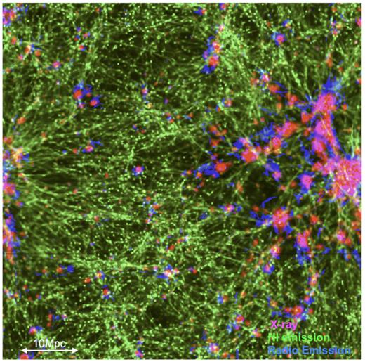
RGB rendering of the distribution of different observable quantities for the same volume and model of Fig. 1: synchrotron radio emission (blue), H i emission (green), and X-ray emission (pink).
For the sake of simplicity, we neglect in all cases the contribution from the Galactic foreground, as well as the intrinsic contribution from galaxies (e.g. internal Faraday Rotation or X-ray/radio emission from active galactic nuclei) as they cannot be properly resolved in our cosmological simulations.
As a reference, our simulated volume has been located at z ≈ 0.045 (dL ≈ 200 Mpc). Images consist of 1024 × 1024 pixels, meaning that each simulated sky model has a pixel resolution of |$\approx \!90\,{\rm arcsec}\, \mathrm{pixel}^{-1}$| for the assumed cosmology.
2.3 Validation of models
As a preliminary step, we have validated the models adopted in this work in order to assess their reliability for the objectives of our study. Additional tests (for the larger set of the Chronos++suite of simulations) can be found in Vazza et al. (2017).
The mass–temperature scaling relations of groups and clusters of galaxies in our simulations are presented in Fig. 3. The clusters/groups are identified as spherical haloes at R500 (see Section 2.2). The results are similar to what already discussed in Vazza et al. (2017) for the larger set of simulations of our Chronos++suite: while the non-radiative runs (baseline and DYN5) strictly follow, as expected, the self-similar T ∝ M2/3 relation, the combined effects of radiative cooling, star formation, and feedback from black holes in the CSFBH2 run steepens the scaling relation within R500, more in line with real X-ray observations at the scale of groups of galaxies (Eckmiller et al. 2011; Reichert et al. 2011). This is an effect of the increased temperature within R500 of |$M_{\rm 500} \le 10^{14}\, \mathrm{M}_{\odot }$| systems, in which the total feedback energy is of the same order of the gas potential energy. This ensures that, in general, the large-scale distribution of thermal gas in our simulations is realistic enough compared to the expected properties of galaxy clusters. In addition, the introduction of AGN feedback in run CSFBH2 modifies our lowest mass systems in a way compatible with observational data, for realistic feedback parameters.

Fig. 4 shows the cosmic SFR history for run CSFBH2, compared to the survey of infrared and ultraviolet observations from Madau & Dickinson (2014). The match is reasonably good at all epochs/redshift, indicating that overall our ad hoc prescription for star formation and feedback performs well in converting the gas cooling within haloes into star-forming particles, as well as that the amount and duty cycle of feedback in our haloes is fairly compatible with observations (see Vazza et al. 2017 for more details).
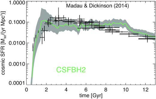
Simulated cosmic star formation history for our CSFBH2 run (coloured lines with ±3σ variance) against the observed cosmic star formation history from the collection of observations in Madau & Dickinson (2014) (black points with error bars).
In Fig. 5, we show the distribution of H i column density for three different epochs (z = 0.0, 0.5, and 1.0) in the CSFBH2 model, compared to observations (e.g. Corbelli & Bandiera 2002; Shull et al. 2017). At all epochs, the agreement is far from being satisfactory, with a lack of H i absorbers both for |$N_{\rm H} \le 5 \times 10^{15} \rm \,cm^2$| and |$5 \times 10^{18} \rm \,cm^2$|. This suggests that the emergence of neutral hydrogen in our model is undermined by the insufficient spatial resolution, which is a key factor for the formation of H i in the circumgalactic medium, as well as at low column densities (e.g. Hummels et al. 2018). This is a caveat to be considered in interpreting our results in the remainder of the paper.
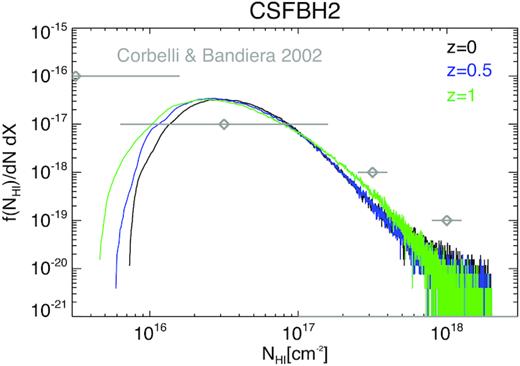
Differential distribution of H i column density at three epochs in our CSFBH2 run. The additional grey points with error bars are derived from Corbelli & Bandiera (2002).
Fig. 6 gives the scaling between the integrated synchrotron emission at 1.4 GHz and the X-ray luminosity in the (0.1–2.4 keV) band of host clusters within, in this case within R200 (i.e. 200 time the critical cosmic matter density) to compare with the observed statistics of ‘radio relics’ in galaxy clusters (e.g. Nuza et al. 2017), which are believed to represent the tip of the iceberg of the distribution of radio emission in the cosmic web. Despite the lack of massive haloes, due to the limited volume simulated here, we can compare with observations by extrapolating to lower masses/X-ray luminosity the (P1.4, LX) scaling found by de Gasperin et al. (2014), as shown in the figure. Albeit with a large scatter, the relic radio emission from our population of clusters is reasonably consistent with the observed distribution of radio relics, which, in turn, suggests that the synchrotron model adopted here (see equation 2) is plausible for all models as it does not violate available radio constraints.
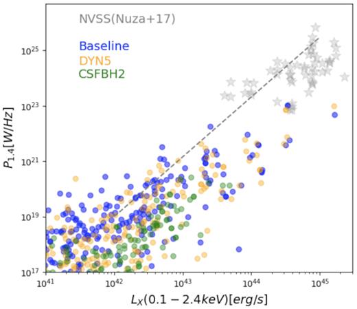
Simulated versus observed scaling relation between the X-ray luminosity in the (0.1-2.4) keV band and the total radio power at 1.4 GHz from radio relics. The observational data (stars) are taken from Nuza et al. (2017), while the black-dashed line is derived from the best-fitting relation by de Gasperin et al. (2014).
Despite the aforementioned difficulty in resolving galaxy formation physics with our runs (Section 2.1) and in properly identifying small objects (Section 2.2), the statistical large-scale clustering properties of the haloes within filaments are well resolved and described by our approach, as shown by Fig. 7, that presents their two-points correlation function. For all models, the function resulted to follow a power law with exponent γ = −1.899 ± 0.0657 for the baseline model, γ = −1.867 ± 0.067 for DYN5, and γ = −1.828 ± 0.071 for the CSFBH2 model, in the range 0.1 to 10 Mpc, consistent, although slightly steeper (given the reduced small-scale power due to the limited resolution) with that expected for galaxies in the standard ΛCDM model (Weinberg et al. 2004). This was shown also in Gheller et al. (2016), where the same procedure was adopted to compare the resulting halo catalogues with the GAMA data (e.g. Alpaslan et al. 2014). The normalization (in arbitrary units) of the various correlation functions differs only slightly. The similarity of the different curves points out how the clustering properties of the haloes are only mildly influenced by the different physical setup characterizing the various simulations.
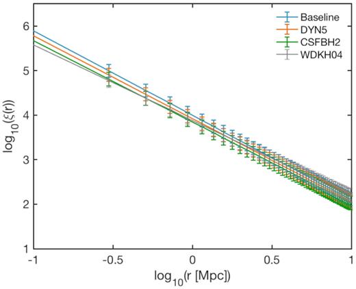
The two-points correlation function in the range 0.1–10 Mpc, in arbitrary units, of the haloes extracted from the three runs (coloured lines), compared with that from Weinberg et al. (2004) (grey line). 3σ error bars are shown.
In summary, the physical models used in this work are realistic enough to present a first systematic study of the cross-correlation between different observable signatures of diffuse gas and magnetic fields in the cosmic web.
3 CROSS-CORRELATION
In the case of our maps, the significance of the cross-correlation is evaluated against the case of null correlation, for which Cr is computed between A and B from two different projections. As an example, Fig. 8 shows the autocorrelation function of the DM mass density distribution for the three models, calculated cross-correlating each image with itself, compared to the same quantity but calculated correlating each image with one of the remaining two projections. Such comparison gives an indication of the shape of the signal expected from perfectly correlated images, equal to one at zero displacement and then monotonically decreasing with increasing shifts, compared to that of perfectly uncorrelated ones, which is randomly fluctuating around zero at all displacements.
Autocorrelation function of the DM mass density distribution for the three models. Solid lines are calculated cross-correlating each image with itself and averaging over the three orthogonal projections. Dashed lines represent the null reference baselines, calculated cross-correlating each image with one of the remaining two projections and averaging the the results.
3.1 Masking of haloes
In order to separate correlation signals due to gas within haloes and outside them, we calculate the cross-correlation both on full maps, and on ‘masked’ ones, excising the information coming from the haloes, and focusing on the contribution from the cosmic web only. Masking allows also to exclude those regions where the limited resolution of our models may have a major impact on the simulated formation of galaxies and on their impact on our observables.
Masking is performed projecting the halo catalogues on the maps and setting to −1 all the pixels within circles centred on each halo centre and radius RN. In calculating the cross-correlation, all pixels with value −1 can then just be discarded. We have tested two different masks, corresponding to the catalogues R100 and R200, respectively (see Section 2.2). We anticipate that the results obtained adopting the two different masking radii do not show meaningful differences in all cases, therefore in the rest of the paper, we discuss the R100 case only. Examples of the R100 masked maps are shown in Fig. 9.
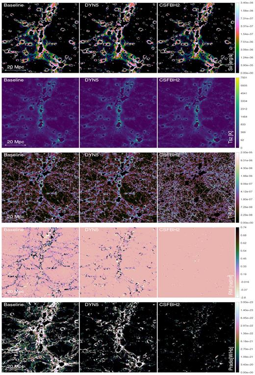
Example of projected maps of various observables: from the top to bottom: X-ray emission in the (0.3-2) keV band, Sunyaev–Zeldovich signal computed at |$200 \, \rm GHz\,$|, H i brightness temperature at 1.4 GHz, Faraday Rotation measure and synchrotron radio emission at 200 MHz, for our three models and for a |$85^3 \rm \,Mpc^3$| volume located at z = 0.045. R100 masking is applied.
4 RESULTS
In this section, we present the results obtained calculating the cross-correlation between the quantities introduced in Section 2.2, for the different models.
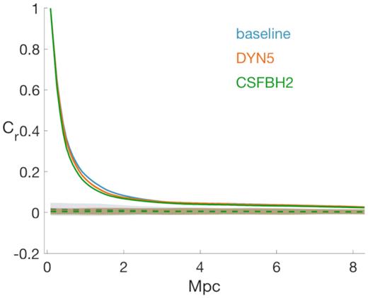
Fig. 10 shows the cross-correlation between the halo maps and the DM mass density, showing the expected correspondence between haloes and mass distributions. The baseline and the DYN5 models are indistinguishable, magnetic fields having no meaningful impact on the DM dynamics. For the CSFBH2 model, the correlation drops faster than for the other two models with separation. In this case, in fact, cooling and energy feedback affects the gas dynamics, with non-negligible feedback on the overall mass distribution. The loss of correlation above 0.5 Mpc is due to the formation of more compact collapsed objects, due to the cooling, combined with the effect of AGN outflows, wiping out overdensities in affected regions.
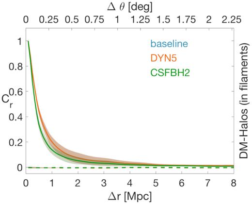
Cross-correlation between the DM mass and the halo distributions. Halos are identified as local maxima of the DM density field. In the base horizontal axis, the scale is in Mpc, in the upper horizontal axis the scale is in degrees.
4.1 Cross-correlation analysis of physical models
We first study the cross-correlation of different quantities, without the inclusion of any observational noise or instrumental effect, focusing on the impact of the model variations of our set of simulations.
4.1.1 Cross-correlation with the DM distribution
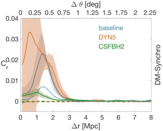
Fig. 11 gives an overview of the cross-correlation of the five observables, synchrotron emission, RM, H i temperature, SZ effect, and X-ray luminosity with the DM mass distribution. The left-hand panel gives the cross-correlation between unmasked maps, while the right-hand panel shows the R100 masking case (all regions containing haloes or clusters are masked out from the calculation, see Section 3.1). The correlation curves and their variance, are calculated averaging along the three orthogonal projections, considered as independent.
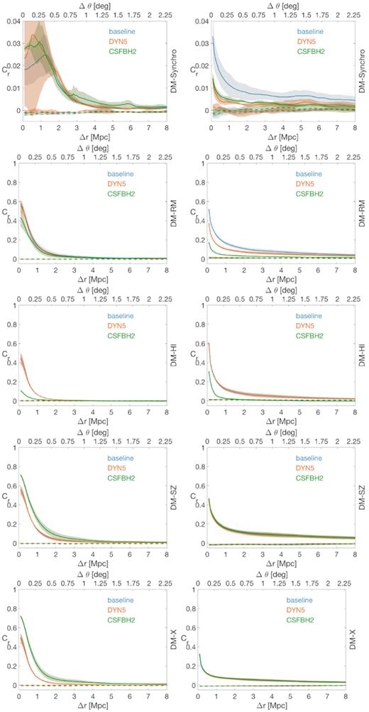
Cross-correlation of the DM mass distribution and the synchrotron emission (first row), the rotation measurement (second row), the H i temperature (third row), the SZ effect (fourth row) and the X-ray luminosity (bottom row). The cross-correlation is normalized to the corresponding null model. The first column takes into account the unmasked images, while in the second column galaxy clusters and haloes have been masked at R100. The coloured shaded bands represent the 1σ statistical uncertainty in the calculation of the cross-correlation, while horizontal dashed lines give the reference correlation of the null model with its 1σ statistical uncertainty. In the base horizontal axis, the scale is in Mpc, in the upper horizontal axis the scale is in degrees.
All cross-correlations show a significant signal at least out to |$\sim 1 \,\rm Mpc$|, which corresponds to an angular scale of θ ∼ 17 arcmin at z ≈ 0.045. The cross-correlation between the DM and the synchrotron radiation presents the most peculiar features. The unmasked data show that, differently from all the other correlations, DM and radio emission have a maximum correlation not at displacement 0, where the mass density peaks, but at a distance between 1 and 2 Mpc. There, strong accretion shocks develop, compressing the gas, which increases the intensity of the magnetic field, and accelerating cosmic rays, leading to an overall enhancement of the radio signal. When masking is applied, the highest density regions, in which the behaviour of mass and radio emission depart from each other, are removed from the statistics and the cross-correlation tends to follow a monotonically decreasing (with increasing distance) trend. Although the signals are well above the null model, their absolute values are one order of magnitude lower than those found for the other quantities. This is understood because, unlike all other observable, the radio emission is in our model is not a continuous function of the gas density field, but gets ‘lighted on’ only in shocked cells, hence not all pixels in our sky model contain synchrotron emission, introducing gaps in our radio maps. This also leads to the estimated large variance, which can be interpreted as a projection effect, strong radio emissions spots randomly falling on the same line of sight as the mass density peak. The variance, in fact, is much lower for the masked data, in which the highest density peaks have been removed.
It is interesting to notice that, in the case of unmasked data, the strongest correlations are found for the DYN5 and the CSFBH2 models, while the baseline model shows the weakest signal. By construction, the average magnetic field strength in the central regions of our haloes is similar in all models, but runs with dynamo amplification or injection by AGN produce a larger spread of the magnetic field magnitude, which is amplified in the synchrotron signal (which approximately scales as ∝ B2). Therefore, in these two models, the cross-correlation between radio emission and the DM distribution is slightly boosted at a small separation, considering that most of the signal is originated by haloes and by the merger shocks they contain. The trend gets similar at large distances in all models, albeit with slightly higher signal in the CSFBH2 model, due to the presence of extra magnetic fields and shock waves from satellite haloes (and the AGN they contain). The opposite trend is found for the masked results, i.e. in the baseline model, the cross-correlation signal is higher, because in this case similar large-scale accretion shocks are present in all models, and the average magnetic field strength remains higher in the baseline one (due to the much higher primordial value), while it sharply drops in the other two scenarios.
For similar reasons, a significant cross-correlation between the RM and the projected DM distribution is present out to a scale of |$\sim 2 \rm \,Mpc$| in the baseline model, even with the R100 masking (and likewise for the radio emission). Conversely, the correlation drops below significance at approximately half of this scale for the DYN5 model, and even at shorter distances for the CSFBH2 model.
All the cross-correlations of the remaining quantities with the DM decrease with increasing displacement. The cross-correlations involving the hot gas distribution (X-ray and SZ) are rather similar. The baseline and DYN5 models have lower correlations compared to the astrophysical model, but this difference tends to disappear in masked maps. Even when haloes are masked out, the cross-correlation signal is significant at the ≥1σ level out to |$\sim 1 \rm \,Mpc$| both in X-ray and SZ. On the other hand, in the unmasked analysis, we systematically measure a higher signal for |$\le 2{-}3 \rm \,Mpc$| in the CSFBH2 model, which is understood because in radiative simulations haloes tend to have higher central concentration and correlate slightly more with the DM distribution (e.g. Teyssier et al. 2011). This is in line with the simulated cross-correlation analysis between thermal SZ and gravitational lensing (Battaglia, Hill & Murray 2015), in which the impact of AGN feedback is limited to θ ≤ 10−20 arcmin.
Significant differences between models are found by cross-correlating the H i temperature and the projected DM density distribution, with the non-radiative runs showing the largest correlation at all scales. However, as we noticed in Section 2.2, in such runs our assumed fixed (10−6) neutral hydrogen fraction clearly gives a gross overestimate of the H i abundance in the hottest gas phase of the cosmic web; hence, only the CSFBH2 models are to be considered realistic here, and in this case, a significant excess in the cross-correlation between the projected DM density and the H i temperature decrement is significant only up to |$\sim 1 \rm \,Mpc$|, also with the masking of our sky model up to R100.
In summary, at least in principle, the statistical correlation between the halo/DM distribution and radio observables is a promising tool to probe the amplitude of extragalactic magnetic fields, even outside of the cluster volume usually explored by existing radio observations. This will offer a powerful tool to tell competing models of magnetogenesis apart. On the other hand, observables related to thermal gas are well correlated with the DM/galaxy distribution out to several |$\rm Mpc$|, with little dependence on the underlying AGN activity.
4.1.2 Cross-correlation between other observables
In Fig. 12, we present a selection of the cross-correlations between different gas-related quantities. While they do not show outstanding differences compared to the trends outlined above, we report them for completeness. Furthermore, they provide ‘first-order’ guidelines for possible future attempts of adopting the cross-correlation analysis for instruments different from those considered in this work.
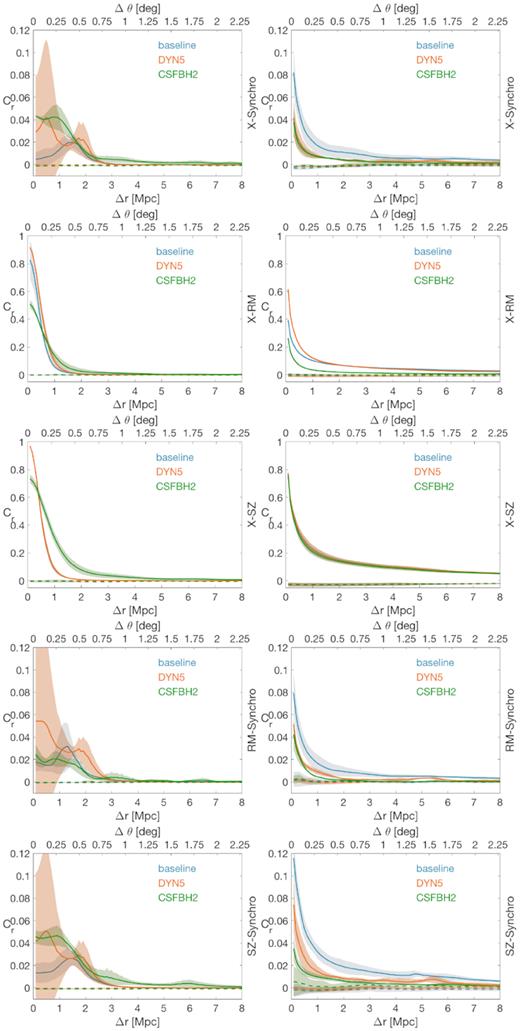
Cross-correlations between gas-related quantities. The first row accounts for the unmasked images, while in the second column galaxy clusters and haloes have been masked at R100. The coloured shaded bands represent the 1σ statistical uncertainty in the calculation of the Cross-correlation, while horizontal dashed lines give the reference correlation of the null model with its 1σ statistical uncertainty. In the base horizontal axis, the scale is in Mpc, in the upper horizontal axis the scale is in degrees.
With the exception of synchrotron emission, all other gas-related quantities strictly follow the total-mass distribution and cross-correlate at small displacements.
The cross-correlations between X-ray and RM or SZ and between RM and SZ have the highest and cleanest signal, hence they appear to be the most promising for detection. On the other hand, the cross-correlations between synchrotron radio emission and SZ, X-ray emission, and RM tend to be weaker in absolute value (owing to the intermittent nature of radio emission in our model, as above) but spatially broader, with the extreme case of baseline model in which a significant cross-correlation with all quantities can be measured out to 4–5 Mpc. In the case of the radio sky model, large statistical errors affect the unmasked data (following the rare occurrence of central merger shocks), while masked data results to be less noisy. The signal is low (always below 0.1), but significantly higher than the null model, especially in the correlations with X and RM.
Finally, all cross-correlations involving H i in the CSFBH2 model (not shown), the only one treating self-consistently the H i component, are very weak, with trends similar to the cross-correlation with DM presented in the previous section. Little correlation is found even at null displacement, which is expected because in the CSFBH2 model (the only one in which a basic chemical evolution model is adopted at run time) H i almost never forms within hot and massive haloes, hence a large SZ and X-ray signal anticorrelates with H i temperature. For unmasked data, the cross-correlation tends to zero at scales between 1 and 2 Mpc, being dominated by the collapsed, high-density structures. Such correlation length tends to be larger for masked data, since random correlations are statistically more frequent considering the filamentary large scale distribution of matter only.
4.2 Cross-correlation analysis including observational effects
In this section, we focus on the most significant selection of cross-correlations between our observables, with observational/instrumental noise added. The purpose is that of assessing which signatures of the cosmic web may be potentially detectable with present-time surveys, in the near or in the more remote future.
In detail, we first consider a representative set of currently available instruments at all wavelengths (e.g. eROSITA,5 ASKAP,6 LOFAR-HBA,7 Meerkat8, and PLANCK9), while for future instruments we assume the performance of a few notable planned/proposed instruments (e.g. ATHENA-WFI,10 SKA-MID and SKA-LOW11, and AtLAST12). Our approach here is to refer to the nominal sensitivity/performance of the various surveys, as presented in their reference papers and/or official websites. In most cases, these sensitivities can be reached in the search of diffuse emission only in the ideal case of a full removal of point-like sources and foreground emissions as well as under the assumption of a perfect calibration of the instruments.
For the projected galaxy distributions, we set the threshold of projected DM density so that it is compatible with the present sensitivity of the WISE IR survey, yielding ∼10 galaxies per square degree for z ≤ 0.07 (Vernstrom et al. 2017), and the future sensitivity by EUCLID, which should give ∼103–104 galaxies per square degree in the same redshift range (e.g. Boldrin et al. 2012).
We should preliminary notice that producing synthetic observations convolved for the specific resolution of each different instrument is out of the scope of the paper. Here, we mostly target emission or absorption features from large scales of the cosmic web. Our pixel resolution (90 arcsec) is thus coarser than what can be achieved by several instruments. One example is the rotation measure of background polarized radio sources, which can get to ∼10 arcsec. However, we do not consider this problematic for our science goal here, as recent papers have shown that the simulated RM only drops by a factor of a few when large beams are applied to convolve the simulated radio signal (Vazza et al. 2018; Wittor et al. 2019). Moreover, previous resolution studies have shown that the three-dimensional (3D) properties of the magnetic field in filaments and/or outside galaxy clusters are overall little affected by resolution (e.g. Vazza et al. 2014). Therefore, our predictions here are reasonably accurate (within a factor of ∼2–3 on RM) in the case of the diffuse intergalactic medium of the cosmic web.
As an exception, in the case of PLANCK SZ observations, the resolution beam is ≈5 arcmin, coarser than our mock sky model. However, our simulations do not show much structure in the SZ from the cosmic web on large scale, hence the cross-correlation analysis we present here is reasonably robust against modest inhomogeneities in the simulated versus real beam size of observations.
Only for the specific comparison with MWA observations, discussed in Section 4.2.1, we tuned the spatial resolution of the mock observation in order to compare more closely with recent observations.
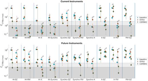
The two panels of Fig. 13 give a synthetic overview of the predicted cross-correlation signal for current and future instruments. We give the values of the amplitude of the cross-correlation at null displacement or at the fixed reference displacement of 1 Mpc, both for the unmasked and for the R100 masked models. For a homogeneous presentation of data, we normalized the cross-correlation signal at these two reference separations by the maximum cross-correlation of the corresponding null model, which now accounts for the contribution of both the cosmic variance and the noise assumed in each specific observation.
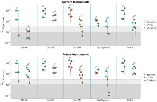
Cross-correlation of DM with H i temperature (first block – each block is the area delimited by vertical blue lines), SZ (second block), rotation measurement (third block), synchrotron emission (fourth block), and X-ray luminosity (fifth block), in presence of noise due to different instruments. The top panel shows the results for ‘current’ instruments and the bottom panel for ‘future’ instruments (see Table 2 for details). Within each block, each group of three represents a different masking. Within each group of three: To the left-hand side is the baseline model (blue circles), at the centre is the DYN5 model (orange squares) and to the right-hand side is the CSFBH2 model (green diamonds). The top symbol is the maximum correlation, and the bottom symbol is the correlation at 1 Mpc displacement (≈17 arcmin separation). Horizontal grey stripes show the null model 1σ and 3σ uncertainty. Error bars represent the standard deviation of the cross-correlation function calculated over the three orthogonal projections.
Several interesting trends can be noticed:
DM–HI correlation: The cross-correlation between IGM and DM in the most realistic model (CSFBH2) becomes nearly impossible to be detected by present instruments (e.g. Meerkat/ASKAP), while it should be detectable up to R100 using the SKA-MID (mostly in Phase II), in agreement with Horii et al. (2017). The amplitude of the signal falls rapidly when the clumpiest portion of the sky model is excised. However, the impact of our limited spatial resolution in modelling the formation of H i even outside of haloes is yet to be assessed with higher resolution simulations.
DM–SZ correlation: The cross-correlation holds up to ∼1 |$\rm Mpc$| even when haloes are masked out, with little dependence on the assumed physical model, with both current and future instruments.
DM–RM correlation: For an |$\sim \, \rm rad\, m^{-2}$| sensitivity level, the significant detection of cross-correlation seems possible even when haloes are masked out, for a significant scale magnetic field as in our baseline model. The detection at R100 becomes marginal for the sub-grid dynamo model, and impossible in the CSFBH2 scenario. However, a ten-fold increase in RM sensitivity, as expected to be possible with the SKA-MID in Phase II, may allow detecting RM outside of haloes even in the CSFBH2 model, and hence discriminate between magnetogenesis scenario using RM grids.
DM–synchrotron correlation: Similar to the previous case, but with somewhat lower significance, detections are possible outside of haloes in the primordial case, with a sensitivity of the order of |$\sim \, \rm \mu Jy\, arcsec^{-2}$| as in LOFAR-HBA. Detection will be even more clear with the SKA-LOW in this scenario. Also in the dynamo amplification model future, SKA-LOW observations should allow to marginally detected a positive cross-correlation with the underlying galaxy distribution. Detecting the signature of radio emission outside of haloes in the CSFBH2 model will remain challenging even with SKA-LOW, due to the rapid drop (Pradio ∝ B2 for |$B\ll 3.2 \rm \,\mu G$|) of the radio emission away from haloes (Vazza et al. 2017), in the case magnetic fields are only seeded by processes linked to galaxy formation.
DM–X-emission correlation: When the correlation at 1 Mpc is concerned the robust detection of the correlated signal from X-ray emission in the soft band appears fully feasible only with future instruments, i.e. with ∼100 ks integration with Athena-WFI (in line with Vazza et al. 2019). Statistical detections using present instruments, like eRosita, are extremely challenging, with little dependence on the assumed gas physics. Thus for a proper imaging of the WHIM in the cosmic web, a new concept of X-ray telescope must be deployed, for which proposals have been submitted (e.g. The Lynx Team 2018; Simionescu et al. 2019).
In summary, with presently available surveys of galaxies and with current multiwavelength instruments, the best chances of detecting the correlated signal of the diffuse IGM outside of haloes and in filaments come from SZ observations (regardless of adopted gas physics, e.g. Fabjan et al. 2010; Battaglia et al. 2015).
Additional chances of detecting the magnetized cosmic web in correlation with the galaxy distribution may come from surveys of Rotation Measure, in case of the significant volume-filling magnetic fields (|$\ge 1\!-\!10 \rm \,nG$|) expected from a primordial scenario as in our baseline model. Conversely, a robust non-detection of such correlated signal with surveys of RMs can already restrict the allowed amplitude of primordial magnetic fields, at the |$\le \rm \,nG$| level.
However, in practice, the effective sensitivity of any RM survey can be limited due to the contribution from the foreground Faraday screen by our galaxy as well as by the intrinsic RM from polarized background sources, both challenging to remove (see discussion in Locatelli, Vazza & Domínguez-Fernández 2018). By studying the dependence with the redshift of RM from a quasar sample, Han (2017) concluded that ∼104–105 measured RMs may be necessary to tell apart Galactic from extragalactic contribution in such objects. The ever-growing knowledge of the 3D structure of the Galactic magnetic field should also improve alongside the growth of RM samples, enabling the removal of the Galactic foreground, in combination with other observables (such as extragalactic RMs, PLANCK polarization data, galactic synchrotron emission and observed distribution of ultrahigh-energy cosmic rays, see Boulanger et al. 2018 for a recent review). Therefore, the theoretical RM sensitivity that should be reached by the SKA-MID (∼0.1 |$\rm rad\, m^{-2}$|) is a very optimistic one, which can only be achieved in presence of major advances in the modelling of the polarization sky.
On the other hand, the somewhat reduced significance of the correlation between DM and synchrotron emission in most models should be balanced by the fact that it is comparatively easier to remove the foreground contribution to the radio sky (e.g. based on the spectral index of the observed emission), and that the emission from radio galaxies is generally well confined in host clusters/groups, and is hence enclosed within the masked areas. Therefore, the challenging statistical detection of the cosmic web in total radio intensity may offer a strong case for the study of cosmic magnetism.
Finally, we considered mixed cross-correlation between observables that directly trace the gas component and/or the magnetic fields, with the same realistic sensitivities considered above, as shown in Fig. 14. The most promising cross-correlation appears to be between the SZ effect and the synchrotron emission, at least in the primordial scenario. Marginally detectable cross-correlations are present between the SZ effect and RM, especially for the primordial and for the small-scale dynamo amplification case.
Cross-correlation of various gas-related quantities among each other. H i temperature with SZ (first block – each block is the area delimited by vertical blue lines), RM (second block), X-ray luminosity (third block) and synchrotron emission (fourth block), synchrotron emission with SZ (fifth block), RM (sixth block) and X-ray luminosity (seventh block), X-ray luminosity with SZ (eighth block) and RM (ninth block), RM and SZ (last block) in presence of noise due to different instruments. The top panel shows the results for ‘current’ instruments and the bottom panel for ‘future’ instruments (see Table 2 for details). Symbols and grouping follow the same rules as in Fig. 13.
In more futuristic scenarios many of such correlation may become detectable, even at the distance of 1 Mpc and adopting masking. The correlation between SZ effect and synchrotron emission should be prominently detectable in the primordial case, and still marginally detectable in the small-scale dynamo amplification scenario, hence offering a way to measure magentogenesis based on the amplitude of detected (or undetected) cross-correlation. Likewise, also significant cross-correlations between SZ effect and RM should be detectable for these two scenarios, as well as between X-ray emission and SZ effect. In all cases, the detection of the cosmic web through magnetic related effects depends on the high sensitivity that should be achieved thanks to the full deployment of the SKA, both in its LOW and MID parts. Interestingly, also cross-correlations entirely produced in the radio domain should detect the cosmic web, i.e. through the synchrotron emission–RM correlation, which would be prominent both in the primordial and in the dynamo model, while it should remain undetectable even by the SKA in case of a purely astrophysical origin of magnetic fields.
4.2.1 Comparison with MWA Phase I cross-correlation
Finally, we attempt a qualitative comparison with the recent results by Vernstrom et al. (2017), who have cross-correlated the radio emission in MWA Phase I observations and the galaxy distribution from the WISE + 2MASS galaxy survey, for a 22 × 22 deg2 field of view. This work reported no statistically significant detection of cross-correlation on ≥ 20 arcmin scales, while the correlated signal on smaller angular scales is likely due to the contamination of unresolved radiogalaxies within the resolution beam of MWA.
Here, we assumed the same sensitivity and resolution beam quoted by Vernstrom et al. (2017) for MWA Phase I observations at 180 MHz, as well as lowered the number of detected galaxies in order to mimic the WISE and 2MASS statistics. In detail, we convolved our radio sky model using a θ ≈ 2.9 arcmin resolution beam (e.g. ∼2 times larger than what we used in the rest of the paper) and considered a noise level of |$0.96 \rm \,mJy\, beam^{-1} \approx 0.028 \rm \,\mu Jy\, arcsec^{-2}$| at 180 MHz, corresponding to the deepest MWA (Phase I) observations used in Vernstrom et al. (2017). To match the galaxy density used in Vernstrom et al. (2017), we used a DM density threshold higher than in the rest of the paper: |$\rho _{th} = \sim 6 \cdot 10^{-29} \rm \,g\, cm^{-3}$|. No masking of haloes is used in this case.
Our results are shown in Fig. 15, and shall be compared with Vernstrom et al. (2017) results for their lowest redshift sub selection of data (z ≤ 0.13). We cannot readily compare with the cross-correlation values given by Vernstrom et al. (2017) in a quantitative way, owing to the different approaches in estimating the noise level of the cross-correlations. Therefore, our synthetic observation can only qualitatively address which model seems to be more compatible with MWA observations.
Cross-correlation between the DM mass and the synchrotron emission adopting the MWA set-up. Lines and bands have the same meaning as in Fig. 11. Blue dotted–dashed line represents the baseline model rescaled down 100 times.
The dynamo model gives the largest correlation with the galaxy distribution, followed by the baseline model, while the astrophysical scenarios give the lowest level of cross-correlation. While all models give a significant cross-correlation out to ∼40–5 arcmin, the amplitude of correlation in the primordial and in the dynamo models seem to be too large to have been missing missed by MWA observations. This potentially suggests that a |$1 \rm \,nG$| initial field (resulting into a typical magnetization of filaments of 10–100 nG, as shown in Gheller & Vazza 2019) is too large to be compatible with the lack of detection reported by Vernstrom et al. (2017). If the radio emission is instead rigidly rescaled by a factor 100 downwards, corresponding to an initial magnetic field in the simulation of ≈0.1 nG comoving, the significance of the cross-correlation approaches the one of the astrophysical cases, showing only a weak correlation excess out to ∼20 arcmin. This test also suggests that the efficient amplification of magnetic fields in our dynamo model, introduced ad hoc to mimic the scenario proposed by Ryu et al. (2008) and challenging to directly observe in numerical simulations, is probably not at work in the bulk of filaments in the cosmic web.
As a caveat, we must notice that, given the finite mass resolution of our simulations, we cannot properly form dwarf galaxies in voids (or in a very poor environment, in general). Therefore, even if the number of galaxies is calibrated to be at the level of the galaxy distribution observed in WISE/MASS surveys, our spatial distribution is typically more clustered than in observations. In principle, this can decrease the cross-correlated signal coming from low-density regions in our sample. With future work, we will employ more resolved simulations in order to better address this issue.
5 CONCLUSIONS
In this work, we have used recent MHD cosmological simulations to investigate the use of cross-correlation analysis between different observables of the cosmic web (i.e. X-ray emission, Sunyaev–Zeldovich signal at 21 cm, H i temperature decrements, diffuse synchrotron emission, and Faraday Rotation). Our analysis aims at both interpreting already available observational attempts in this direction (e.g. Vernstrom et al. 2017), and exploring what can be achieved with future multiwavelength surveys.
For the sake of performing an homogeneous study of many observables with the same data set, our analysis is bound to oversimplify several aspects, which we shortly discuss here. The most important limitations of our simulations are related to the effect of the limited spatial resolution on small, high-density peaks in the gas distribution (i.e. small galaxies or galaxy cluster cores).
First, our (fixed) spatial/mass resolution only allows us to treat galaxy formation processes (i.e. star formation, feedback from active galactic nuclei) with the use of sub-grid modelling. While the impact of galaxy formation on to the large-scale dynamics of cosmic plasma have been calibrated and tested in previous works (e.g. Vazza et al. 2017; Gheller & Vazza 2019), the role of galaxy evolution in shaping our observables (most noticeably the formation of neutral Hydrogen in this case) shall be further explored in the future with higher resolution simulations. However, the fact that our analysis considered also masked maps (Section 3.1) allows us to bracket the uncertainties related the densest part of the distribution of cosmic baryons, and by-pass the intrinsic limitations of missing galaxy formation physics.
Our adopted fixed resolution also limits the development of a small-scale magnetic dynamo, which is instead predicted by a few works (Ryu et al. 2008). While previous dedicated resolution tests have found no indications for an increased magnetization of filaments going to even higher resolution, and have proposed physical reasons for the lack of dynamo amplification in cosmic filaments (Vazza et al. 2014; Gheller et al. 2016), our sub-grid dynamo model (DYN5) is explicitly designed to consider the impact of unresolved dynamo amplification in our final magnetic field model. Limited to the comparison with the recent results of Vernstrom et al. (2017), the DYN5 model seems to produce a too large average magnetization of filaments in the cosmic web to be a viable model.
Third, our synthetic observations contain gross oversimplifications concerning the generation of noise in real observations, which has subtleties and different features at different wavelengths. For example, the role of the Galactic Foreground in synchrotron emission and Faraday Rotation is here neglected, as well as the contamination from (pointlike or extended) radio galaxies. On the other hand, the role of the particle and instrumental background on X-ray emission is also treated in an approximate way, by incorporating their effects into our definition of detection threshold.
Finally, we did not produce proper light cones for the various observables (e.g. by stacking several simulated boxes along the line of sight up to a large redshift), but, for the sake of simplicity, we limited our first analysis to a local volume at low redshift.
Given the above limitations, our results suggest that the statistical correlation between the galaxy network and radio observables is a promising tool to probe the amplitude of extragalactic magnetic fields, well outside of the cluster volume usually explored by existing radio observations, allowing to discriminate between competing models of magnetogenesis.
Observable proxies related to the thermal properties of the gas are also well correlated with the galaxy distribution out to several |$\rm Mpc$|, with relatively little dependence on the assumed baryonic physics. We conclude that with presently available surveys of galaxies and with current multiwavelength instruments, the best chances to detect the diffuse IGM outside of haloes via cross-correlation are given by SZ observations.
An additional interesting probe is represented by the correlation between the galaxy distribution and surveys of rotation measure and synchrotron emission. The cross-correlated signal appears to be detectable already with current facilities if the magnetic field in filaments is volume filling and of the order of |$\ge 1\!-\!10 \rm \,nG$|, as expected in our primordial or in the dynamo scenario. However, our first test to mimic the cross-correlation between the WISE/2MASS survey and MWA Phase I observation as in Vernstrom et al. (2017) suggest that |$\le 10 \,\rm nG$| magnetic fields are required in filaments not to violate observational constraints. This can be accomplished in a primordial magnetogenesis scenario with a primordial magnetic fields of strength |$\le 0.1 \rm \,nG$|, or by an astrophysical origin of extragalactic magnetic fields, which would produce little volume-filling magnetic fields in the cosmic web.
With future work, we plan to improve on some of the limitations outlined above, i.e. by modelling longer light cones and including more realistic templates of noise in synthetic observations, which can be crucial in order to quantitatively assess the robustness of possible (albeit marginally significant) detections of diffuse emission from the cosmic web in existing and future cross-correlation studies. In the meantime, the main results of our current cross-correlation analysis, for different models and observables, are publicly available at https://cosmosimfrazza.myfreesites.net/library-of-cosmic-web-properties.
SUPPORTING INFORMATION
Figure S1
Figure S2
Figure S3
Figure S4
Please note: Oxford University Press is not responsible for the content or functionality of any supporting materials supplied by the authors. Any queries (other than missing material) should be directed to the corresponding author for the article.
ACKNOWLEDGEMENTS
The cosmological simulations were performed with the enzo code (http://enzo-project.org), which is the product of a collaborative effort of scientists at many universities and national laboratories. We gratefully acknowledge the enzo development group for providing extremely helpful and well-maintained on-line documentation and tutorials. FV acknowledges financial support from the ERC Starting Grant ‘MAGCOW’, no. 714196. The simulations on which this work is based have been produced on Piz Daint supercomputer at CSCS-ETHZ (Lugano, Switzerland) under projects s701 and s805 and on the Jülich Supercomputing Centre (JFZ) under project HHH42 and stressicm, in numerical projects with FV as PI. We also acknowledge the usage of online storage tools kindly provided by the INAF Astronomical Archive (IA2) initiative (http://www.ia2.inaf.it). We thank Marcus Brüggen for his support in the first production of the Chronos++suite of simulations employed in this work, N. Locatelli and C. Giocoli for useful feedback on future observations.
Footnotes
For consistency with the nomenclature used in our previous works on this topic, here we adopted the same ID of models used elsewhere.
Recently, Khabibullin & Churazov (2019) included the contribution from the resonantly scattered cosmic X-ray background to the line emission for the WHIM in filaments, showing that this can increase its emissivity by a factor ∼30. However, the boost is limited to the gas at |$T \le 10^6 \,\rm K$|, which gives little contribution to the (0.3–2.0 keV) band considered here.
