


ABSTRACT
We present the discovery of NGTS J214358.5–380102, an eccentric M-dwarf binary discovered by the Next-Generation Transit Survey (NGTS). The system period of 7.618 d is greater than many known eclipsing M-dwarf binary systems. Its orbital eccentricity of |$0.323^{+0.0014}_{-0.0037}$| is large relative to the period and semimajor axis of the binary. Global modelling of photometry and radial velocities indicates stellar masses of MA = |$0.426 ^{+0.0056}_{-0.0049}$| M⊙, MB = |$0.455 ^{+0.0058}_{-0.0052}$| M⊙ and stellar radii RA = |$0.461 ^{+0.038}_{-0.025}$| R⊙, RB = |$0.411 ^{+0.027}_{-0.039}$| R⊙, respectively. Comparisons with stellar models for low-mass stars show that one star is consistent with model predictions whereas the other is substantially oversized. Spectral analysis of the system suggests a primary of spectral type M3V, consistent with both modelled masses and radii, and with spectral energy distribution fitting of NGTS photometry. As the most eccentric eclipsing M-dwarf binary known, NGTS J214358.5–380102 provides an interesting insight into the strength of tidal effects in the circularization of stellar orbits.
1 INTRODUCTION
M-dwarfs are the most common stars in the Galaxy (Henry et al. 2006; Bochanski et al. 2010) and provide a promising environment in which to search for Earth- or super-Earth-sized planets. Recent investigations of nearby M-dwarfs have discovered that some of these stars host multiple planet systems (Gillon et al. 2017; Günther et al. 2019; Kostov et al. 2019). Since all of these systems are nearby, within ∼20 pc, this would suggest that compact multiplanet systems around M-dwarf stars are likely common.
Characterization of newly discovered exoplanets is important for determining the area of parameter space that they occupy among the ≈4000 (as of 2019 November; NASA exoplanet archive) currently known exoplanets. However, in order to fully understand any discovered planetary system, we must first understand the host star. In particular, accurate knowledge of the mass and radius is vital for the accurate determination of the mass and radius (and hence the bulk density) of any transiting exoplanet.
Unfortunately, M-dwarfs are much less well understood than the F-, G-, and K-type stars that are the focus of many exoplanet surveys (e.g. Kepler Basri, Borucki & Koch 2005; WASP Pollacco et al. 2006). For example, it has been shown that measured masses and radii for M-dwarfs may differ from model predictions by up to 10 per cent (Feiden & Chaboyer 2012; Terrien et al. 2012). In exoplanet characterization, these models are used to determine the mass of the host star, and thus infer the structure of the planet. If the models are inaccurate, then this will impact on the derived parameters for any planet discovered around a low-mass star. Measurements from the Gaia mission (Gaia Collaboration 2016) mean that many stars now have measured radii derived from their luminosity and spectral type (Morrell & Naylor 2019). However, M-dwarf masses can only be directly measured when they occur in binary systems. In this regard, eclipsing binaries are especially important, as they yield directly both mass and radius estimates. For the remainder, secondary mass indicators (e.g. from log g and spectral typing) must be used.
This is further complicated by the fact that the deviation between models and measurements is not consistent between systems. Boyajian et al. (2012) show that the discrepancy between mass–radius measurements and model predictions of eclipsing binary systems may be dependent on the period of the binary, with the largest discrepancies (in mass and radius) found for short-period systems. Yet, many of the known eclipsing M-dwarf binaries are in short-period orbits of little more than a day (e.g. Morales et al. 2009; Casewell et al. 2018), while the parameter space for longer period binaries is much more sparse. Parsons et al. (2018) list 33 well-characterized double-lined M/M eclipsing binaries, only 2 of which have orbital periods greater than 5 d, the vast majority having periods less than 2 d. Most M-dwarfs in longer period orbits are in systems consisting of an M-dwarf secondary with a more massive stellar companion (e.g. Gill et al. 2019; Lendl et al. 2019).
It was shown by Torres (2013) that M-dwarfs in detached eclipsing binaries tend to also have cooler than expected effective temperatures. Cooler temperatures, when combined with the aforementioned inflated radii of M-dwarfs can result in stellar luminosities that are consistent with models. This may suggest that effects not accounted for in models arise due to effects of the surface of the stars themselves, such as metallicity (López-Morales 2007; Stassun et al. 2012) or stellar activity (Stelzer et al. 2013). The latter effect may be more prevalent in short-period systems, which are tidally locked, rapidly rotating, and magnetically active, resulting in the star being larger and cooler than predicted by models (Morales, Ribas & Jordi 2008). This hypothesis is supported by the work of Demory et al. (2009), who showed that interferometric radii of isolated low-mass stars are consistent with model predictions.
Curiously, the discrepancy between mass–radius measurements and model predictions is not an effect caused purely by the binarity of the stars. Both models (e.g. Spada et al. 2013) and observations (e.g. Boyajian et al. 2012) have shown that this discrepancy is present in both isolated and binary M-dwarfs. The suggestion that the discrepancy in values derived from eclipsing binaries is caused by the effect of short orbital periods is also disputed. There are examples of longer period systems, which we would not expect to be tidally locked, that show the same oversizing as these short-period systems (Doyle et al. 2011; Irwin et al. 2011), as well as short-period systems that show good agreement with models (Blake et al. 2008).
It should also be noted that while the majority of known M-dwarf binaries are short-period systems in tight circular orbits, many binary stars are located in non-circular orbits (Bulut & Demircan 2007). This can contribute to increased activity on the stellar surfaces at and around periastron phase (Moreno, Koenigsberger & Harrington 2011). This increased and variable activity may have some effect on the size of the stars in the binary, contributing to a discrepancy between models and measured parameters. However, there are very few known M-dwarfs in eccentric orbits; Parsons et al. (2018) list only 15 with e > 0.1, only three of which are double M-dwarf systems. With so few of these types of systems known, it is difficult to quantify the significance of this effect, if any.
It is clear that then we need to understand and characterize a wide variety of M-dwarf binary systems, in order to be able to properly constrain the mass/radius relation for these low-mass stars. To do so, we need to compile a large sample of M-dwarf eclipsing binaries for study. The most recent exoplanet surveys provide an ideal opportunity to do this, as the photometric signal produced by an eclipsing binary is similar in nature to that of a transiting exoplanet. Thus, these surveys are able to detect large numbers of these systems suitable for further study.
1.1 Low-mass stars in NGTS
The Next-Generation Transit Survey (hereafter NGTS; Wheatley et al. 2018) is particularly well suited to the study of low-mass stars. Comprising an array of 12 fully automated 20 cm telescopes operating at ESO’s Paranal observatory in Chile (Wheatley et al. 2018), this wide-field (instantaneously covering 96 sq deg) red-sensitive survey routinely delivers high-cadence (every 12 s), high-precision (∼mmag) photometry for tens of thousands of stars, including numerous examples of early–mid M-dwarfs. NGTS has been operational since early 2016 and is optimized for detecting small planets around K- and M-type stars (e.g. Bayliss et al. 2018; West et al. 2019). It is expected that NGTS will discover ∼300 new exoplanets and ∼5600 eclipsing binaries during the mission lifetime (Günther et al. 2017).
The NGTS filter was specifically designed to be sensitive at the red end of the spectrum, with a bandpass range of 520–890 nm. This particular wavelength range allows for good red sensitivity while also avoiding strong water absorption bands present beyond 900 nm. Additionally, the design of NGTS allows for increased sensitivity (mmag precision) for stars fainter than mI ≈ 12.5, which is of great value for M-dwarf stars that tend to be relatively faint. NGTS has already discovered the most massive planet orbiting an M-type star, NGTS-1b (Bayliss et al. 2018), as well as the shortest period transiting brown dwarf orbiting a main-sequence star, an active M-dwarf (Jackman et al. 2019). These stars continue to be a key focus of our planet search.
Of particular interest are those M-dwarf stars that reside in eclipsing binaries, as they allow accurate masses to be determined via radial velocity (RV) measurements. This, when combined with measurements of stellar radii from eclipse light curves, allows for accurate characterization of the component stars. NGTS has already identified one of only three field-age (<1 Gyr) late M-dwarf binaries (Casewell et al. 2018), which provides a valuable addition to the mass–radius relationship for M-dwarfs. NGTS has also identified many candidate eclipsing binary systems covering a wide range of parameter spaces that continue to be investigated (e.g. Gill et al. 2019; Lendl et al. 2019).
In this paper, we present the NGTS discovery of one such interesting M-dwarf binary, NGTS J214358.5–380102 (hereafter, NGTS J2143-38). We make use of follow-up photometry and RV measurements to derive accurate orbital parameters for the system. We also use low-resolution spectroscopy in order to accurately determine the spectral type of the system and allow for greater understanding of the context in which this discovery sits.
2 OBSERVATIONS
NGTS J2143-38 was initially discovered as a periodic source in NGTS photometric light curves following the usual Box Least Squares (BLS; Kovács, Zucker & Mazeh 2016) search for candidate transit events (Wheatley et al. 2018). Follow-up observations were performed with Sutherland High Speed Optical Cameras (SHOC) (Coppejans et al. 2013) on the South African Astronomical Observatory (SAAO) 1 m telescope. This photometry was then used in conjunction with observations from the Transiting Exoplanet Survey Satellite (TESS) (Ricker et al. 2014) for global modelling of the system. We obtained near-IR and visible wavelength spectra from X-SHOOTER [Vernet et al. 2011; Very Large Telescope (VLT)] and RV measurements from CORALIE (Swiss 1.2 m Euler Telescope; Queloz et al. 2000) and HARPS (ESO 3.6 m; Mayor et al. 2003). The stellar parameters are given in Table 1 and we detail our observations in Table 2 as well as describing them below.
Stellar properties for NGTS J2143-38.
| Property | Value | Source |
|---|---|---|
| Gaia I.D. | DR2 6586032117320121856 | Gaia |
| R.A. | 21:43:58.6 | NGTS |
| Dec | −38:01:02.65 | NGTS |
| μα (mas yr−1) | 26.186 ± 0.089 | Gaia |
| μδ (mas yr−1) | −41.862 ± 0.093 | Gaia |
| dist(pc) | 120.31 ± 1.02 | Gaia |
| G | 14.270 872 | Gaia |
| NGTS | 13.59 | NGTS |
| J | 11.943 ± 0.025 | 2MASS |
| H | 11.315 ± 0.026 | 2MASS |
| Ks | 11.046 ± 0.023 | 2MASS |
Summary of observations.
| Observation type | Telescope | Band | Cadence | Total integration time | Period | Notes |
|---|---|---|---|---|---|---|
| Photometry | NGTS | 520–890 nm | 12 s | 150 nights | 21/04/16–22/12/16 | 3 eclipses in total |
| Photometry | SAAO | z’ | 60 s | 5 h | 16/07/19 | 1 eclipse observed |
| Photometry | TESS | 600–1000 nm | 120 s | 28 nights | 25/07/18–22/08/18 | 3 eclipses in total |
| Spectroscopy | HARPS | 378–691 nm | 1 h | 1 h | 24/07/17 | One RV Point |
| Spectroscopy | CORALIE | 390–680 nm | (45 min)–(1 h) | 4.4 h | 29/08/17–16/09/19 | 5 RV Points |
| Spectroscopy | X-SHOOTER | NIR and VIS | 120 s | 960 s | 02/09/18 | – |
2.1 NGTS photometry
The observations of NGTS J2143-38 were taken during a standard NGTS survey season, spanning 150 nights between 2016 April 21 and 2016 December 22. These observations cover three full primary eclipses, two partial eclipses, and four secondary eclipses. The data for the entire field were reduced using the standard NGTS pipeline to produce detrended light curves suitable for classification.
The system was detected using orion (Wheatley et al. 2018), an implementation of the BLS algorithm (Kovács et al. 2016), which provided some initial parameters for the system. orion identified a period of 7.617 847 d, a transit width of 2.16 h, and a depth of 3.3 per cent. It should be noted that this algorithm is optimized for planetary transit signals, which are usually more ‘U’-shaped when compared to the ‘V’-shaped eclipsing binary light curves. Consequently, it is possible that there is some discrepancy between parameter values reported by orion and the true parameters of the system. Indeed, upon inspection of the light curve we find that the true depth is around 6 per cent.
The object was identified based on its colour and proper motion as being a potentially interesting M-dwarf system. The phase folded light curve showed no secondary eclipse at phase 0.5 as would be expected for a stellar companion. The object was put forward for follow-up photometry and RV measurements, which later confirmed it to be an eclipsing binary system, a common false positive signal found in exoplanet surveys. The binary nature of the system was further confirmed by its position above the main sequence on the Hertzsprung–Russell diagram (see Fig. 1). At ≈0.75 mag above the main sequence, it is a factor 2 more luminous than a single star of the same spectral type (and indicative of a binary system comprising two roughly equal-mass stars).
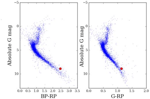
Hertzsprung–Russell diagram of stars in the NGTS field showing the position of NGTS J2143-38 above the main sequence. This suggests that it is likely a binary, as its position on the diagram makes it ∼ a factor of 2 more luminous than expected for a single star of similar spectral type.
The primary and secondary eclipses in the NGTS light curve are shown in Fig. 2 folded on the system period derived from global modelling. Note that the secondary eclipse is positioned close to phase 0.7, rather than the expected position of phase 0.5. Assuming that the light curve has been folded on the correct period, this shows that the system is in an eccentric orbit.

NGTS photometry of the primary and secondary eclipses of NGTS J2143-38 folded on a period of 7.618 d. The red line shows the model fit obtained from joint modelling of photometric and spectroscopic data.
2.2 SAAO photometry
NGTS J2143-38 was observed by the SAAO 1 m telescope on 2017 July 17. These observations were performed as part of the standard NGTS follow-up programmme. The aim of the observations was to confirm any transit and more accurately determine the transit depth and width. Observations were conducted over ∼5 h using the SHOC camera (Coppejans et al. 2013), in the z′ band.
The data were bias and flat-field corrected via the standard procedure, using the safphot Python package (Chaushev & Raynard, in preparation). Differential photometry was also carried out using safphot, by first extracting aperture photometry for both the target and comparison stars using the ‘sep’ package (Barbary 2016). The sky background was measured and subtracted using the sep background map, adopting box size and filter width parameters that minimized background residuals, measured across the frame after masking the stars. A 32 pixel box size and 2 pixel box filter were found to give the best results. Three comparison stars were then utilized to perform differential photometry on the target, using a 6 pixel radius aperture that maximized the signal-to-noise.
SAAO observations captured the bottom of the eclipse, as well as the egress and some out-of-transit flux of the primary star. They indicate a depth that is consistent with NGTS photometry, and that the eclipse occurred at a time consistent with the ephemeris from orion. The reduced light curve is shown in Fig. 3.
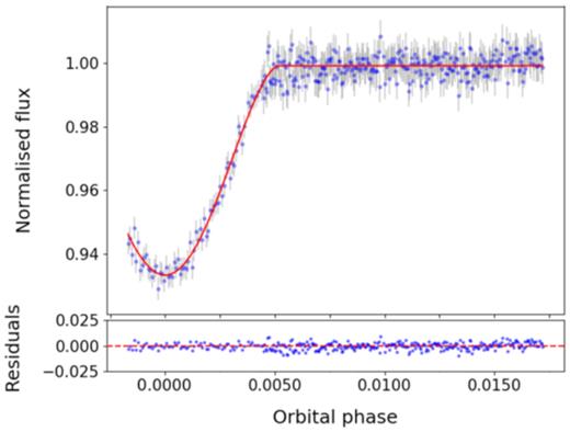
SAAO photometry of primary eclipse of NGTS J2143-38 plotted in phase. Observations were taken on the 1 m telescope using the z′ filter. The red line shows the model fit obtained from joint modelling of photometric and spectroscopic data.
2.3 TESS photometry
NGTS J2143-38 was observed by the TESS (Ricker et al. 2014) during Sector 1 of the mission. These observations occurred between 2019 July 25 and 2019 August 22. TESS observations typically consist of full frame images taken with 30 min cadence; however, 15 900 stars in Sector 1 were also observed at 2 min cadence by Camera 1, including NGTS J2143-38 (TIC ID = 197570458). The phase folded TESS light curve had a best BLS period of 7.618 725 d, consistent with the period determined from NGTS observations.
TESS captured three primary and two secondary eclipses of the system during this observation window. The phase folded TESS photometry also shows a secondary eclipse feature at phase 0.7, as in the NGTS photometry. The detection of this feature by two independent surveys confirms that the binary is in an eccentric orbit. The primary and secondary eclipses of the TESS light curve, folded on the period derived from global modelling (see Section 3.2), are shown in Fig. 4.
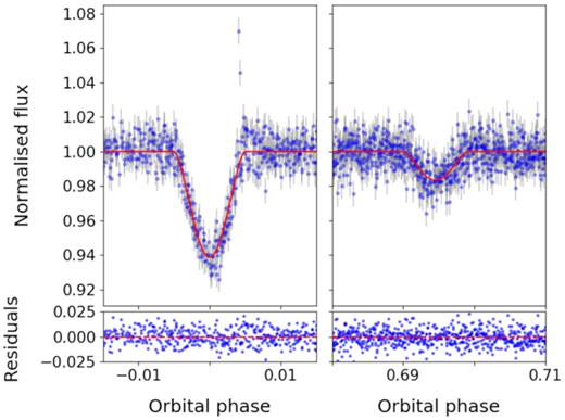
TESS photometry of primary and secondary eclipses of NGTS J2143-38 folded on the period of 7.618 d. The red line shows the model fit obtained from joint modelling of photometric and spectroscopic data.
2.4 HARPS and CORALIE spectra
NGTS J2143-38 was observed with the CORALIE spectrograph (Queloz et al. 2000) on the Swiss 1.2 m Leonhard Euler Telescope at ESO’s La Silla Observatory, Chile. The object is very faint for CORALIE (V = 15.39), so we took long (∼60 min) exposures to maximize the signal-to-noise ratio. This allowed for eventual precision in the RV measurement of around 250 ms−1 that is adequate for analysis of this system due to the high RV of the binary. We additionally obtained a single spectrum from HARPS (Mayor et al. 2003). We assume any systematic offset between the radial velocities for our instruments to be negligible given the magnitude of the RV shift that is expected from a binary of this type.
The spectra were cross-correlated with an M4 spectral mask and the cross-correlation function determined in order to derive the radial velocities of both stars. We determined which star each peak belonged to using the well-defined ephemeris from the previous photometric observations. We obtained a total of six observations spread across a full phase range that proved sufficient to constrain both the orbital eccentricity and masses of the system. The phase folded RV curve fit with our best model is shown in Fig. 5. The full RV measurements are given in Table 3.
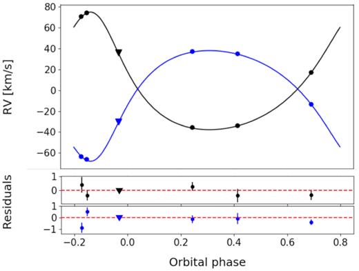
Phase folded radial velocity curve for NGTS J2143-38A (Black) and NGTS J2143-38B (Blue), with five radial velocity points taken by CORALIE (circles) and a single point obtained with HARPS (triangle). Radial velocities were phase folded on a period of 7.618 d. The black and blue lines show the model fit to the radial velocities obtained from global modelling of the system.
Radial velocities for NGTS J2143-38 A and B.
| BJDTDB | RV | RV error | FWHM | Contrast | Instrument |
|---|---|---|---|---|---|
| (−2,450,000) | (km s−1) | (km s−1) | (km s−1) | (per cent) | |
| STAR A | |||||
| 7958.810121 | 36.163 | 0.065 | 7.730 | 7.1 | HARPS |
| 7994.780464 | 17.437 | 0.370 | 7.911 | 7.4 | CORALIE |
| 8670.668149 | −33.780 | 0.490 | 6.900 | 6.1 | CORALIE |
| 8673.822407 | 70.990 | 0.570 | 4.600 | 2.6 | CORALIE |
| 8722.700796 | −35.54 | 0.320 | 8.164 | 7.0 | CORALIE |
| 8742.540179 | 74.4587 | 0.350 | 8.960 | 7.1 | CORALIE |
| STAR B | |||||
| 7958.810121 | −30.007 | 0.058 | 7.365 | 8.6 | HARPS |
| 7994.780464 | −13.217 | 0.250 | 7.448 | 8.3 | CORALIE |
| 8670.668149 | −35.000 | 0.480 | 8.400 | 7.1 | CORALIE |
| 8673.822407 | −63.178 | 0.440 | 4.700 | 3.8 | CORALIE |
| 8722.700796 | 37.210 | 0.330 | 8.642 | 7.5 | CORALIE |
| 8742.540179 | −65.785 | 0.375 | 9.787 | 7.6 | CORALIE |
3 ANALYSIS
3.1 Spectral typing
We obtained near-IR and visible spectra of NGTS J2143-38 using the X-SHOOTER instrument on ESOs VLT. The observations were taken as part of proposal 0101.C–0181 (characterizing M-dwarf exoplanet hosts and binaries from NGTS, Casewell PI).
NGTS J2143-38 was observed on the nights 2018 September 1 and 2. Observations were taken using the NIR and VIS arms of X-SHOOTER giving a wavelength coverage of 0.53–2.48 microns. We used an exposure time of 120 s, which resulted in a signal-to-noise ratio of >100 for the observations. The spectra were reduced and flux calibrated using the standard ESO X-SHOOTER pipeline (Modigliani et al. 2010).
These spectra were used to determine the spectral type of NGTS J2143-38. We first performed the telluric absorption correction on the spectra using ESO’s molecfit software (Kausch et al. 2015; Smette et al. 2015). Due to the high signal-to-noise ratio in our spectrum, we are able to perform these corrections without the need for telluric standard observations. In this case, molecfit uses a synthetic transmission spectrum determined by a radiative transfer code in order to perform the corrections.
The telluric-corrected spectra were then normalized at 1.2 μm and fitted to a variety of M-dwarf spectral templates, minimizing the sum of the squares of the difference between the model and real spectra. The best-fitting model spectrum was taken as the assumed spectral type of NGTS J2143-38. We used templates of M1 (HD24581), M2 (HD95735), M2.5 (Gl581), M3 (Gl388), M3.5 (Gl273), and M4 (Gl213) as detailed in Cushing, Rayner & Vacca (2005) and Rayner, Cushing & Vacca (2009). The best fit was obtained using a template of spectral type M3 (rms 0.078). The fit to each individual template spectrum, and the associated root-mean-square error, is given in Fig. 6.
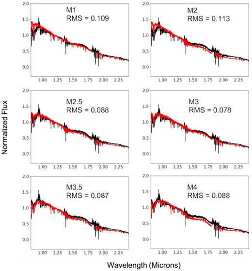
Telluric-corrected X-SHOOTER spectrum of NGTS J2143-38 (black) overlaid with template spectra for a range of M-dwarf spectral types (red). The root-mean-square error for each template is also shown. The best fit to a single spectrum is given by the M3 template.
3.2 Global modelling
To determine the masses, radii, and other parameters for the stars, we performed global fitting of both the photometric data (NGTS, TESS, and SAAO) and the RVs (CORALIE and HARPS). This was performed using the eclipsing binary light-curve simulation code ellc (Maxted 2016) in combination with the Markov chain Monte Carlo (MCMC) sampler emcee (Foreman-Mackey et al. 2013). Prior to the global modelling, the raw light curves were normalized by their median out of eclipse flux based on the ephemerides from orion. The NGTS data were binned to 2 min to reduce computational time.
We initialized the walkers in a region of parameter space that provided a good initial fit in order to save time. The starting position of each walker was selected from a normal distribution centred on these values. We used the values derived by orion to obtain initial values for both the transit epoch and the orbital period. Initial values for the primary star radius, stellar radius ratio, impact parameter, light ratio, and RV components were determined by first running the MCMC for a small number of steps to find values that gave a reasonable initial fit.
Limb darkening parameters were obtained using the ldtk software (Parviainen & Aigrain 2015). A quadratic limb darkening law was used with stellar properties, e.g. Teff and log g estimated based on the previously determined spectral type. Limb darkening coefficients and uncertainties were calculated directly with ldtk, for each photometric filter used, and placed as priors for the fitting process.
As we were unsure of the level of eccentricity of the system, although we expect it to be reasonably high given the position of the secondary eclipse, we initially set it to zero, and allowed the sampler to determine the level of eccentricity. We also incorporated an RV jitter term in our modelling to account for stellar noise, as well as normalization scaling parameters for each of the three light curves.
We used 200 walkers and 45 000 steps to model the light curve using the emcee sampler. Each walker used initial parameters that were randomized in a Gaussian ball around the values previously determined to give a good initial fit. We note that alterations to our initial values did not preclude the ability of the model to obtain a good fit, but did increase the burn in time required to do so. 10 000 steps were discarded as burn-in and not used when analysing the results of the modelling.
The parameters that obtain the best model fit to the overall data set are given in Table 4, and a corner plot showing the convergence of some key parameters is shown in Fig. 7. Our modelling gives best-fitting masses of MA = |$0.426 ^{+0.0056}_{-0.0049}$| M⊙, MB = |$0.455 ^{+0.0058}_{-0.0052}$| M⊙ and radii of RA = |$0.461 ^{+0.038}_{-0.025}$| R⊙, RB = |$0.411 ^{+0.027}_{-0.039}$| R⊙ suggesting a binary consisting of two roughly equal-sized early–mid M-dwarf stars. The stars are in a very grazing eclipse, with an inclination of 87.587° and impact parameter of 1.431. This leads to a sizeable uncertainty in the radii of the stars. Our global modelling also confirms the eccentricity of the system as suggested by both the photometry and RV measurements, with a value of 0.323. This leads to a pericentre distance of 10.615 R⊙ for the orbit.
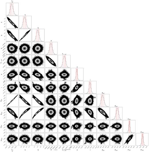
Corner plot showing the distribution of some key orbital parameters obtained from MCMC modelling of the system. Descriptions of each parameter are given in Table 4.
Fitted global modelling parameters and subsequent derived parameters for the NGTS J2143-38 system. The modal values of the posterior distributions were adopted as the most probable parameters, with the 68.3 per cent (1σ) highest probability density interval as the error estimates.
| Quantity | Description | Unit | Value | Error |
|---|---|---|---|---|
| Fitted parameters | ||||
| |$\frac{R_{\rm pri}}{a}$| | radius ratio of primary to semimajor axis | none | 0.029 52 | |$^{+0.002\,41}_{-0.001\,59}$| |
| k | radius ratio of stars, Rsec/Rpri | none | 0.891 66 | |$^{+0.108\,13}_{-0.142\,93}$| |
| b | impact parameter, cos (i)/Rpri | none | 1.430 83 | |$^{+0.088\,23}_{-0.116\,04}$| |
| |$\sqrt{e} \cos \omega$| | orbital eccentricity and argument of periastron term | none | 0.546 30 | |$^{+0.001\,17}_{-0.001\,41}$| |
| |$\sqrt{e} \sin \omega$| | orbital eccentricity and argument of periastron term | none | 0.148 21 | |$^{+0.009\,26}_{-0.008\,19}$| |
| P | orbital period | days | 7.617 93 | |$^{+0.000\,005\,16}_{-0.000\,005\,44}$| |
| Tc | epoch of primary eclipse centre | BJD | 2457501.97719 | |$^{+0.000\,40}_{-0.000\,39}$| |
| σNGTS | systematic error in NGTS light curve | norm. flux | 0.006 38 | |$^{+0.000\,0638}_{-0.000\,0627}$| |
| σz | systematic error in z’ light curve | norm. flux | 0.0002 32 | |$^{+0.000\,260}_{-0.000\,163}$| |
| σTESS | systematic error in TESS light curve | norm. flux | 0.002 83 | |$^{+0.000\,120}_{-0.000\,121}$| |
| βNGTS | normalized flux scale factor in NGTS data | none | 1.000 19 | |$^{+0.000\,0641}_{-0.000\,0655}$| |
| βz | normalized flux scale factor in z’ data | none | 0.999 13 | |$^{+0.000\,30}_{-0.000\,30}$| |
| βTESS | normalized flux scale factor in TESS data | none | 0.999 96 | |$^{+0.000\,0598}_{-0.000\,0635}$| |
| uNGTS-pri | linear LDC of primary in NGTS band | none | 0.485 71 | |$^{+0.032\,81}_{-0.032\,37}$| |
| |$u^{\prime }_{\rm {NGTS-pri}}$| | quadratic LDC of primary in NGTS band | none | 0.303 74 | |$^{+0.053\,51}_{-0.054\,03}$| |
| uNGTS-sec | linear LDC of secondary in NGTS band | none | 0.511 73 | |$^{+0.033\,12}_{-0.034\,37}$| |
| |$u^{\prime }_{\rm {NGTS-sec}}$| | quadratic LDC of secondary in NGTS band | none | 0.368 33 | |$^{+0.056\,81}_{-0.060\,64}$| |
| uz-pri | linear LDC of primary in z’ band | none | 0.349 17 | |$^{+0.036\,33}_{-0.036\,47}$| |
| |$u^{\prime }_{\rm {z-pri}}$| | quadratic LDC of primary in z’ band | none | 0.316 09 | |$^{+0.065\,49}_{-0.065\,55}$| |
| uz-sec | linear LDC of secondary in z’ band | none | 0.356 03 | |$^{+0.036\,79}_{-0.036\,93}$| |
| |$u^{\prime }_{\rm {z-sec}}$| | quadratic LDC of secondary in z’ band | none | 0.335 12 | |$^{+0.066\,36}_{-0.068\,34}$| |
| uTESS-pri | linear LDC of primary in TESS band | none | 0.467 57 | |$^{+0.032\,52}_{-0.032\,43}$| |
| |$u^{\prime }_{\rm {TESS-pri}}$| | quadratic LDC of primary in TESS band | none | 0.280 81 | |$^{+0.055\,62}_{-0.054\,39}$| |
| uTESS-sec | linear LDC of secondary in TESS band | none | 0.451 57 | |$^{+0.032\,78}_{-0.033\,32}$| |
| |$u^{\prime }_{\rm {TESS-sec}}$| | quadratic LDC of secondary in TESS band | none | 0.228 35 | |$^{+0.056\,51}_{-0.055\,40}$| |
| JNGTS | light ratio in NGTS band | none | 0.856 68 | |$^{+0.236\,97}_{-0.296\,01}$| |
| Jz | light ratio in z’ band | none | 0.682 00 | |$^{+0.200\,77}_{-0.247\,57}$| |
| JTESS | light ratio in TESS band | none | 0.778 50 | |$^{+0.204\,18}_{-0.247\,60}$| |
| Kpri | radial velocity semi-amplitude of primary | km s−1 | 56.480 61 | |$^{+0.304\,51}_{-0.287\,43}$| |
| Ksec | radial velocity semi-amplitude of secondary | km s−1 | 52.885 55 | |$^{+0.303\,85}_{-0.279\,38}$| |
| Γpri | systemic velocity measured from primary | km s−1 | 1.841 46 | |$^{+0.227\,79}_{-0.247\,78}$| |
| Γsec | systemic velocity measured from secondary | km s−1 | 1.948 10 | |$^{+0.219\,90}_{-0.224\,69}$| |
| σRV | jitter in RV data | km s−1 | 0.293 31 | |$^{+0.177\,64}_{-0.320\,47}$| |
| Derived parameters | ||||
| Rpri | radius of primary | R⊙ | 0.461 11 | |$^{+0.037\,95}_{-0.024\,92}$| |
| Rsec | radius of secondary | R⊙ | 0.410 60 | |$^{+0.026\,70}_{-0.038\,80}$| |
| mpri | mass of primary | M⊙ | 0.425 59 | |$^{+0.005\,58}_{-0.004\,91}$| |
| msec | mass of secondary | M⊙ | 0.454 51 | |$^{+0.005\,83}_{-0.005\,17}$| |
| a | semimajor axis of system | R⊙ | 15.618 05 | |$^{+0.064\,57}_{-0.056\,44}$| |
| i | orbital inclination | deg | 87.587 09 | |$^{+0.052\,65}_{-0.046\,50}$| |
| e | orbital eccentricity | none | 0.320 34 | |$^{+0.001\,20}_{-0.001\,17}$| |
| |$\log \, g_{\rm pri}$| | primary surface gravity | cm s−2 | 4.738 46 | |$^{+0.047\,97}_{-0.06808}$| |
| |$\log \, g_{\rm sec}$| | secondary surface gravity | cm s−2 | 4.867 71 | |$^{+0.087\,21}_{-0.054\,87}$| |
| T14-pri | primary eclipse duration | hours | 2.28084 | |$^{+0.028\,31}_{-0.041\,95}$| |
| T14-sec | secondary eclipse duration | hours | 2.30355 | |$^{+0.042\,17}_{-0.029\,87}$| |
3.3 Stellar rotation
In deriving the system parameters, we also attempted to determine rotation periods for the stars. From inspection of the TESS light curve, we see a clear sinusoidal-like variation that could be related to the rotation period of at least one of the stars. In order to fully characterize this, we ran a standard Lomb–Scargle period search to identify any periodic variations in the photometry. Prior to performing this, we removed the system’s primary and secondary eclipses from the photometry, to prevent periods based on these events from being detected.
We performed the Lomb–Scargle search on both the NGTS and TESS data. The periodogram for the TESS light curve is shown in Fig. 8. A clear peak can be seen with an associated period of 4.647 d. The NGTS light curve also shows similar periodic variability, with an identified period of 4.595 d. The identification of similar periodic variability in two independent sets of data is a strong indicator of validity.
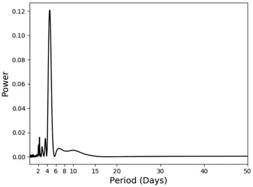
Lomb–Scargle periodogram for the TESS light curve after the removal of primary and secondary eclipse events. Note the strong peak at 4.647 d as a possible signature of stellar rotation.
The TESS light curve, folded on this suspected rotation period, is shown in Fig. 9. A clear sinusoidal variation at |$\sim 1{{\ \rm per\ cent}}$| level can be seen, which is likely associated with the rotation period of at least one of the stars. The NGTS light curve also shows some sinusoidal modulation; however, this is less noticeable than in the TESS data, due to the increased scatter of the data.
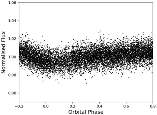
TESS light curve phase folded on a period of 4.647 d. Clear modulation can be seen with an amplitude of around 1 per cent, likely a signature of the rotation period of one (or both) of the stars.
3.4 SED fitting
In order to determine the effective temperatures of both stars, we fitted their spectral energy distributions (SEDs), following a method similar to Gillen et al. (2017). We fit both stars simultaneously using the PHOENIX v2 models (Husser et al. 2013). The PHOENIX models were initially convolved with our catalogue photometry to generate a grid of fluxes in Teff–log g space. This grid was then used to model the combined photometry of both stars. We fit for Teff, log g, and the radius R of each component, the distance D, along with an error inflation term, σ, which is used to account for underestimated catalogue uncertainties. To fully explore the posterior parameter space, we performed our fitting using an MCMC process using emcee (Foreman-Mackey et al. 2013). We used 200 walkers for 50 000 steps and used the final 10 000 to sample the posterior distribution. During fitting, we applied priors on the system distance and the radius of each component. We used a Gaussian prior for the system distance, using the Gaia DR2 measured value from Bailer-Jones et al. (2018). For the radius of each component, we used the measured values and uncertainties from our global fitting in Section 3.2, using two half-Gaussians for the prior distribution.
The fit to the system SED is shown in Fig. 10. From this, we derived effective temperatures of Teff = |$3452.97 ^{+56.34}_{-50.34}$| and |$3280.77 ^{+75.20}_{-126.74}$| K for the primary and secondary stars, respectively. This is in agreement with the temperature expected for two M3 dwarfs, and is consistent with the mass and radius derived from the global modelling of the system.
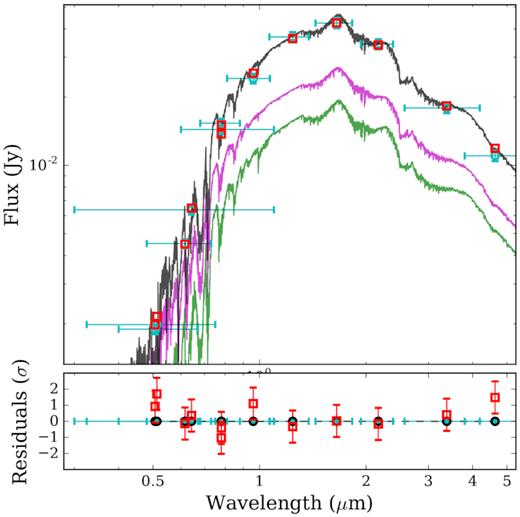
Upper panel – spectral energy distribution of NGTS J2143-38 fit with a combination of PHOENIX v2 model spectra (black line). The magenta and green lines show the individual model spectra for each star, and the blue points indicate the SED of the combined system. Lower panel – fit residuals for the combined spectrum.
4 DISCUSSION
4.1 Mass–radius relation
Since NGTS J2143-38 is in a grazing eclipse, there is a greater uncertainty in the masses and radii of the stars than there would be if the eclipses were to occur across the full face of each star. Nonetheless, as the stars lie in a parameter space with a relatively high number of measurements, we are able to compare our results to a large number of known systems, as well as to theoretical model predictions, to see where our stars fall among the already known significant scatter of the M-dwarf mass–radius relation.
Fig. 11 shows the mass and radius of the two stars plotted against model stellar isochrones from Baraffe et al. (2015). NGTS J2143-38B lies within 1σ of all model stellar isochrones, in agreement with model predictions for mass and radius. NGTS J2143-38A, however, appears to be inflated relative to its mass, differing from the model prediction for radius by almost 20 per cent.

Comparison between the two components of NGTS J2143-38 and the model stellar isochrones from Baraffe et al. (2015). A 0.5 Gyr isochrone is plotted in blue, a 1 Gyr isochrone is plotted in red, and a 5 Gyr isochrone is plotted in green. NGTS J2143-38A and NGTS J2143-38B are indicated by black triangles. Similar M-dwarfs from Parsons et al. (2018) are also plotted. The blue points are double-lined M-dwarf binaries, the red points are single stars, and the green points are M-dwarf secondaries in binaries with other spectral types.
When these stars are compared with the wider population of M-dwarfs, e.g. Fig. 11, we see that they lie within the expected scatter of M-dwarf uncertainty relative to theoretical relationships. However, the inflation of NGTS J2143-38A is still clearly visible, indicating that it is among the most inflated M-dwarfs known. From the known M-dwarfs shown in 11, it is apparent that the majority of outliers are also early–mid-type stars in M–M binary systems, with a configuration similar to NGTS J2143-38. As one of the most inflated systems, NGTS J2143-38 represents an excellent opportunity for investigating the underlying inflation mechanisms responsible for the oversizing observed in some M-dwarfs, and currently missing from physical models.
Boyajian et al. (2012) show that stars in eclipsing binaries have larger radii than single stars of the same temperature. This may be an explanation for the inflation seen in NGTS J2143-38A. It is perhaps slightly unusual, however, that only one of the stars shows this inflation, with NGTS J2143-38B showing reasonable agreement with model predictions. However, Kraus et al. (2017) report the discovery of an M-dwarf binary in which the primary star matches theoretical predictions whereas the secondary star is oversized relative to predictions. This is the opposite scenario to our system, in which the primary is inflated and the secondary is consistent with model predictions, which further highlights the complicated inconsistencies between models and predictions.
We note that while convention dictates that the primary star is defined to be that which gives the deepest eclipse when occulted by its companion (as in Gillen et al. 2017), this does not necessarily imply that the primary star is more massive than the secondary. Indeed, for NGTS J2143-38 we find the secondary star to be slightly larger in mass than the primary.
4.2 Mass-effective temperature relationship
We compare the effective temperatures for both stars derived in Section 3.2 to the known temperatures of the sample of M-dwarfs listed in Parsons et al. (2018). This is shown in Fig. 12, along with theoretical tracks (Baraffe et al. 2015) for stars of this mass range.
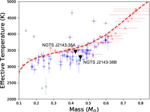
Mass–temperature relation for the sample of M-dwarfs given in Parsons et al. (2018). The components of NGTS J2143-38 are plotted in black, and a 5 Gyr isochrone is plotted in red for comparison. The blue points are double-lined M-dwarf binaries, the red points are single stars, and the green points are M-dwarf secondaries in binaries with other spectral types.
Like similar stars in this mass regime (see e.g. López-Morales 2007) both of our stars are cooler than model predictions by ≈100 K. This is consistent with the trend seen in partially convective stars, where luminosity (and hence temperature) is not strongly controlled by the conditions in their outer layers. Rather, the temperatures for these stars are affected by the conditions in the core. As seen in Fig. 12, lower mass (and hence fully convective) stars tend to agree better with model predictions, due to the fact that their luminosities are strongly determined by the conditions in the outer layers of the star.
4.3 Eccentricity
The global modelling of the system gives a value for the eccentricity of 0.323. This is unusual for M-dwarf binary systems that are often found in tight, almost perfectly circular orbits. Most double-lined eclipsing M-dwarf binaries with similar periods (such as Kraus et al. 2017; Orosz et al. 2012) show no such eccentricity in their orbits. LPSM J1112+7626 (Irwin et al. 2011) is an M-dwarf binary system with an eccentricity of 0.24; however, this system has a much longer orbital period (41.032 d) and as such a large level of eccentricity is less unusual.
There are some examples of eclipsing binaries with similar orbital periods that do exhibit some eccentricity. Triaud et al. (2017) obtained spectroscopic orbits of 100 low-mass eclipsing binaries with a range of orbital periods. Fig. 13 shows the eccentricity of these binary systems as a function of semimajor axis. While there are clearly examples of eccentricity in binary orbits with periods of the order of days, there are no examples of shorter orbital period binaries with greater eccentricity than NGTS J2143-38. It is also important to note that the objects in Triaud et al. (2017) are F-, G-, and K-type stars with M-dwarf secondary companions, and therefore do differ in nature to double M-dwarf binaries like NGTS J2143-38. Of the double-lined M-dwarf binaries listed by Parsons et al. (2018), none have a greater eccentricity than NGTS J2143-38, regardless of the period or semimajor axis of the systems.
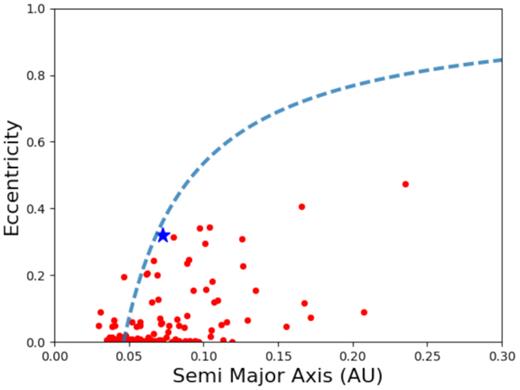
Plot illustrating the relationship between the semimajor axis of the binary and the eccentricity of the binary orbit for a sample of low-mass eclipsing binaries described in Triaud et al. (2017). NGTS J2143-38 is indicated in blue. A line of constant pericentre distance (10 R⊙) is shown in blue for comparison.
4.3.1 Tidal circularization
A possible explanation for this eccentricity may be that the system is rather young (<<1 Gyr). While tidal evolution of the binary may act to reduce the eccentricity of the orbit, there is no reason to expect the system to have began with little, or zero, eccentricity. If the system is sufficiently young that the eccentricity is yet to be reduced by these effects, then this may explain the presence of such a large eccentricity relative to the period of the orbit.
If this system is not young, then it is possible that tidal effects that would normally dampen the eccentricity of the system are not strong enough to do so in this scenario. We have already shown (in Fig. 13) that relative to its semimajor axis, NGTS J2143-38 has an extremely eccentric orbit. This makes the system a potentially useful test case for investigating the strength of tidal circularization effects in binary star systems.
Adopting a Q* value of 106 as has been assumed for some eclipsing binary and transiting exoplanet systems gives a circularization time-scale of 1.09 Gyr. As NGTS J2143-38 is in a highly eccentric orbit, it must clearly be younger than this, or its orbit would have had adequate time to circularize. However, previous studies cited by Penev et al. (2012) suggest that Q* could range anywhere between 105 and 109, and thus it remains extremely difficult to constrain the age of the system in this way. Thus, it is clear that either the system is significantly younger than 1.09 Gyr or alternatively Q* >> 106. If the age of the system were able to be determined, then tighter constraints on a value of Q* could be placed.
The age of this system is difficult to determine accurately. Stellar rotation rates from which the age can be inferred are difficult to determine for binary stars. Stellar activity can also be a useful indicator of age, as stars tend to be more active (and thus exhibit more flares) earlier in their evolution. We searched the light curve of NGTS J2143-38, which contained 139 nights of data spanning ≈7 months, and identified only two clear flare events in this time interval. This is likely just an indicator of the inherent activity of M-dwarf stars rather than a strong indicator of age. We also note that we examined the spectra of the system for Lithium absorption, a signature of young stars, and find no evidence of this. Additionally, the star does not appear to be part of a known moving group, from which its age could then be determined.
Zahn & Bouchet (1989) calculated a theoretical cut-off period, Pc, below which any binary system should have a circular orbit on the main sequence. For two stars with masses of 0.5 M⊙ with an initial eccentricity of 0.3, they give a cut-off period of 7.28 d. The components of NGTS J2143-38 are slightly less massive than this, and have a longer period, indicating that we may not expect this system to have been tidally circularized. Their determination that shorter period, more eccentric systems should not exist is supported by the fact that our system is of a longer period. They also determine that most tidal circularization occurs before the star joins the main sequence, and thus if our system is eccentric due to its age, then it must be very young.
4.3.2 Tidal synchronization
Additionally, to investigating the tidal circularization of the system, insight can be gained by considering the tidal synchronization of the system. As a binary star system evolves, the spin of the stars tends to be synchronized with the orbit due to tidal effects. The time-scale on which this occurs is much shorter than the time-scale required to circularize the orbit (Hurley et al. 2002), and thus investigating this effect could provide some insight into the age and evolution of the system provided we are able to determine a rotation rate for either of the stars.
In Section 3.2, we showed that there were periodic signals of 4.595 and 4.647 d from the NGTS and TESS data, respectively, which are likely related to the rotation period of at least one of the stars. Both of these periods, if they indeed correspond to the rotation of the stars, are significantly different from the orbital period of the binary. This implies that the system is not yet tidally spin–orbit synchronized. This would further the possibility that the system may be in the early stages of tidal evolution and thus the high level of eccentricity detected may not be entirely unexpected.
4.3.3 Possible tertiary companion
Anderson, Lai & Storch (2017) show that eccentricity in binary systems with periods of the order of days can be induced by the presence of a hidden tertiary companion to the binary. Assuming that the inclination between the orbits of the inner binary and the outer companion is sufficiently high, it is possible for the eccentricity to undergo periodic excursions to large values. These are known as Lidov–Kozai (LK) cycles (Kozai 1962; Lidov 1962).
It is believed that binaries with orbital periods shorter than around 7 d are not primordial, and that their current orbital configuration has evolved from a wider configuration perhaps due to these LK cycles (Mazeh & Shaham 1979; Eggleton & Kiseleva-Eggleton 2001; Fabrycky & Tremaine 2007; Naoz & Fabrycky 2014). It is indeed possible that this same interaction could induce the eccentricity that is seen in NGTS J2143-38. Tokovinin et al. (2006) observed a wide sample of spectroscopic binaries to search for higher order multiplicity. They found the presence of a hierarchical triple to be strongly dependent on the period of the binary orbit, with this being around 50 per cent for a 7 d period of the inner binary, as in our scenario. Therefore, it is a reasonable possibility that a tertiary component may be present in this system.
It is important to note, however, that the presence of a tertiary star does not guarantee that the binary eccentricity will be excited by these effects. It is strongly dependent on other factors, such as the orbital separation of the inner binary and the inclination between the orbits of the inner binary system and that of the tertiary star. Thus, we cannot conclude that NGTS J2143-38 has been raised to its eccentric orbit by these effects. We also note that there are no nearby Gaia DR2 sources in the vicinity of this object. The closest Gaia source is around 20 arcmin away, and is clearly not associated with this system based on its parallax and proper motion. From this, we can infer that any tertiary star is either too faint for Gaia or is too blended with NGTS J2143-38 to be resolved.
5 CONCLUSIONS
We report the discovery of an M-dwarf binary system NGTS J2143-38 using photometry from the NGTS. Follow-up observations allowed us to determine the masses and radii of the two stars, indicating a pair of roughly equal-sized M3 stars. Global modelling confirmed the eccentric nature of the system, and showed it to be the most eccentric M-dwarf binary known, and one of the most eccentric binaries of any type relative to its semimajor axis. Additional analysis of the system, including an accurate determination of the age, could provide interesting insights into the effects of tidal circularization in binary star systems.
ACKNOWLEDGEMENTS
Based on data collected under the NGTS project at the ESO La Silla Paranal Observatory. The NGTS facility is operated by the consortium institutes with support from the UK Science and Technology Facilities Council (STFC) project ST/M001962/1. This paper includes data collected by the Transiting Exoplanet Survey Satellite (TESS) mission. Funding for the TESS mission is provided by the NASA Explorer Program. This paper uses observations made at the South African Astronomical Observatory (SAAO). JA is supported by an STFC studentship. SLC acknowledges support from an STFC Ernest Rutherford Fellowship. RW and PW acknowledge support from STFC (consolidated grant ST/P000495/1). JIV acknowledges support of CONICYT-PFCHA/Doctorado Nacional-21191829. This project has also received funding from the European Research Council (ERC) under the European Union’s Horizon 2020 research and innovation programme (grant agreement no. 681601).
