


ABSTRACT
We determine the mass of the Milky Way bar and the torque it causes, using Gaia DR2, by applying the orbital arc method. Based on this, we have found that the gravitational acceleration is not directed towards the centre of our Galaxy but a few degrees away from it. We propose that the tangential acceleration component is caused by the bar of the Galaxy. Calculations based on our model suggest that the torque experienced by the region around the Sun is |$\approx 2400\, {\rm km^2\, s^{-2}}$| per solar mass. The mass estimate for the bar is |$\sim 1.6\pm 0.3\times 10^{10}\, \mathrm{M_\odot }$|. Using greatly improved data from Gaia DR2, we have computed the acceleration field to great accuracy by adapting the orbital Probability Density Function (oPDF) method (Han et al. 2016) locally and used the phase space coordinates of ∼4 × 10⁵ stars within a distance of 0.5 kpc from the Sun. In the orbital arc method, the first step is to guess an acceleration field and then reconstruct the stellar orbits using this acceleration for all the stars within a specified region. Next, the stars are redistributed along orbits to check if the overall phase space distribution has changed. We repeat this process until we find an acceleration field that results in a new phase space distribution that is the same as the one that we started with; we have then recovered the true underlying acceleration.
1 INTRODUCTION
Gaia satellite data releases allow us to construct quite detailed models for the Milky Way (MW) stellar density distribution and its kinematics. The latest Data Release 2 (Lindegren et al. 2018) gives us an excellent opportunity to explore the solar neighbourhood (SN) and somewhat more distant regions. In the present paper, we calculate the gravitational acceleration of the MW using the Gaia DR2 data, in an ellipsoidal region within a distance of 0.5 kpc from the Sun in the Galactic plane.
Modelling the MW is very different from modelling other disc galaxies since we make observations from within the MW. Although our location within the MW can make modelling easier, (e.g. individual stars are resolved) it can also add complications to it, e.g. dust attenuation and selection function can have a strong influence on modelling. For example, it was only at the beginning of the 1980s that the first direct hints that the MW may be a barred spiral galaxy came to light (Matsumoto et al. 1982). This was possible because of near-IR observations. Due to dust attenuation and our position inside the MW, it was difficult to draw such a conclusion on the morphology of MW before that.
On the other hand, we are at a great advantage because of the wealth of observational data available for the MW, unmatched and unavailable for other galaxies. For instance, axisymmetric models developed by Piffl et al. (2014), McMillan (2017), Binney & Wong (2017) use H i and CO velocities, maser data, Sgr A* proper motions, the globular cluster system, the velocity distribution in the SN, SDSS star counts in different colours, RAVE data, detailed MW satellite data and N-body simulation data. Additional constraints on the mass distribution were derived from cold stellar streams (Bovy et al. 2016) and Gaia DR2 proper motions of globular clusters (Watkins et al. 2019). However, the assumption of axisymmetry in mass distribution models is only a first approximation.
The existence of the central bar of the MW was first confirmed by Weiland et al. (1994), by analysing asymmetries in the near-IR surface brightness distribution of the central bulge from the COBE/DIRBE data. This was further confirmed by correcting the data for extinction (Dwek et al. 1995; Binney, Gerhard & Spergel 1997).
There are currently two contrasting scenarios – a fast rotating bar and a slow rotating bar. In the first case (e.g. Binney et al. 1997; Bissantz, Englmaier & Gerhard 2003; Monari et al. 2017) the bar is rotating with pattern speed |$\Omega _\mathrm{p} = 50\!-\!70\,\mathrm{km\, s^{-1}\, kpc^{-1}}$|; in the second case (Wegg & Gerhard 2013; Wegg, Gerhard & Portail 2015; Portail et al. 2015; Dias et al. 2019) the calculated pattern speed is |$25\!-\!30\,\mathrm{km\, s^{-1}\, kpc^{-1}}$|. Intermediate pattern speed values were derived by Li et al. (2016), Portail et al. (2017), Pérez-Villegas et al. (2017), Sanders, Smith & Evans (2019), Bovy et al. (2019) as |$\Omega _\mathrm{p} = 35\!-\!40\,\mathrm{km\, s^{-1}\, kpc^{-1}}$|. These calculated pattern speeds vary by about two times and as a result their corotation radii and outer Lindblad radii vary quite significantly. Both these scenarios agree that the angle between the major axis of the bar and the line connecting the Sun and the Galactic centre (GC) is about |$20\!-\!30\, \mathrm{deg}$|.
According to the axisymmetric models, the stars in orbits are phase-mixed. According to the non-axisymmetric models, stellar orbits are somewhat perturbed and phases of stars in orbits may not be completely mixed (Dehnen 2000; Fux 2001; Monari et al. 2017; Binney 2018; Trick, Coronado & Rix 2019) and thus orbital structure is more complicated (i.e. there are resonances). For example, using the Gaia DR2 data, Ramos, Antoja & Figueras (2018) found that, in the case of the MW, some orbit phases are mixed. Similar arcs and ridges were also found by Antoja et al. (2018), Kawata et al. (2018), Trick et al. (2019). Gravitational potential disturbances due to the bar may have caused deviations of stars from their initial orbits in the case of several cold stellar streams (Hattori, Erkal & Sanders 2016; Pearson, Price-Whelan & Johnston 2017; Banik & Bovy 2019) that originate from small stellar systems. The torque from the bar is not the only reason (see e.g. Kipper et al. 2019b). These disturbances can create observed gaps in stream surface density distributions.
Unfortunately, the structural parameters of the bar and its contribution to the gravitational acceleration are still rather poorly constrained. Thus, it is important to know the gravitational acceleration distribution in the Galactic plane and also to study how this allows one to constrain the bar properties. The Gaia satellite data provide an excellent opportunity to do this.
In the present paper we calculate all three acceleration components in the SN. We use the orbital arc method, developed in Kipper, Tempel & Tenjes (2019a). The method and its specific implementation details are described in Section 2. The method is used on the Gaia DR2 data. We use two different versions of the data, from the StarHorse project (Anders et al. 2019) and from the Schönrich catalogue (Schönrich, McMillan & Eyer 2019). The selection of the data used is described in Section 3. We demonstrate in Section 4 that the derived acceleration components cannot be explained within an axisymmetric model. The final section is dedicated to the summary and discussion.
We denote (x, y, z) as Galactocentric rectangular coordinates and (R, θ, z) as corresponding cylindrical coordinates, where θ = 0 corresponds to the opposite direction from the Sun. Transformations of sky coordinates, proper motions and radial velocities to Galactocentric coordinates and velocities were carried out using the astropy package (Astropy Collaboration et al. 2013; Price-Whelan et al. 2018). For the solar velocity, we used the values |$(\mathrm{U}_\odot , \mathrm{V}_\odot , \mathrm{W}_\odot) = (11.1,12.24,7.25)\, \mathrm{km}\, \mathrm{s}^{-1}$|, and Vg, ⊙ = Vc, ⊙ + V⊙, with the circular velocity |$V_{c,\odot } = 240\, \mathrm{km}\, \mathrm{s}^{-1}$| (López-Corredoira & Sylos Labini 2019).
2 METHOD AND IMPLEMENTATION
2.1 Orbital arc method
In this section, we provide a brief overview of the orbital arc method, which we have implemented in this paper to compute the gravitational acceleration, mass and torque estimates of the Galactic bar. For a detailed and thorough description of the formulation and tests of the model, please see Kipper et al. (2019a). We will refer to this particular method as the orbital arc method, since its most crucial step is the reconstruction of stellar orbits to accurately obtain the acceleration in the Milky Way, using the phase space information of stars. This has already been successfully applied to a simulation in Kipper et al. (2019a) and for the observational data in a simplified form (Kipper, Tempel & Tenjes 2018). Here we apply it for the Gaia DR2 data. The orbital arc method has five important steps.
Step 2 – Orbital arc reconstruction: Using the initial conditions, which is the phase space information from the data, and the acceleration field from the previous step, we solve the equations of motion to obtain stellar orbits for each star. A schematic of the reconstructed orbit arcs is represented as coloured arcs in Fig. 1.
Step 3 – Randomizing star position: The core of the proposed method lies in the oPDF, according to which the time of observing a star is random. This means that we can reposition a star along its orbit by picking a random time from a uniform distribution of time. By picking infinitely many times from this distribution, we reach a continuous distribution of the star along its orbit (a similar description to the procedure can be found in Han et al. 2016). Following this, we reposition every star in its orbit and get a new distribution of stars in the region. This is relevant in the last step where we will compare the old and new distributions.
Step 4 – Phase space density: In order to compute the probability of finding a star in its orbit, we need to first specify a small segment of the star’s orbit. For this, we construct Voronoi tessellations by considering small subsets of data, such that in each Voronoi cell there are similar numbers of stars; this reduces the Poisson error. The Voronoi cells are shown in the schematic diagram in Fig. 1. To compute the probability of finding a star in its orbit, we use the Voronoi cells as the orbital segments. For example, for star 1 in Fig. 1, the time spent by the star in each Voronoi cell along its orbit is given as Δti. So, the probability of finding that star in the ith Voronoi cell is the time spent in that Voronoi cell, Δti, divided by the time spent in the entire region, which is, Δti/(texit − tenter) as seen in Fig. 1. Eventually, a combined probability is calculated for each Voronoi cell, which is the sum of probabilities of all stars in each cell.
Step 5 – Comparing phase space density distributions: In this final step we compare the phase space distribution of the original data and the phase space distribution of the newly positioned stars. The phase space distribution comparison is done statistically by computing the likelihood. If the likelihood is not maximum then the entire process is repeated with new acceleration field parameters.
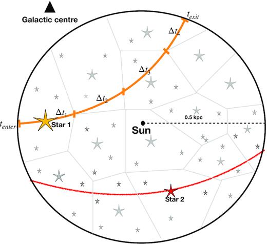
An illustration of the region where the orbital arc method is applied. The central point represents the Sun and the circular region up to a distance of 0.5 kpc from the Sun is the region used in this paper. The black triangle points towards the Galactic centre. The coloured arcs for star 1 and star 2 represent the reconstructed orbits for these two stars. Orbital arcs are reconstructed for all stars in this region. The grey cells are the Voronoi cells, each of which contains a similar number of stars. The time interval, Δti, is the time a star spends in the ith Voronoi cell. The times at which the star enters and exits the region are tenter and texit, respectively.
Eventually, the orbital arc method will give the acceleration field corresponding to the maximum likelihood, which is the field that describes the true underlying acceleration of the MW. The distribution of likelihoods gives the statistical uncertainty.
Since the level of accuracy relies on the available data, we need the phase space coordinates of a sufficiently large number of stars. Hence, Gaia DR2 is aptly suited for the study.
2.2 Implementation: the smoothing kernel
In order to compare the phase space distributions of the original data and the repositioned stars, we have used Voronoi cells to get a smooth phase space density. This is achieved by computing the time stars spend in each Voronoi cell, as described in step 4 in Section 2.1. In Fig. 1, Δt represents the time a star spends in a cell. The ratio of the time spent by a star in a Voronoi cell, Δti, to the time that it spends in the entire region (see tenter and texit in Fig. 1) gives the phase space density of this model.
The shapes and sizes of the regions in which we intend to calculate the accelerations are mainly motivated by the quality of 6D data. The shapes of these regions and the Voronoi cells used to smooth phase space1 should be complementary to each other. For example, if the available data are of a spherical region, then a rectangular grid or cell is not the most optimal. Therefore, the best possible grid should coarsely follow the distribution of data. One of the best ways to achieve this is by Voronoi tessellations, and we have hence used this method for the paper. However, in principle, any similar grid can be used. We used a random small subset of the data of about ∼100 stars to obtain the Voronoi cells.
Each grid-cell is described by two numbers: the closest tessellation centre in ordinary space and the closest tessellation centre in velocity space. These two indices are required to avoid combining velocity and distance data into a single quantity, because this kind of combination produces an additional free parameter that we wish to avoid. For example, by using 100 data points to tessellate into a grid, we will have |$100^2 = 10\, 000$| independent cells, which is usually sufficient to describe the phase space distribution of about |$\approx 420\, 000$| stars (i.e. 42 stars per cell). For the current study, we have selected 100 cells for each of position and velocity space, unless noted otherwise.
2.3 Implementation: flux limitedness
Flux-limited observational data are a natural constraint in large surveys. There are two common approaches to overcome this: a) to construct a volume-limited sample and discard some data, or b) to use all the data and add a weight to each point.
Most dynamical modelling methods are constructed based on the assumption that we are able to observe everything, i.e. the volume-limited approach. Some specifics of the present modelling allow us to use the advantage of increased amounts of data of the flux-limited selection, while essentially using the method constructed for the volume-limited approach. This approach is described further in this section.
2.4 Requirements for data
An integral part of the method is orbit calculation. This has two ingredients: the proposed acceleration function and initial conditions for the orbits. As an analytical expression the first one is infinitely precise for each likelihood evaluation. The second one is as precise as the data allow. Imprecisions in the data are amplified by the orbit integration, i.e. Δx ∼ Δx0 + tΔv, where Δ denotes uncertainty for positions and velocities respectively. This shows that the uncertainties accumulate with time; hence the position of a star is unknown in some cone. Due to uncertainties (especially heteroscedastic ones) in the Gaia data combined with smoothing phase space, we may reconstruct imprecise orbits, which will introduce a bias in the acceleration. The simplest way to avoid these problems is to use maximally precise data.
The second requirement is to have a sufficient amount of data. This is needed to describe the phase space density sufficiently precisely. Assuming that the data are very precise, the only source of uncertainty is the Poisson noise from the sampling.
3 OBSERVATIONAL DATA
3.1 Construction of the data sample
Six-dimensional high-quality phase space coordinates in the SN are now available from the Gaia satellite Data Release 2 for a significant number of stars. At present there are three catalogues available based on the Gaia measurements and including estimated star distances: the Gaia Collaboration catalogue (Lindegren et al. 2018), the StarHorse project catalogue, SH (Anders et al. 2019) and the Schönrich catalogue, Sc (Schönrich et al. 2019). There is a known issue concerning the zero point of parallaxes from the Gaia Collaboration, which is overcome in the latter two catalogues. Therefore we selected these two catalogues as our main sources of input data and calculated our results for both of them separately. To calculate gravitational acceleration, we need to know mass density gradients. Although the main source of density gradients results from the smooth density distribution of the MW, selection effects can produce artificial gradients. The two dominant ingredients for this kind of selection effects are Malmquist bias (covered in the previous section) and dust attenuation. To suppress the effects from dust attenuation, we use 2MASS (Skrutskie et al. 2006) catalogue J-band magnitudes where extinction is negligible.
The cross-match between the Anders et al. (2019) SH and 2MASS catalogues gave 6964 515 entries; between the Schönrich et al. (2019) Sc and 2MASS catalogues there were 6519 209 matches. We constrained the input magnitudes in such a way that the Gaia G-band completeness (being affected by dust attenuation) has substantially less effect than our selection based on the J passband (being nearly attenuation free), i.e. P(G > Glim|J < Jlim) ≪ 1. The apparent-magnitude data within 0.5 kpc from the Sun for our selected sample are shown in Fig. 2. A strong correlation between the G- and J-band magnitudes catches the eye. The J-band limit Jlim was fixed to a value where the distribution of brighter stars in the G band ends before reaching the Gaia spectroscopic completeness limit Glim. This is shown as a green line in the left-hand panel and the corresponding probability density distribution p(G|J < Jlim)dG in the right-hand panel. The fraction of G magnitudes crossing Glim is 8 × 10⁻⁴ for the adopted Jlim = 10.25; hence we conclude that our sample is almost independent of the Gaia completeness limit and dust attenuation.
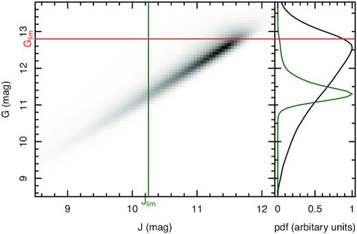
Distribution of apparent magnitudes of all stars within 0.5 kpc from the Sun. The G-band magnitudes are from the Gaia data and the J-band magnitudes are from the 2MASS survey. The red horizontal line and the green vertical line depict the spectroscopic completeness limit and the limiting magnitude Jlim, respectively, of our main sample. The right-hand panel shows the distribution of all stars from Gaia. The black line shows all the stars and the green line shows only those with magnitudes brighter than Jlim. The distribution of our sample of stars drops before reaching the Gaia completeness limit. Only a fraction of 0.0008 stars have a higher G-band magnitude; therefore we choose our sample based on 2MASS photometry.
The smooth acceleration distribution of the MW is taken as an input in modelling process and it does not include local potential wells of stellar clusters. Hence, we cannot describe the motion of stars within clusters and must exclude these cluster stars from our sample. We excluded all stars that appeared to be cluster members in catalogues by Cantat-Gaudin et al. (2018) or the Gaia Collaboration et al. (2018). In total, 993 stars or about 0.2 per cent of stars from the final selection were excluded.
3.2 Selection of the region
In the paper where we presented the method and tested it on simulation data (Kipper et al. 2019a), we aimed to use rather small regions in order to have a simple analytical form for acceleration vector components. In the current paper, we selected a larger region to suppress Poisson noise and to increase the region size in the radial direction to have a stronger basis to also estimate the first derivative of the radial acceleration. This changes our approach somewhat: instead of using a simple form for accelerations, we now try to model the underlying acceleration field with a well-motivated analytical form.
Thus, due to available data, instead of using several small regions as we did in Kipper et al. (2019a), we selected one larger region, as shown in the schematic in Fig. 1. Our main aim was to recover the acceleration field in the plane of the Galaxy; hence we constructed a region where accelerations in the MW plane have a longer time to act on stars. In the vertical direction, density gradients are much steeper and one may expect that the corresponding accelerations may have also more complex forms. To avoid using more complex accelerations in vertical directions, we selected a thin region.
4 RESULTS
We calculated gravitational acceleration in the region around the SN as described in Section 3.2 using the method and its implementation explained in Section 2. In order to decipher various aspects of the acceleration field (e.g. deviations from axisymmetry), we used different functional forms to describe the underlying acceleration.
4.1 Calculated acceleration components
In our first attempt to model the acceleration in the region we did not specify a design-based form of an overall gravitational potential of the MW. Instead we assumed that any acceleration form can be approximated with their Taylor expansions equations (7)–(9) and we fit the coefficients of this acceleration (Ax, Ax, x, Ax, y, Ax, z, Ay, Ay, x, Ay, y, Ay, z, Az, Az, x, Az, y, Az, z). This way of modelling is powerful because it allows us to not only model the acceleration in a tiny region, but in principle the entire MW if we can get the overall gravitational potential. We fit a total of 12 free parameters, Ai and Ai, j for the flux-limited samples of stars within the selected region (see Section 3.2) for both the Sc and SH catalogues of Gaia DR2 (for more details see Section 3.1).
We used 100 random points to describe the grid; hence, there are ≈42 stars per grid bin. The fitting was done with the multinest code (Feroz & Hobson 2008; Feroz, Hobson & Bridges 2009; Feroz et al. 2013) using 500 live points. To include the randomness caused by the gridding, we ran the code eight times and averaged the posterior distribution of different runs. All the modelling was done in this way, unless noted otherwise. The priors of the Bayesian modelling were chosen to be of uniform distribution with the limiting values provided in Table A1. In the table we give the posterior distribution of each parameter ζ with five quantiles positioned at P(ζ) = {0.023, 0.159, 0.500, 0.841, 0.977}.
Previous studies have shown that the Sun is not located precisely at the centre of the Galactic plane, but is about |$25\, {\rm pc}$| away from it (Bland-Hawthorn & Gerhard 2016). Thus, there must be an acceleration component in the vertical direction, as confirmed in e.g. Kipper et al. (2018) based on dynamics. In Table A1 our estimation of the vertical acceleration Az and its gradient in the z-direction Az, z are given. Using these two values and by making a linear approximation at distances close to the plane, we deduce that we are located at |$\mathrm{z}_\odot \approx A_z/A_{z,z} = \lbrace -111^{+33}_{-76} ({\rm SH}),\, -117^{+58}_{-66} ({\rm Sc})\rbrace$| pc from the vertical coordinate value defined as having zero vertical acceleration in contrast to the symmetry-defined centre.
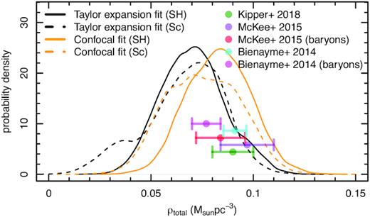
The figure shows the average matter density in the solar neighbourhood and is compared with the results from Bienaymé et al. (2014), McKee, Parravano & Hollenbach (2015), Kipper et al. (2018). These results do not match very well because they use different datasets and different assumptions of the underlying acceleration. The high uncertainty in the calculated results is due to the optimization of the selected acceleration form to determine accelerations in the Galactic plane. Note that this is not the vertical component, which is usually used to determine the overall matter density.
4.2 Deviations from a simple axisymmetric MW model
In case of a stationary axisymmetric MW, the acceleration component along the direction of Galactic rotation ay(Δx, Δy = 0, Δz) = 0 and equipotential curves are concentric circles. The median values of acceleration computed within the selected region using the coordinates (x, y, z) = (− 8.3, 0, 0) kpc as the centre are 306 and |$284\, {\rm km^2\, s^{-2}\, kpc^{-1}}$| for the SH and Sc catalogues respectively. Results of these calculations along with 1σ and 2σ limits are shown in Fig. 4 and the used priors are given in Table A2. They are designated as ‘Sc, flux’ and ‘SH, flux’. None of the |$27\, 748$| posterior samples from multinest show negative Ay values. Thus, the results are not consistent with axisymmetry.
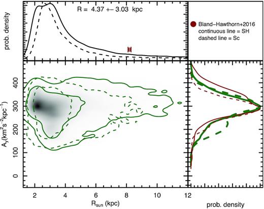
The central panel shows the correlation between the centre of acceleration, R⊙, and the component of the acceleration vector, Ay, as described in Section 4.2. The top panel shows the distribution of R⊙ for an axisymmetric fit. The brown point at 8.3 kpc shows the distance of the Sun to the centre of our Galaxy. This indicates that the curvature of the isopotential lines is very likely less than 8.3 kpc. The right-hand panel shows the distribution of the Ay component of the acceleration vector at the region centre. The green lines are for the overall posterior distribution and the red lines are for the subset where |$\mathrm{R}_\odot \approx 8.3\, {\rm kpc}$|. This figure highlights the necessity to include the non-axisymmetric component to fit the acceleration, since the default for the MW at (R⊙ = 8.3, Ay = 0) does not account for what is observed.
Based on the assumption that equipotential curves are concentric circles, we derived the radius of this circle. The radii are |$3.4\, {\rm kpc}$| for the SH catalogue and |$3.2\, {\rm kpc}$| for the Sc catalogue. Most of the posterior distribution had values lower than 8.3 kpc, i.e. |$P(\mathrm{R}_\odot \,\gt \,8.3\, {\rm kpc}) = \lbrace 0.048 ({\rm Sc}),\, 0.11 ({\rm SH}) \rbrace$|. Hence, the ‘acceleration centre’ is most likely closer to us than the GC and equipotential curves have higher curvature than one would expect for the distance to the Galactic centre. Thus we conclude that axisymmetric potential distribution is not valid at SN, and interpret it as an argument to support the presence of a rather massive central bar.
As already explained in Section 5.1, we calculated the acceleration components assuming axisymmetry, by selecting the components aR, az to be in the form of equations (4)–(6). During the fitting the solar distance R⊙ was also taken as a free parameter. Taking the posterior in these fits close to |$\mathrm{R}_\odot =8.3\, \mathrm{kpc}$|, we found the radial acceleration to be |$-6190^{+70}_{-160}\, {\rm km^2\, s^{-2}\, kpc^{-1}}$|, which corresponds to the circular velocity 227 km s−1. The combined estimate of the observed circular velocity at 8.3 kpc is somewhat larger, being |$238\pm 15\,{\rm km\, s^{-1}}$| (Bland-Hawthorn & Gerhard 2016), but it is consistent with the calculated result within error.
4.3 Deriving the properties of the bar
When using accelerations in the form of equations (16)–(18), substantial correlations exist in the modelled posterior samples (e.g. between Ar and Ar, bar). The largest correlation coefficient was found to be 1.0 between Ar and Ar, bar (see Fig. 5). We also found a strong correlation (correlation coefficient 0.85) between bar acceleration/total acceleration and its focal length as shown in Fig. 6. The rest of the correlations were much weaker, and the only other noticeable correlation was between AR and AR, bar and the radial acceleration derivative AR, R (correlation coefficient 0.26).
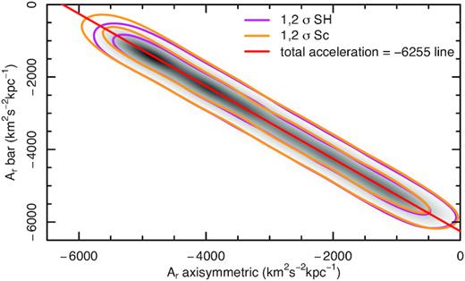
The relation between acceleration from the axisymmetric component and from the bar component. The contours show 1σ and 2σ confidence intervals for the Anders et al. (2019) (SH) and Schönrich et al. (2019) (Sc) datasets. The strong correlation between them shows degeneracy of accelerations in the functional form of equations (16)–(18).
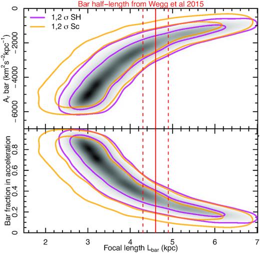
The top panel depicts the degeneracy between the length of the bar and the acceleration from it. The bottom panel shows the fraction of bar acceleration. The degeneracy can be broken when additional information such as bar length is used. We used the bar length value from Wegg et al. (2015). The contours show 1σ and 2σ confidence intervals for the Anders et al. (2019) (SH) and Schönrich et al. (2019) (Sc) datasets.
Currently we have only used the SN region to disentangle the bar parameters; hence, we were able to determine only some of the degenerate values. We were also able to determine that the sum of the radial acceleration due to the bar and axisymmetric components is constant, as seen in Fig. 5. Hence, if we know one then we can easily estimate the other.
5 DISCUSSION AND CONCLUSION
5.1 Validity of the sample construction
To test how well the approach described in Section 2.3 is able to cope with flux-limited data, we applied our model to two sets: a flux-limited sample and a volume-limited sample. The volume-limited approach was tested with simulation data in Kipper et al. (2019a) and was found to be consistent. Since the results for the flux-limited sample agreed well with those of the volume-limited sample, we are confident that our model is very suitable for the current case.
The acceleration components used for this test are in the axisymmetric form of equations (4)–(5). The geometry of the region was biaxial ellipsoid in the form of equation (12), but its selection and modelling had some differences: the sample was limited by the absolute J-magnitude value of 1.2m, yielding |$54\, 819$| stars. The grid was constructed by using 70 random sample points, and fitting was done eight times to include the uncertainty from the gridding randomness.
The results of the test calculations for volume- and flux-limited selections from the Sc catalogue are given in Table A2, where calculated acceleration components are given with labels ‘Sc, vol’ and ‘Sc, flux’. The most interesting acceleration components are radial acceleration aR and vertical acceleration az (see their main parameters AR and Az). For the volume-limited sample |$A_R = -6128 \pm 199\, {\rm km^2\,s^{-2}\, kpc^{-1}}$| and |$A_z = 183 \pm 106\, {\rm km^2\,s^{-2}\, kpc^{-1}}$|; for the flux-limited sample |$A_R = -6181 \pm 82\, {\rm km^2\,s^{-2}\, kpc^{-1}}$| and |$A_z = 203 \pm 48\, {\rm km^2\,s^{-2}\, kpc^{-1}}$|. The smaller errors in the flux-limited sample are due to the larger data sample. The results are clearly consistent and we may conclude that our approach to cope from here on with the flux-limited sample, described in Section 2.3, is valid.
5.2 Time dependence of acceleration due to the bar
During calculations of stellar orbits (see selected analytical forms for acceleration) we assume that accelerations do not have an explicit time dependence. However, it is known that about a quarter of galaxies contain a more or less prominent bar (Cheung et al. 2013); in the case of the MW a central bar was introduced by de Vaucouleurs (1964). A rotating bar would violate this assumption of our modelling.
To test how much a bar would influence our results, we used the same simulation (the barred one) from Garbari, Read & Lake (2011) as was used in Kipper et al. (2019a). We selected a region close to the solar radius, with an angle between the major axis of the bar and direction to the centre of the region ≈30° and fitted the acceleration components (7)–(9) (Taylor expansion) with our model. We expect that including the tangential component of the acceleration due to the bar that is changing in time would give us a somewhat wrong acceleration direction. We found that the acceleration vector was directed away by 3.27 ± 2.23° from the Galactic centre. The corresponding true angle calculated directly from the simulation gravitational potential was 2.21°. The difference between the true and calculated values is smaller than the 1σ error of the calculated value. Hence the effect of the time dependence of the bar in this case is not so significant.
5.3 Influence of uncertainties in input data
The input to this modelling does not include uncertainties. The resulting uncertainties are statistical in nature and include only sampling errors seen from the likelihood equation (7) of Kipper et al. (2019a). In order to see how observational uncertainties influence our results, we randomized phase space coordinates of stars according to their uncertainties, reconstructed the selection sample as described in Section 3, and remodelled the selected region. To account for the randomness in this process, we modelled the SN 47 times and combined the corresponding posterior distributions. The results of the calculations are shown in Table A2 with the label ‘Sc, rnd’ after the variable name. Comparing calculated accelerations with labels ‘Sc, rnd’ and ‘Sc, flux’, it is seen that randomization had very little effect on the results. We conclude that uncertainties can be ignored for this selection.
Another source of error can be due to the gridding approach employed in this study (see Section 2.2). Since there is randomization, we must include the noise caused by it. We rerun each modelling eight times to include the source of noise. All of these runs had similar posterior distributions; hence we are certain that gridding does not introduce large artificial uncertainties. To include the gridding uncertainties, we combined the posterior distributions of randomized grid runs.
5.4 Conclusions
In this paper, we have applied the orbital arc method (Kipper et al. 2019a) to Gaia DR2 and modelled the acceleration along the plane of the Galactic disc. We approximated the acceleration in the solar neighbourhood with various functional forms and came to the following conclusions:
There are very few systematic biases between the Gaia DR2 datasets compiled by Schönrich et al. (2019) and Anders et al. (2019). Both the datasets give consistent results.
The distribution of axisymmetric gravitational acceleration does not account for the observed acceleration for the standard distance of the Sun from the Galactic centre |$\mathrm{R}_\odot \approx 8.3\, {\rm kpc}$|. The curvature of the isopotential lines is smaller than the standard R⊙, implying that there is a component of the Galactic bar causing this acceleration.
The acceleration vector in the solar neighbourhood is not directed towards the centre of the Galaxy. There is a significant component of the acceleration directed away from the Galactic centre. We propose that this is caused by the massive central bar. Based on our model, we calculate the torque to be |$\sim 2400\, {\rm km^2\, s^{-2}}$| per solar mass.
Based on the assumption that isopotential surfaces of the bar are confocal ellipses, we estimate that about a third of the total acceleration in the solar neighbourhood is caused by the bar. In this computation we use the estimate of the length of the bar of Wegg et al. (2015).
Finally, using our model, we estimated the mass of the bar as |$(1.6\pm 0.3)\times 10^{10}\, \mathrm{M}_\odot$|, using the density distribution parameters from Wegg et al. (2015).
ACKNOWLEDGEMENTS
We thank the referee for helpful comments and suggestions. We thank the StarHorse core team (F. Anders, A. Queiroz, B. Santiago, A. Kalathyan, C. Chiappini) for providing their data, and G. Monari for helpful comments about the paper. This work was supported by institutional research funding IUT26-2, IUT40-2 and PUTJD907 of the Estonian Ministry of Education and Research. We acknowledge the support by the Centre of Excellence ‘Dark Side of the Universe’ (TK133) and by the grant MOBTP86 financed by the European Union through the European Regional Development Fund. This work has made use of data from the European Space Agency (ESA) mission Gaia (https://www.cosmos.esa.int/gaia), processed by the Gaia Data Processing and Analysis Consortium (DPAC, https://www.cosmos.esa.int/web/gaia/dpac/consortium). Funding for the DPAC has been provided by national institutions, in particular the institutions participating in the Gaia Multilateral Agreement. This publication makes use of data products from the Two Micron All Sky Survey, which is a joint project of the University of Massachusetts and the Infrared Processing and Analysis Center/California Institute of Technology, funded by the National Aeronautics and Space Administration and the National Science Foundation.
Footnotes
The Voronoi tessellation of the region is done in order to compare the original and new phase space distributions.
We make an approximation that the mass of the bar is a point mass at the tip of the bar. This gives an upper limit for the bar influence.
REFERENCES
APPENDIX A: TABLES
The modelling of the acceleration function described with equations (7)–(9) and using datasets from Schönrich et al. (2019) (Sc) or Anders et al. (2019) (SH). We use acceleration units of |${\rm km^2\, s^{-2}\, kpc^{-1}}$|, which differ from the more intuitive |${\rm km\, s^{-1}\, Gyr^{-1}}$| by about 2 per cent. The values of P represent quantiles of the posterior distribution.
| Variable | Unit | P = 0.02 | P = 0.16 | Median | P = 0.84 | P = 0.98 | Lower prior limit | Higher prior limit |
|---|---|---|---|---|---|---|---|---|
| Ax (SH) | km2 s−2 kpc−1 | 6109.43 | 6178.27 | 6250.33 | 6382.74 | 6468.32 | −10 000 | 10 000 |
| Ax (Sc) | km2 s−2 kpc−1 | 6026.12 | 6102.47 | 6195.79 | 6327.5 | 6420.91 | −10 000 | 10 000 |
| Ay (SH) | km2 s−2 kpc−1 | 222.24 | 259.31 | 306.37 | 385.33 | 445.89 | −10 000 | 10 000 |
| Ay (Sc) | km2 s−2 kpc−1 | 189.42 | 238.87 | 283.55 | 339.59 | 412.18 | −10 000 | 10 000 |
| Az (SH) | km2 s−2 kpc−1 | 138.96 | 175.95 | 211.06 | 254.66 | 295.01 | −5000 | 5000 |
| Az (Sc) | km2 s−2 kpc−1 | 95.85 | 135.28 | 186.81 | 245.17 | 286.13 | −5000 | 5000 |
| Ax, x (SH) | km2 s−2 kpc−2 | 252.69 | 658.7 | 1152.87 | 1764.86 | 2306.3 | −3000 | 5000 |
| Ax, x (Sc) | km2 s−2 kpc−2 | −498 | 318.77 | 1109.62 | 1631.22 | 2088.79 | −3000 | 5000 |
| Ax, y (SH) | km2 s−2 kpc−2 | −34.2 | 853.24 | 1867.96 | 2920.27 | 3606.84 | −4000 | 4000 |
| Ax, y (Sc) | km2 s−2 kpc−2 | −479.88 | 494.3 | 1511.29 | 2379.45 | 3128.42 | −4000 | 4000 |
| Ax, z (SH) | km2 s−2 kpc−2 | −1948.43 | −1760.52 | −1406.23 | −860.97 | −171.53 | −2000 | 2000 |
| Ax, z (Sc) | km2 s−2 kpc−2 | −1945.27 | −1748.13 | −1339.24 | −725.73 | 2.09 | −2000 | 2000 |
| Ay, x (SH) | km2 s−2 kpc−2 | −702.07 | −424.69 | −59.88 | 253.95 | 538.2 | −2000 | 2000 |
| Ay, x (Sc) | km2 s−2 kpc−2 | −541.84 | −283.02 | −28.31 | 275.48 | 640.52 | −2000 | 2000 |
| Ay, y (SH) | km2 s−2 kpc−2 | −3505.68 | −2862.34 | −2148.94 | −1487.17 | −935.21 | −5000 | 2000 |
| Ay, y (Sc) | km2 s−2 kpc−2 | −3662.39 | −2914.14 | −2154.12 | −1566.75 | −933.65 | −5000 | 2000 |
| Ay, z (SH) | km2 s−2 kpc−2 | −1975.02 | −1885.74 | −1696.72 | −1372.29 | −860.07 | −2000 | 2000 |
| Ay, z (Sc) | km2 s−2 kpc−2 | −1957.05 | −1817.54 | −1463.88 | −864.12 | −129.38 | −2000 | 2000 |
| Az, x (SH) | km2 s−2 kpc−2 | −494.93 | −145.76 | 155.8 | 428.63 | 700.61 | −2000 | 2000 |
| Az, x (Sc) | km2 s−2 kpc−2 | −48.17 | 184.64 | 429.13 | 669.57 | 906.36 | −2000 | 2000 |
| Az, y (SH) | km2 s−2 kpc−2 | −636.93 | −50.74 | 562.24 | 1220.58 | 1772.55 | −2000 | 2000 |
| Az, y (Sc) | km2 s−2 kpc−2 | −304.58 | 102.45 | 501.94 | 893 | 1284.27 | −2000 | 2000 |
| Az, z (SH) | km2 s−2 kpc−2 | −3066.65 | −2536.04 | −1857.43 | −1224.14 | −664.61 | −6000 | 0 |
| Az, z (Sc) | km2 s−2 kpc−2 | −3556.61 | −2789.1 | −1651.53 | −1081.78 | −588.78 | −6000 | 0 |
The modelling of the acceleration function aiming to describe an axisymmetric disc with a possible tangential component using equations (1)–(6) and using datasets from Schönrich et al. (2019) (Sc) or Anders et al. (2019) (SH). The extra denotations after the variable name show specifics of the modelling: ‘flux’ denotes that the sample was flux-limited and ‘vol’ volume-limited; ‘rnd’ had phase space values randomized according to observational uncertainties. In the case of the random sample, the posterior distribution is averaged over 47 different runs. The volume-limited sample fit was done with about a tenth of the number of data, which is the cause of reduced accuracy and precision.
| Variable | Unit | P = 0.02 | P = 0.16 | Median | P = 0.84 | P = 0.98 | Lower prior limit | Higher prior limit |
|---|---|---|---|---|---|---|---|---|
| AR (Sc, vol) | km2 s−2 kpc−1 | −6495.2 | −6328.1 | −6127.9 | −5942.7 | −5785.8 | −15 000 | 15 000 |
| AR (Sc, flux) | km2 s−2 kpc−1 | −6466.8 | −6300.4 | −6181.2 | −6110.2 | −6043.4 | −15 000 | 15 000 |
| AR (SH, flux) | km2 s−2 kpc−1 | −6367.9 | −6294.8 | −6214 | −6135.1 | −6062.6 | −15 000 | 15 000 |
| AR (Sc, rnd) | km2 s−2 kpc−1 | −6656.2 | −6517.4 | −6391.2 | −6284.1 | −6188.4 | −15 000 | 15 000 |
| R⊙ (Sc, vol) | kpc | 1.6 | 2.1 | 3.6 | 9.9 | 17.2 | 0.1 | 20 |
| R⊙ (Sc, flux) | kpc | 2 | 2.4 | 3.2 | 5 | 12.1 | 0.1 | 20 |
| R⊙ (SH, flux) | kpc | 1.7 | 2.2 | 3.4 | 6.3 | 14.6 | 0.1 | 20 |
| R⊙ (Sc, rnd) | kpc | 1.5 | 1.8 | 2.2 | 3.2 | 6.6 | 0.1 | 20 |
| Az (Sc, vol) | km2 s−2 kpc−1 | 3.5 | 90.6 | 183.5 | 300.3 | 391 | −5000 | 5000 |
| Az (Sc, flux) | km2 s−2 kpc−1 | 96.7 | 151.6 | 203.5 | 249.2 | 287.7 | −5000 | 5000 |
| Az (SH, flux) | km2 s−2 kpc−1 | 114.7 | 152.8 | 195.5 | 239.3 | 280.9 | −5000 | 5000 |
| Az (Sc, rnd) | km2 s−2 kpc−1 | 105.7 | 155.8 | 205 | 256.4 | 299.6 | −5000 | 5000 |
| Az, z (Sc, vol) | km2 s−2 kpc−2 | −6815.1 | −5339.3 | −3731.1 | −1644.7 | −253.7 | −8000 | 0 |
| Az, z (Sc, flux) | km2 s−2 kpc−2 | −3590.3 | −2872.3 | −2083.4 | −1427.1 | −755.2 | −8000 | 0 |
| Az, z (SH, flux) | km2 s−2 kpc−2 | −3042.2 | −2285.3 | −1512 | −786.5 | −262.2 | −8000 | 0 |
| Az, z (Sc, rnd) | km2 s−2 kpc−2 | −3478.4 | −2701.8 | −1866.7 | −1088.7 | −428.3 | −8000 | 0 |
| Az, R (Sc, vol) | km2 s−2 kpc−2 | −1919.5 | −1542 | −991.9 | −232 | 282.9 | −5000 | 5000 |
| Az, R (Sc, flux) | km2 s−2 kpc−2 | −742.1 | −446.4 | −145.4 | 176.9 | 473 | −5000 | 5000 |
| Az, R (SH, flux) | km2 s−2 kpc−2 | −817.1 | −558.7 | −299.3 | −1.2 | 311.4 | −5000 | 5000 |
| Az, R (Sc, rnd) | km2 s−2 kpc−2 | −949.9 | −653.9 | −373.8 | −43.5 | 320.3 | −5000 | 5000 |
| Az, Rz (Sc, vol) | km2 s−2 kpc−3 | −4627.4 | −3272.8 | −104.6 | 3125.1 | 4569 | −5000 | 5000 |
| Az, Rz (Sc, flux) | km2 s−2 kpc−3 | −4702.6 | −3640.8 | −1332.2 | 1973.6 | 4105.8 | −5000 | 5000 |
| Az, Rz (SH, flux) | km2 s−2 kpc−3 | −4814.5 | −3985.5 | −1707.9 | 2408 | 4426 | −5000 | 5000 |
| Az, Rz (Sc, rnd) | km2 s−2 kpc−3 | −4407.6 | −2608.8 | 788.9 | 3471.8 | 4683.1 | −5000 | 5000 |
| AR, R (Sc, vol) | km2 s−2 kpc−2 | −2342.4 | −938.9 | 909.7 | 2490.4 | 3444 | −4000 | 4000 |
| AR, R (Sc, flux) | km2 s−2 kpc−2 | −2591.1 | −1809.7 | −995.1 | −102 | 975.3 | −4000 | 4000 |
| AR, R (SH, flux) | km2 s−2 kpc−2 | −2726.1 | −1666.2 | −500.3 | 531 | 1372.3 | −4000 | 4000 |
| AR, R (Sc, rnd) | km2 s−2 kpc−2 | −2591.9 | −1721.2 | −763.8 | 455.6 | 1799.6 | −4000 | 4000 |
| Ay (Sc, vol) | km2 s−2 kpc−1 | −345.2 | −226.3 | −65 | 67.7 | 177.8 | −3000 | 3000 |
| Ay (Sc, flux) | km2 s−2 kpc−1 | 157.2 | 208.5 | 288.5 | 341.5 | 385.5 | −3000 | 3000 |
| Ay (SH, flux) | km2 s−2 kpc−1 | 159.3 | 237.3 | 295.4 | 345.9 | 400.4 | −3000 | 3000 |
| Ay (Sc, rnd) | km2 s−2 kpc−1 | 134.6 | 187.3 | 247.5 | 309.6 | 393 | −3000 | 3000 |
| Variable | Unit | P = 0.02 | P = 0.16 | Median | P = 0.84 | P = 0.98 | Lower prior limit | Higher prior limit |
|---|---|---|---|---|---|---|---|---|
| AR (SH) | km2 s−2 kpc−1 | −5347.36 | −4713.55 | −3107.82 | −1291.7 | −513.77 | −10 000 | 0 |
| AR (Sc) | km2 s−2 kpc−1 | −5508.89 | −4889.42 | −3195.73 | −1344.89 | −513.04 | −10 000 | 0 |
| AR, R (SH) | km2 s−2 kpc−2 | 234.31 | 766.59 | 1248.09 | 1717.45 | 2202.51 | −5000 | 5000 |
| AR, R (Sc) | km2 s−2 kpc−2 | −739.71 | 164.14 | 1195.15 | 1966.9 | 2599.58 | −5000 | 5000 |
| Az (SH) | km2 s−2 kpc−1 | 111.05 | 150.27 | 202.37 | 248.64 | 287.65 | −5000 | 5000 |
| Az (Sc) | km2 s−2 kpc−1 | 141.71 | 178.88 | 216.77 | 256.01 | 293.62 | −5000 | 5000 |
| Az, z (SH) | km2 s−2 kpc−2 | −3331.1 | −2737.24 | −2135.29 | −1479.55 | −897.58 | −8000 | 0 |
| Az, z (Sc) | km2 s−2 kpc−2 | −3090.27 | −2461.84 | −1856.71 | −1156 | −582.57 | −8000 | 0 |
| Az, R (SH) | km2 s−2 kpc−2 | −873.7 | −597.21 | −286.73 | −6.01 | 237.43 | −5000 | 5000 |
| Az, R (Sc) | km2 s−2 kpc−2 | −933.1 | −636.23 | −345.07 | −83.41 | 154.43 | −5000 | 5000 |
| Az, Rz (SH) | km2 s−2 kpc−3 | −4352.62 | −2373.53 | 1429.96 | 3747.56 | 4718.91 | −5000 | 5000 |
| Az, Rz (Sc) | km2 s−2 kpc−3 | −4341.86 | −2571.03 | 399.29 | 3137.3 | 4610.42 | −5000 | 5000 |
| AR, bar (SH) | km2 s−2 kpc−1 | −5761.45 | −4984.16 | −3168.97 | −1562.17 | −952.39 | 6000 | −6000 |
| AR, bar (Sc) | km2 s−2 kpc−1 | −5738.29 | −4899.51 | −3050.55 | −1367.63 | −737.13 | 6000 | −6000 |
| Lbar (SH) | kpc | 2.62 | 3.03 | 3.76 | 5.18 | 6.4 | 0.1 | 7 |
| Lbar (Sc) | kpc | 2.16 | 2.72 | 3.54 | 5.02 | 6.32 | 0.1 | 7 |
