


ABSTRACT
The James Webb Space Telescope is expected to enable transformational progress in studying galaxy populations in the very early Universe, during the epoch of reionization. A critical parameter for understanding the sources that reionized the Universe is the Lyman-continuum production efficiency, ξion, defined as the rate of production of ionizing photons divided by the intrinsic UV luminosity. In this work, we combine self-consistent star formation and chemical enrichment histories predicted by semi-analytic models of galaxy formation with stellar population synthesis (SPS) models to predict the expected dependence of ξion on galaxy properties and cosmic epoch from z = 4–10. We then explore the sensitivity of the production rate of ionizing photons, |$\dot{N}_\text{ion}$|, to the choice of SPS model and the treatment of stellar feedback in our galaxy formation model. We compare our results to those of other simulations, constraints from empirical models, and observations. We find that adopting SPS models that include binary stars predict about a factor of 2 more ionizing radiation than models that only assume single stellar populations. We find that UV-faint, low-mass galaxies have values of ξion about 0.25 dex higher than those of more massive galaxies, but find weak evolution with cosmic time, about 0.2 dex from z ∼ 12–4 at fixed rest-UV luminosity. We provide predictions of |$\dot{N}_\text{ion}$| as a function of Mh and a number of other galaxy properties. All results presented in this work are available at https://www.simonsfoundation.org/semi-analytic-forecasts-for-jwst/.
1 INTRODUCTION
The ionization of hydrogen in the intergalactic medium (IGM) is a critical landmark in cosmic history. The onset and duration of this transition is constrained by various kinds of observations, including the polarization of the cosmic microwave background (CMB), the spectra of high-redshift (z ≳ 6) quasars, and the abundance of Lyα emitters (e.g. Fan, Carilli & Keating 2006; Robertson et al. 2013). Despite the uncertainties in these observational constraints, the astronomical community has reached a broad consensus that the process of hydrogen reionization took place roughly between z ≈ 6–10, which is commonly referred to as the epoch of reionization (EoR; Loeb & Barkana 2001). However, there has been ongoing tension between the total ionizing photon budget accounted for by all known sources and the time frame of cosmic reionization set by current observations.
Although it is clear that the population of directly observed high-redshift galaxies observed to date alone are insufficient to ionize the IGM (e.g. Bouwens et al. 2015; Finkelstein et al. 2015; Robertson et al. 2015), many recent analytic studies have shown that a reasonable extrapolation of the observed galaxy populations during the EoR down to fainter rest-frame UV luminosities (e.g. MUV ∼ −13 may be able to account for most reionization constraints (Finkelstein et al. 2012, 2015, 2019; Kuhlen & Faucher-Giguère 2012; Bouwens et al. 2015; Robertson et al. 2015; Naidu et al. 2019). This is further supported by cosmological hydrodynamic simulations, many of which are able to satisfy the constraints (e.g. Geil et al. 2016; Ocvirk et al. 2016, 2018; Anderson et al. 2017). However, there are still quite a few remaining uncertainties in the estimation of the production rate of ionizing photons.
The total number of ionizing photons available to reionize the IGM depends on the abundance of star-forming galaxies during the EoR, their intrinsic production efficiency of Lyman-continuum (LyC) radiation, and the fraction of radiation that escapes to the IGM. Each of these three moving parts comes with its own substantial set of uncertainties in both modelling and observing, and are extremely challenging to model self-consistently since they involve physical processes that span across many orders of magnitude in physical scales.
Decades of effort have been invested into modelling the SED arising from ‘simple’ (single age and metallicity) stellar populations (SPS models). Examples include starburst99 (Leitherer et al. 1999), pégase (Fioc & Rocca-Volmerange 1997, 1999, 2019), Bruzual & Charlot (2003, hereafter BC03, see also Bruzual 1983; Bruzual & Charlot 1993; Charlot & Bruzual 1991), Maraston (2005), flexible stellar population synthesis (FSPS; Conroy, Gunn & White 2009; Conroy & Gunn 2010; Conroy, White & Gunn 2010), binary population and spectral synthesis (bpass; Stanway, Eldridge & Becker 2016; Eldridge et al. 2017; Stanway & Eldridge 2018). These models combine stellar isochrones with stellar atmosphere models or templates, weight them with an assumed stellar IMF, and provide stellar continuum SEDs for a grid of stellar ages and metallicities. Although the predictions of SPS models are fairly robust and well converged at optical wavelengths, the modelling of the massive stars that produce ionizing radiation suffers from much larger uncertainties, including the proper treatment of convection, rotation, and the evolution of binary stars. Moreover, it is unknown whether the stellar IMF during the EoR resembles the one in nearby galaxies, or whether the IMF has a significant dependence on the environment in which stars are born, which might lead to an indirect dependence on redshift or global galaxy properties.
In the past, coarse estimates of ξion have been obtained indirectly using the observed UV-continuum slope, βUV, which is used as a proxy for predominant massive, UV-bright stars (Robertson et al. 2013; Bouwens et al. 2015, 2016b; Duncan & Conselice 2015) or using the measured stellar age and metallicities (e.g. Madau, Haardt & Rees 1999; Schaerer 2003). Recently, measurements of nebular emission lines from spectroscopy have enabled more direct constraints on ξion; both of which are used in conjunction with SPS models. Recent studies have attempted to use measurement of nebular emission lines and UV-continuum fluxes to more directly infer the total number of LyC photons produced and put constraints on ξion. Bouwens et al. (2016a) and Lam et al. (2019) provided estimates with Hα at z ∼ 4–5, and Stark et al. (2015) used C iv as a tracer for a galaxy at z ∼ 7. The highly anticipated near infrared spectrograph (NIRSpec) onboard the James Webb Space Telescope (JWST), as well as future Extremely Large Telescope (ELT) observations are expected to obtain high-resolution spectra for more robust determination of many physical properties including ξion. Moreover, low-redshift galaxies (z ≲ 2) are sometimes viewed as analogues of their high-redshift counterparts, which may provide complementary insights into the otherwise hard-to-measure quantities (Nakajima et al. 2016, 2018; Schaerer et al. 2016; Matthee et al. 2017; Shivaei et al. 2018).
Many previous analytic calculations of reionization have assumed a constant value for ξion (e.g. Madau et al. 1999; Robertson et al. 2015) or adopted a simple parametrization as a function of redshift (e.g. Finkelstein et al. 2012). Kuhlen & Faucher-Giguère (2012) attempted to explore the uncertainties in ξion due to lack of knowledge about the stellar populations and SED in their models by parametrizing it and exploring a bracketing range of values. Finkelstein et al. (2019, hereafter F19) parametrize ξion as a function of MUV and redshift and allow these parameters to be fit as part of a multiparameter Bayesian Monte Carlo fitting procedure. Many (semi-)numerical simulations that aim to capture the evolution of large-scale structure, but do not contain detailed modelling of galaxy formation, assume simple scaling relations that allow ξion or |$\dot{N}_\text{ion}$| to scale with stellar mass or halo mass (Mesinger & Furlanetto 2007; Choudhury 2009; Choudhury, Haehnelt & Regan 2009; Santos et al. 2010; Hassan et al. 2016, 2017).
|$\dot{N}_\text{ion}$| and ξion for composite stellar populations depend on the joint distribution of ages and metallicities in each galaxy, and the values will be highly sensitive to the burstiness of the star formation history. These quantities may in principle evolve with redshift or be correlated with global galaxy properties such as mass or luminosity. It is thus important to use a self-consistent, physically grounded approach that hopefully contains the relevant internal correlations between physical properties. Cosmological models that follow the formation of stars and chemical evolution in galaxies can, in principle, straightforwardly obtain more physically motivated estimates of ξion by simply convolving their predicted star formation and chemical evolution histories with SPS models like those described above. Wilkins et al. (2016, hereafter W16) did exactly this using the large volume bluetides simulations, and presented predictions for how ξion evolves with redshift and its dependence on stellar mass. Similar work has also been done with the Feedback in Realistic Environment (FIRE; Ma et al. 2016b), vulcan (Anderson et al. 2017), and FirstLight zoom-in simulations (Ceverino, Klessen & Glover 2019).
In this paper, we focus on understanding the production efficiency of ionizing photons in EoR galaxies, which is a quantity that will be able to constrained with future JWST photometric and spectroscopic surveys. Based on the results from the well-established physical models that have been rigorously tested in previous works, we explore the scaling relations between the intrinsic production efficiency of ionizing photons and a wide range of SF-related physical properties, as well as other observable properties. These results are also compared to predictions from other simulations and values inferred by existing observations. Our computationally efficient semi-analytic approach allows us to span a larger dynamic range in galaxy mass and in cosmic time than previous studies based on numerical hydrodynamical simulations. Note that only a fraction of the ionizing photons produced within the galaxy actually escape and make their way out into the intergalactic medium. Estimating this ‘escape fraction’ is extremely difficult, and we do not attempt to address this issue in this paper.
In this series of Semi-analytic forecasts for JWST papers, we make a wide variety of predictions for high-redshift galaxy populations that are expected to be detected by JWST or other future instruments. We also investigate the implications of these galaxy populations for the reionization of the Universe. In Yung et al. (2019a, hereafter Paper I), we presented distribution functions for the rest-frame UV luminosity and observed-frame IR magnitudes in JWST NIRCam broad-band filters. In Yung et al. (2019b, hereafter Paper II), we further investigated the physical properties and the scaling relations for galaxies predicted by the same models. In this companion work (Paper III), we use these same models to make predictions for the intrinsic production rate of ionizing photons by star-forming galaxies. In the next paper Yung et al. (2020, hereafter Paper IV), we combine our galaxy formation model with an analytic reionization model and a parametrized treatment of the escape fraction to create a physically motivated, source-driven pipeline to efficiently explore the effects of the predicted galaxy populations on cosmic reionization. All results presented in the paper series will be made available at https://www.simonsfoundation.org/semi-analytic-forecasts-for-jwst/. We plan on making full object catalogues available after the publication of the full series of papers.
The roadmap for this paper is as follows: the semi-analytic framework used in this work is summarized briefly in Section 2, where we also describe our procedure for calculating |$\dot{N}_\text{ion}$|. We present our results in Section 3, where we compare predictions across several different SPS models (Section 3.1), present the scaling relations and redshift evolution for these galaxy populations (Section 3.3), and provide specific forecasts for future JWST observations in (Section 3.3). We then discuss our findings in Section 4, and a summary and conclusions follow in Section 5.
2 THE SEMI-ANALYTIC FRAMEWORK
The Santa Cruz semi-analytic model (SAM) for galaxy formation used in this study is very similar to the one outlined in Somerville, Popping & Trager (2015, hereafter SPT15). The only changes are that we have implemented the updated Okamoto, Gao & Theuns (2008) photoionization feedback recipe and updated the cosmological parameters to be consistent with the ones reported by the Planck Collaboration in 2015 (Planck Collaboration XIII 2016): Ωm = 0.308, |$\Omega _\Lambda = 0.692$|, H0 = 67.8 km s−1 Mpc−1, σ8 = 0.831, and ns = 0.9665. We recalibrated the model to z ∼ 0 observations as described in Paper I, where all model components that are essential for this work, along with values of the free parameters, are also documented. We refer the reader to the following works for full details of the modelling framework: Somerville & Primack (1999), Somerville, Primack & Faber (2001), Somerville et al. (2008, hereafter S08), Somerville et al. (2012, hereafter S12), Popping, Somerville & Trager (2014, hereafter PST14), and SPT15. Throughout this work, we adopt the cosmological parameters specified above.
The semi-analytic approach to modelling galaxy formation relies on the merger histories of dark matter haloes, more commonly known as ‘merger trees’, which can either be extracted from cosmological N-body simulations or constructed semi-analytically based on the extended Press–Schechter (EPS) formalism (Press & Schechter 1974; Lacey & Cole 1993). The EPS-based method, which has been shown to be in good qualitative agreement with N-body simulations (Somerville & Kolatt 1999; Somerville et al. 2008; Zhang, Fakhouri & Ma 2008; Jiang & van den Bosch 2014), is able to efficiently resolve merger histories with very high-mass resolution at very low computational cost. We are able to use this method to sample haloes over an extremely wide dynamic range, from the ones near the atomic cooling limit to the most massive haloes that have collapsed at a given redshift. At each output redshift, we set-up a grid of root haloes spanning the range in virial velocity Vvir ≈ 20–500 km s−1. And for each root halo in the grid, 100 Monte Carlo realizations of the merger histories are generated, each traced down to progenitors of a minimum resolution mass of either Mres ∼ 1010 M⊙ or 1/100th of the root halo mass, whichever is smaller. The expected volume-averaged abundances of these haloes are assigned based on the halo mass function from the Bolshoi–Planck simulation from the MultiDark suite (Klypin et al. 2016) with fitting functions provided in Rodríguez-Puebla et al. (2016), which has been examined up to z ≈ 10.
In the latest version of the model (PST14, SPT15), recipes for multiphase gas partitioning and H2-based star formation have been implemented and tested. In the former, the disc component of each galaxy is divided into annuli and the cold gas content in each annulus is partitioned into an atomic (H i), ionized (H ii), and molecular (H2) component. In the latter, the surface density of SFR (ΣSFR) is estimated based on the surface density of molecular hydrogen (|$\Sigma _\text{$\text{H}_2$}$|) using observationally motivated, empirical H2-based SF relations. SPT15 investigated several different gas partitioning and SF recipes, and favoured the metallicity-based, UV-background-dependent gas partitioning recipe, which is based on simulations by Gnedin & Kravtsov (2011, hereafter GK). In the star formation recipe, ΣSFR is expressed as a broken power-law function of |$\Sigma _\text{$\text{H}_2$}$|. SPT15 investigated a power law with a single slope, and one in which the slope becomes steeper above a critical H2 surface density (two-slope). They found that both recipes produce similar results at z ∼ 0, but at high redshift (z ∼ 4–6), the ‘two-slope’ recipe was favoured, in agreement with direct evidence from recent observations (e.g. Sharon et al. 2013; Rawle et al. 2014; Hodge et al. 2015; Tacconi et al. 2018). In Paper I and Paper II, we investigated both star formation laws up to z ∼ 10, and concluded even more strongly that the ‘two-slope’ relation is much more consistent with observations of luminous high-redshift galaxies. In this paper, and the remainder of the series, we therefore adopt the ‘two-slope’ star formation relation, which we have referred to as the ‘fiducial’ GK-Big 2 model throughout this paper series.
Our model consists of a collection of physically motivated, phenomenological, and empirical recipes, including cosmological accretion and cooling, stellar-driven winds, chemical evolution, black hole growth, and feedback, galaxy mergers, etc. These recipes are then used to track the evolution of a wide range of global physical properties of galaxies, such as stellar mass, star formation rate, masses of multiple species of gas (ionized, atomic, molecular), and stellar and gas-phase metallicity, etc. For each galaxy, synthetic SEDs are created by convolving the predicted stellar age and metallicity with SPS models of Bruzual & Charlot (2003, hereafter BC03) with the Padova1994 (Bertelli et al. 1994) isochrones assuming a universal Chabrier stellar IMF (Chabrier 2003). Throughout this work, all magnitudes are expressed in the AB system (Oke & Gunn 1983) and all uses of log are base 10 unless otherwise specified.
2.1 Calculating |$\dot{N}$|ion
As a useful reference, in Fig. 1 we first show the dependence of |$\dot{N}_\text{ion}$|, LUV, and ξion as a function of age for simple stellar populations, assuming an instantaneous starburst, of different metallicities (Z = 0.0001, 0.004, 0.008, and 0.020), in two popular sets of SPS models, BC03 and bpass. We show the bpass models that account only for single star evolution, as is also the case in the BC03 models, and those that account for binary star evolution. These quantities are directly obtained from the data tables released by the BC03,1 and bpass groups2 (Stanway et al. 2016; Eldridge et al. 2017; Stanway & Eldridge 2018). Both SPS models adopted in this work assume a Chabrier IMF with an upper mass cut-off mU = 100 M⊙. In the top panel of Fig. 1, we show the evolution of ionizing photon production rate normalized to that for a single solar mass of stars, |$\dot{N}_{\rm ion,1\,{M_\odot}}$|. As discussed by Stanway et al. (2016), this quantity is strongly affected by both binary evolution and metallicity. However, in the middle panel of Fig. 1 we see that differences in rest-frame FUV luminosity, LFUV, predicted by different models are rather small for young stellar populations. As a result, in the bottom panel, which shows ξion, we can see that the value of this quantity can differ by as much as several orders of magnitude at intermediate ages for models that include binary evolution relative to those that do not.
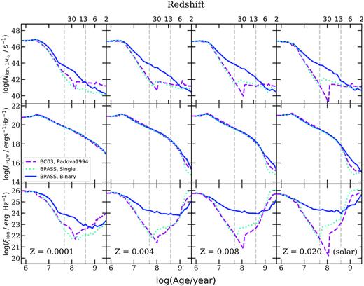
The evolution tracks of the production rate of ionizing photons per solar mass of stars formed (|$\dot{N}_{\rm ion,1\,M_\odot} $|; top row), the far-UV luminosity LFUV (also normalized to 1 M⊙; middle row), and the production efficiency of ionizing photons (ξion; bottom row) as a function of the age of a stellar population, assuming an instantaneous starburst, predicted by the BC03 (purple dashed) and bpass single (cyan dotted) and binary (blue solid) SPS models. Each column shows a different metallicity as labelled. We also show the redshifts corresponding to the age equal to the age of the Universe, which can be taken as the upper limit on the stellar population age at that redshift. The vertical grey dashed lines show the age range that is most relevant to this work, where the upper (lower) bound is marked by the median of the mass-weighted stellar age for z = 4 (z = 10) galaxy populations predicted by our model.
In this work, we convolve these SPS predictions for |$\dot{N}_\text{ion}$| with the predicted 2D histogram of stellar ages and metallicities present in each galaxy at a given output redshift. These histograms are built up as follows. At each time-step during each galaxy’s evolution, a ‘star parcel’ dm* is created with a mass determined by the H2 density in the disc and the H2-based SF recipe. Each star parcel inherits the metallicity of the cold gas in the ISM at the time it forms. Metals are deposited in the cold gas by new stars with an assumed yield, and may be removed from the ISM by stellar driven winds (see SPT15 for details). When galaxies merge, their stellar populations are combined. At an output redshift, we evaluate |$\dot{N}_\text{ion}$| for each galaxy by summing up |$\dot{N}_\text{ion}$| for each star parcel from the data tables provided by a chosen SPS model based on its stellar age and metallicity at the time.
In the previous papers in the series, we adopted the BC03 SPS models to compute the galaxy SEDs, and the model UV luminosity functions (UV LFs) have been extensively tested against existing observations. In order to avoid repeating these comparisons, we retain the estimates of LFUV based on the BC03 models in all of our results, and only compute |$\dot{N}_\text{ion}$| with the SPS model variants. Thus, the values of ξion for the bpass models are not strictly self-consistent. However, we saw in Fig. 1 that the predictions for LFUV from these two SPS models are very similar for the ages that are most relevant for our study (z ≳ 6), so this should not cause a significant discrepancy. Furthermore, ξion is only used for illustrative purposes. For actually computing the reionization history, we use |$\dot{N}_\text{ion}$| directly.
3 RESULTS
Our results are organized in three parts. (1) We compare results across different SPS models. (2) We present scaling relations and redshift evolution for ionizing photon production rates and efficiencies, and show how ξion relates to observable properties. (3) We show how variations in the SN feedback model impact our predictions for galaxies during the EoR.
3.1 Comparison across SPS models
In this subsection, we compare ξion computed with several SPS models, while other model components in our SAM remain in their fiducial configurations. As illustrated in Fig. 1, the predicted production rate of ionizing photons depends on the age and metallicity of the stellar populations, and these relations vary across different SPS models. Note that these SPS models are applied to the same galaxy populations. In other words, the galaxies used for all three SPS models have identical star formation histories and physical properties.
In Fig. 2, we show the distributions of ξion against M* for BC03 and bpass models for single and binary stellar population at selected redshifts. The 2D histograms illustrate the conditional number density per Mpc3 of galaxies in each bin and are normalized to the sum of the number density in the corresponding (vertical) stellar mass bin. The 16th, 50th, and 84th percentiles are marked in each panel to illustrate the statistical distribution. The median of predictions of all models for each given redshift are overlaid for easy comparison.
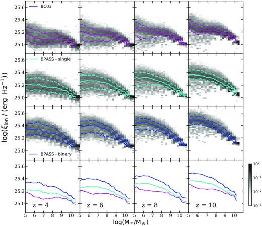
Conditional distributions of ξion versus stellar mass predicted at z = 4, 6, 8, and 10 using SPS models from BC03 (purple) and bpass (cyan and blue for single and binary). Each column shows a different redshift as labelled. The grey-scale 2D histograms show the conditional number density of galaxies in each bin, normalized to the sum of the number density per Mpc3 in each corresponding (vertical) stellar mass bin. The blue solid and dashed lines show the 50th, 16th, and 84th percentiles, respectively, for the distribution in each panel. The medians of these distributions are repeated in the bottom row for comparison, using the same colour coding as in the other panels.
In general, we see that massive galaxies have lower ξion than low-mass galaxies regardless of the choice of SPS models and redshift. Also the scatter of the relation is larger for low-mass galaxies. Although all models demonstrate some level of dependence on M*, we find that BC03 yields the weakest dependence for M* < 108 M⊙, but both bpass models predict more evolution for galaxies in the same mass range. The differences between predictions from the most and the least optimistic SPS model can be up to ∼0.2 dex for galaxies with M* ∼ 107 M⊙, and the difference shrinks for more massive galaxies.
At fixed M*, the predicted value of ξion evolves mildly as a function of redshift, with an average downward shift of ∼0.1 dex from z = 10 to z = 4. High-redshift galaxies seem to be more efficient at producing ionizing photons than their low-redshift counterparts of similar mass due to the younger stellar age and lower metallicity. We also notice the slope of the ξion-M* relation becomes more shallow with decreasing redshift, likely due to the corresponding change in the slope of the M*-Z* relation.
3.2 Comparison with numerical hydrodynamic simulations
We compare our results with predictions of ξion computed from galaxies in the bluetides simulations with various SPS models presented in W16. bluetides is a cosmological hydrodynamical simulation with 400 Mpc h−1 on a side and 2 × 70403 particles, which is able to resolve galaxies with M* ≳ 108 providing a wide variety of predictions for physical and observable properties for high-redshift galaxies up to z ∼ 8 (Feng et al. 2016; Wilkins et al. 2017). We also note that bluetides adopted a set of cosmological parameters that are consistent with constraints from WMAP9. In Fig. 3, we compare the ξion relations at z = 8 predicted by our SAM and bluetides with BC03 and bpass single and binary star models (v2.0; Stanway et al. 2016), which does not include nebular emission. The W16 calculations assumed a Salpeter (1955) IMF. We convert the quoted stellar masses to a Chabrier IMF by adding −0.21 dex for direct comparison (Madau & Dickinson 2014). The values of ξion are nearly unaffected by this change in IMF. We note that the predictions for ξion from W16 and our models are very consistent for the BC03 models, while the SAM predictions are about 0.1 dex lower for the bpass single and about 0.25 dex lower for the bpass binary models (though the qualitative trends are the same).
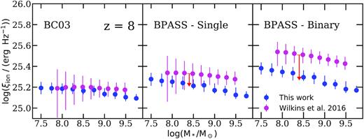
A comparison of ξion and |$\dot{N}_\text{ion}$| predicted with BC03 and bpass (both single and binary) SPS models between this work and W16. The data points mark the median and the error bars span the 16th to 84th percentile range. The red arrow shows the estimated difference in ξion changing from bpass v2.0 to v2.1 models, accounting for the metallicities difference between the SAM and bluetides galaxies, see the text for details.
In order to better understand these differences, we further compare a number of key physical properties for our model galaxies to the predictions by bluetides reported in Wilkins et al. (2017) in Fig. 4, including intrinsic (dust-free) UV mass-to-light ratio, stellar metallicity, mass-weighted stellar age, and specific star formation rate (sSFR). Note that this work assumed a Chabrier IMF, which is consistent with our work and does not require any adjustment. We also compare to the mass–metallicity relation predicted by the FIRE simulations (Hopkins et al. 2014; Ma et al. 2016a), which are high-resolution cosmological hydrodynamic zoom-in simulations. We show predictions at z = 6 in our comparison, which is the highest redshift provided in the FIRE publications. The FIRE simulations assumed a Kroupa (2001) IMF and we convert their stellar masses to a Chabrier IMF by adding −0.03 dex Madau & Dickinson (2014). It is interesting that although bluetides and FIRE have very different resolution as well as different subgrid recipes for star formation and stellar feedback, the predicted mass–metallicity relations are very similar, and much lower than the one predicted by our SAM. We discuss possible reasons for this discrepancy in Section 4, however, we do not currently have a complete understanding of this issue, and it is beyond the scope of this paper to determine.
![Comparison between the median of the intrinsic rest-UV mass-to-light ratio [$\log ((M_*/{\rm M}_\odot)/(L_{\nu , {\rm FUV}}/{\rm erg\,\,s}^{-1}\, {\rm Hz}^{-1}))$; upper left], stellar metallicity (upper right), mass-weighted stellar age (lower left), and specific SFR (lower right) for galaxies predicted by our SAM (blue) and bluetides (purple Wilkins et al. 2017). The black crosses show the stellar metallicity predicted by the FIRE simulations at z = 6 (Ma et al. 2016a). The dashed blue lines mark the 16th and 84th percentiles of the SAM predicted distributions.](https://oup.silverchair-cdn.com/oup/backfile/Content_public/Journal/mnras/494/1/10.1093_mnras_staa714/1/m_staa714fig4.jpeg?Expires=1750315161&Signature=nkUPRy6720THnsL4VH2MUQ3qA0FV8fM21numy5BAMOxqr5PQ4CwqbnpgyiLhu6GkC~xh2~s0WUhS89VuoqdUPo08XU84M0FDfi3N0wtj1UeMc8wC2gIhh3zfE7I64Sgee6l2U4sgVU6UTgoeCkYxAmvym32gO676Eujnz0dGx4aY-D4U9LipP0qTPxdw9BPYnXylbLx0h9R-IBM~Ap9hszrhBfGfNXVC7IM4~fqssvYhmSpx~llJtfGbRAs86A708vu9dc7gmIEXPlwMQ7cxrDEmP1xCa-xwvHVsN-Fm7ZBKUY2pDquwz~jCYtjBzp50J2frcCCS8YCcEMaF3uE92w__&Key-Pair-Id=APKAIE5G5CRDK6RD3PGA)
Comparison between the median of the intrinsic rest-UV mass-to-light ratio [|$\log ((M_*/{\rm M}_\odot)/(L_{\nu , {\rm FUV}}/{\rm erg\,\,s}^{-1}\, {\rm Hz}^{-1}))$|; upper left], stellar metallicity (upper right), mass-weighted stellar age (lower left), and specific SFR (lower right) for galaxies predicted by our SAM (blue) and bluetides (purple Wilkins et al. 2017). The black crosses show the stellar metallicity predicted by the FIRE simulations at z = 6 (Ma et al. 2016a). The dashed blue lines mark the 16th and 84th percentiles of the SAM predicted distributions.
The differences in the stellar population properties between the SAM and bluetides galaxies do not seem sufficient to explain the difference in the predicted value of ξion, nor it is obvious how this would explain why the differences are more pronounced for the bpass models. However, W16 used the bpass v2.0 version of the models, while we use the latest v2.2.1 version. Eldridge et al. (2017) provide a detailed discussion of the implications of changes from the v2.0 to v2.1 models for the production efficiency of ionizing photons (see their Section 6.6.1). They find that the use of improved stellar atmosphere models for low-metallicity O stars leads to a less dramatic increase in ξion from the single star to binary star case than was seen in the v2.0 models, as well as a weaker dependence of ξion on metallicity. We make use of their figure 35 to estimate the effect of changing from the v2.0 to v2.1 models, assuming the typical metallicity of the SAM and bluetides galaxies. This correction is shown by the red arrow in our Fig. 3, showing that this largely accounts for the discrepancy.
3.3 Scaling relations for the production rate and efficiency of ionizing radiation
In this subsection, we present scaling relations for ξion and |$\dot{N}_\text{ion}$| with respect to selected observable and physical properties predicted by our fiducial model configurations with the bpass binary SPS models. We also study the redshift evolution of these relations and compare to recent observations.
We show the distribution of ξion against SFR (averaged over 100 Myr), specific SFR (sSFR), intrinsic rest-frame MUV (without attenuation by dust), and cold gas metallicity (Zcold) predicted at z = 4, 6, 8, and 10 in Fig. 5. Throughout this work, we refer to the UV luminosity without a correction for attenuation effect by dust as the intrinsic MUV, which is to distinguish it from the dust-attenuated MUV. Similar to plots in previous sections, the 2D histograms indicate the conditional number density per Mpc3 of galaxies in each bin and is normalized to the sum of the number density in its corresponding (vertical) stellar mass bin. The 16th, 50th, and 84th percentiles are marked in each panel. The median of predictions made with all models for each given redshift are overlaid to illustrate the redshift evolution.
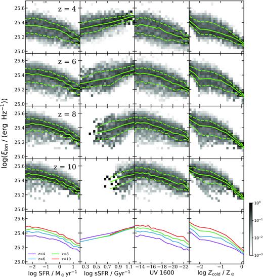
Conditional distributions of ξion versus SFR (averaged over 100 Myr), specific SFR (sSFR), intrinsic UV luminosity, and cold gas metallicity at z = 4, 6, 8, and 10 with our fiducial model configurations with the bpass binary SPS models. The green solid and dashed lines mark the 50th, 16th, and 84th percentiles. The grey-scale 2D histograms show the conditional number density of galaxies in each bin, normalized to the sum of the number density per Mpc3 in the corresponding (vertical) bin. The median of these distributions are repeated in the last row for comparison to illustrate the redshift evolution.
We find mild trends of decreasing ξion with increasing SFR, increasing ξion with increasing sSFR, decreasing ξion with increasing UV luminosity, and decreasing ξion with increasing gas-phase metallicity. The inverse trends of ξion with SFR and UV luminosity may appear counterintuitive, until we recall that both of these quantities are strongly correlated with stellar mass, and hence with metallicity, so the inverse correlation between metallicity and ξion is likely driving this result. As seen in Fig. 4, there is only a weak trend between stellar mass and mean stellar age in our models. At fixed SFR, UV luminosity, and cold gas metallicity, ξion decreases with cosmic time from z ∼ 10 to 4, due to the increasing fraction of relatively old stars. Only for fixed sSFR is ξion nearly constant with redshift, indicating that this quantity is correlated with the fraction of young stars.
Fig. 6 shows the distribution of ξion, predicted for halo populations between z = 4–10. We see that for haloes of the same mass, the production efficiency of ionizing photons can change by up to ∼0.2 dex between z = 10 and 4. Similarly, Fig. 7 shows the distribution of the specific ionizing photon production rate, |$\dot{N}_\text{ion}/M_\text{h}$|, predicted for the same set of haloes, where the production rate of ionizing photons can be up to ∼1.5 orders of magnitude higher at z = 10 relative to z = 4 for haloes of the same mass. This relation evolves much more rapidly than the stellar-to-halo mass ratio (SHMR) presented in Paper II. This is due to our finding (presented in Paper II) that galaxies at high redshift are intrinsically brighter in the UV than their low-redshift counterparts of similar stellar mass due to the higher SFR, younger stellar population, and lower metallicities.
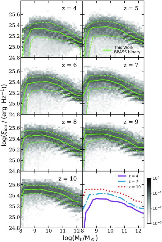
Predicted ξion as a function of halo mass between z = 4–10 predicted with the bpass binary model. The green solid and dashed lines mark the 50th, 16th, and 84th percentiles. The 2D histograms are colour-coded to show the conditional number density per Mpc3 of galaxies in each bin, normalized to the sum of the number density in the corresponding (vertical) halo mass bin. The last panel show an overlay of the SHMR median predicted at z = 4, 7, and 10 from our model.
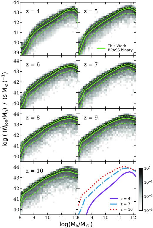
Specific ionizing photon production rate, |$\dot{N}_\text{ion}/M_\text{h}$|, as a function of halo mass between z = 4–10 predicted with the bpass binary model. The green solid and dashed lines mark the 50th, 16th, and 84th percentiles. The grey-scale 2D histograms show the conditional number density per Mpc3 of galaxies in each bin, normalized to the sum of the number density in the corresponding (vertical) halo mass bin. The last panel shows the median |$\dot{N}_\text{ion}/M_\text{h}$| relations predicted at z = 4, 7, and 10 from our model.
On the other hand, ξion does not evolve as much across redshift since both |$\dot{N}_\text{ion}$| and LFUV evolve in the same direction. In Fig. 8, we illustrate the evolution of ξion as a function of redshift. We show predictions from our fiducial model with both bpass and BC03 SPS models at the bracketing UV magnitudes of MUV = −22 and −17 and compare these to a compilation of observational estimates. Both our predictions and the observations are colour-coded for rest-frame MUV. These measurements are derived from H α flux and UV-continuum luminosity (Bouwens et al. 2016a; Rasappu et al. 2016; Smit et al. 2016; Lam et al. 2019), H α flux and UV-based SFR (Shim et al. 2011; Mármol-Queraltó et al. 2016), C iv measurement (Stark et al. 2015), and SED fitting (Stark et al. 2017). We indicate the range of log ξion = 24.0–25.7 derived from ∼14 000 compact star-forming galaxies found in the Sloan Digital Sky Survey (SDSS; DR12) between 0 < z < 1 for comparison (Izotov et al. 2017). We also include the luminosity-weighted ξion from W16 at =8–10. We compare our predictions to the results from the FirstLight simulations, which is a set of high-resolution zoom-in simulations based on cosmological boxes of 10, 20, and 40 Mpc h−1 on a side, resolving galaxies in haloes with circular velocities spanning the range between 50 and 250 km s−1 at z ≳ 5 (Ceverino, Glover & Klessen 2017; Ceverino et al. 2019). The computation for ξion is based on synthetic SEDs from bpass (v2.1, Eldridge et al. 2017) including nebular emission (Xiao, Stanway & Eldridge 2018) and a Kroupa-like IMF. Note that whilst the simulations have been run with both WMAP and Planck cosmologies, the results referenced here are only available with the WMAP5 cosmology. For reference, we also label the range of typical values ξion ≈ 25.20–25.30 that are assumed in many analytic studies (e.g. Bouwens et al. 2012; Finkelstein et al. 2012; Kuhlen & Faucher-Giguère 2012; Duncan & Conselice 2015; Robertson et al. 2015). Our models predict very mild evolution in ξion as a function of redshift and a very consistent ∼0.1–0.15 dex difference between the bright (MUV = −22) and faint (MUV = −17) galaxies. The red arrow shows an estimate (from fig. 35 of Eldridge et al. 2017) of the increase in ξion if the upper mass limit of the IMF were changed from 100 to 300 M⊙, illustrating how sensitive ξion is to the upper end of the stellar IMF. In addition, lower redshift measurements reporting ξion ≳ 25.5 at z ∼ 3 appear to be in tension with standard model assumptions (Nakajima et al. 2016, 2018). We also note that estimates of ξion from detected rest-UV emission lines at higher redshifts (e.g. z > 5) tend to be obtained for sources with detectable nebular lines. As there is a general correlation between the equivalent width (EW) in these lines and ξion, the published ξion values based on rest-UV lines are likely biased towards the upper end of the true range of values, rather than reflecting the mean or median of the overall population at these epochs.
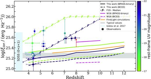
A comparison of the redshift evolution of ξion predicted by our models to a compilation of observations and empirical constraints. The solid and dashed lines denote our predictions using BC03 (solid) and the bpass binary SPS (dashed) models and are colour-coded for rest-frame dust-attenuated MUV. Here, we show the two bracketing cases representing bright (MUV = −22) and faint (MUV ∼ = − 17) galaxies shown in dark blue and green, respectively. The red arrow shows an estimate of the increase in ξion if the upper mass limit of the IMF were changed from 100 to 300 M⊙. We also plot the median parameters obtained by F19 for the same bracketing MUV, shown with a dotted line with a ‘F’ marker. The solid and dashed purple lines show the luminosity-weighted value of ξion for galaxies with M* > 108 M⊙ at z = 8–10 predicted by W16 with the SPS models considered in this work. The solid orange line shows results from the FirstLight simulations, which assumed a bpass binary SPS model (Ceverino et al. 2019). We include a compilation of observations from Shim et al. (2011), Stark et al. (2015, 2017), Bouwens et al. (2016a), Smit et al. (2016), Rasappu et al. (2016), Lam et al. (2019) for comparison; see the text for a description. All observations and model predictions are colour-coded for rest-frame UV magnitude. Typical values adopted in analytic calculations are highlighted by the grey band. We also show the range derived from a large sample of SDSS galaxies at 0 < z < 1 (Izotov et al. 2017). The lower bound of this range extends to ξion = 24 (not shown).
F19 obtained indirect constraints on the plausible range of ξion using an empirical model. They parametrization ξion as a function of redshift and rest-frame MUV, and obtained the posterior on these parameters (along with other model parameters) using Markov chain Monte Carlo (MCMC). They found that it was possible to satisfy constraints on the reionization history of the Universe with a relatively low average escape fraction (of about 5 per cent) if ξion is higher in lower luminosity and higher redshift galaxies. The median posterior parameters found in their analysis are dlog ξion/dz = 0.13 and dlog ξion/dz = 0.08, and a reference magnitude of MUV,ref = 20. Although our models predict these qualitative trends, our predicted trends are not nearly as strong as the ones suggested by the F19 models. We will investigate resolutions to this tension in more detail in Paper IV of this series.
Next we attempt to make predictions for correlations between physical and observable galaxy properties and ξion in order to suggest strategies for future observations. In Fig. 9, we show observed-frame magnitude in the NIRCam F200W filter, mF200W, versus the UV-continuum slope, βUV, in the xy-plane and colour code each cell by ξion. The detection limits for JWST wide- and deep-field observations are also marked for quick reference, which are obtained assuming survey configurations that are comparable to those of past HST surveys and the published NIRCam sensitivities with the F200W filter (see Paper I). We present these predictions for z = 4, 5, and 6, where many galaxies should be bright enough that spectra will be relatively efficiently obtained with JWST or other facilities. We show a similar plot for sSFR and stellar metallicity in Fig. 10.
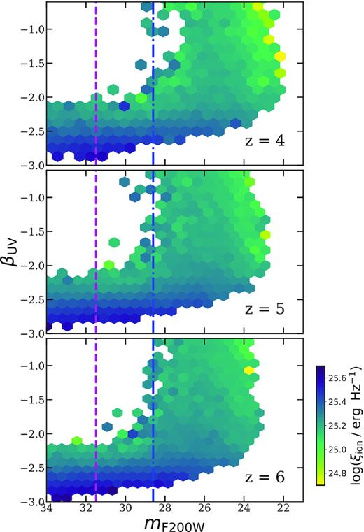
Correlation of βUV and mF200W at z = 4, 5, and 6 in our fiducial models, with the average value of ξion in each hexbin colour-coded. The vertical lines mark the detection limit of a typical JWST NIRCam wide and deep surveys at mF200W,lim = 28.6 and 31.5, respectively. The left edges of these plots coincide with the detection limit for lensed surveys.

Correlation of stellar metallicity and SFR at z = 4, 5, and 6 in our fiducial models, with the average value of ξion in each hexbin colour-coded.
3.4 The impact of SN feedback
As shown in previous works in this series, the number density of faint, low-mass galaxies is very sensitive to the feedback strength, as stronger feedback suppresses star formation by ejecting gas from the ISM. However, the faint- and low-mass-end slope of UV LFs and SMF at high redshift are not well constrained by current observations. In Paper I and Paper II, we experimented with alternative SN feedback slopes αrh, which effectively characterize the dependence of mass outflow rate on circular velocity, and found that a fiducial value of αrh = 2.8 yielded predictions that best match existing observational constraints. We further found that a range of values from αrh = 2.0 (weaker feedback) to αrh = 3.6 (stronger feedback) yielded predictions that are well within the current observational uncertainties. In this subsection, we explore how varying this model parameter impacts the production of ionizing photons.
Fig. 11 presents the fractional difference of the median of the predicted |$\dot{N}_\text{ion}$| between our fiducial model (αrh = 2.8) and model variances with stronger (αrh = 3.6) and weaker (αrh = 2.0) SN feedback, computed using a sliding boxcar filter of width |$\Delta {\rm log} (M_* / \mathrm{ M}_\odot) = 1.0$| in stellar mass. We find that the range of αrh that yields galaxy populations within the observational uncertainties may cause |$\sim 20{{\ \rm per\ cent}}$| differences in |$\dot{N}_\text{ion}$|, where more ionizing photons are produced when feedback is stronger and vice versa. This is likely caused by the more bursty star formation in the presence of stronger feedback. Although stronger feedback may boost the production efficiency of ionizing photons for low-mass galaxies, we must keep in mind that stronger feedback also suppresses the formation of low-mass galaxies, leading to lower overall UV luminosity density, so there is a trade-off. We show in Fig. 12 and in our forthcoming Paper IV that in our models, stronger feedback leads to an overall decrease in the total number of ionizing photons. However, different implementations of stellar feedback could in principle produce different results.
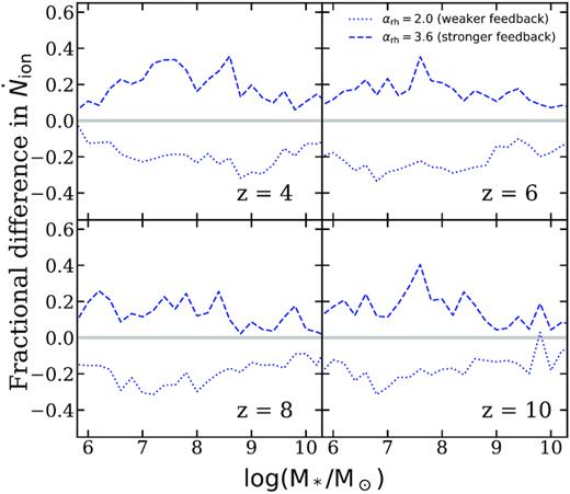
The fractional difference of the median of the distribution of ξion versus stellar mass for different SN feedback slopes predicted at z = 4, 6, 8, and 10 with other model parameters and ingredients left at their fiducial values. The dashed and dotted blue lines represent the stronger and weaker feedback scenarios.
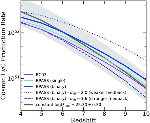
Cosmic LyC photon production rate evolution with redshift given in units of Mpc−3 s−1, calculated using SPS models from BC03 (purple) and bpass (cyan and blue for single and binary). For different SN feedback slopes predicted at z = 4–10 with other model parameters and ingredients left at their fiducial values, the dashed and dotted blue lines represent the stronger and weaker feedback scenarios, respectively. The grey lines show the case where log (ξion) = 25.30 ± 0.30.
4 DISCUSSION
In this work, we compute the production rate |$\dot{N}_\text{ion}$| and production efficiency ξion of ionizing photons by combining SPS models with a physically grounded model of galaxy formation set in a cosmological framework, the Santa Cruz SAM. Our fiducial model incorporates multiphase gas partitioning and H2-based star formation recipes (GK-Big 2), which have been shown to reproduce observational constraints over a wide range of redshifts from z = 0–10 (see PST14, SPT15, Paper I, and Paper II). |$\dot{N}_\text{ion}$| and ξion for composite stellar populations depends on the joint distribution of ages and metallicities in each galaxy. These quantities may in principle evolve with redshift or be correlated with global galaxy properties such as mass or luminosity. It is thus important to use a self-consistent, physically grounded model that hopefully contains the relevant internal correlations between physical properties. This is a significant advantage of our approach.
We compare |$\dot{N}_\text{ion}$| and ξion calculated using different SPS models, which depends on the physical properties of the stellar populations, such as star formation and metal enrichment histories. This approach of modelling |$\dot{N}_\text{ion}$| also makes physical predictions for the correlations among ξion and |$\dot{N}_\text{ion}$| with other physical properties, such as M*, Z*, SFR, etc., and observable properties, such as βUV and observed frame magnitude. We also take advantage of the high efficiency of our model to explore how these predictions may be impacted by modelling uncertainties regarding SN feedback.
4.1 Comparison with observations
Our predictions for ξion are in good agreement with most of the observational measurements at 4 < z < 5, but despite the range of models we investigated in this work, none of our models reproduce the observed values of ξion at z > 5. Our models tend to predict values of ξion at z ∼ 7 that are lower than the observational estimates by about 0.3 dex. Here, we briefly discuss a few reasons that could give rise to this discrepancy. First, inferring ξion from observations is highly non-trivial. This estimate relies on obtaining the intrinsic rest-frame MUV using the UV slope βUV to correct for dust extinction. However, it is not known how reliable the empirical relations between UV slope and attenuation are at these redshifts, and uncertainties in the underlying shape of the attenuation curve also lead to uncertainties (Bouwens et al. 2016a).
In addition, due to limitations in current survey instruments, objects with extremely bright emission lines are preferentially selected for follow-up. These may be biased towards objects at the extreme tails of the distribution of physical properties, or towards rare starbursting galaxies. The large sample of lower redshift galaxies (0 < z < 1) studied by Izotov et al. (2017) show a broad range of values of ξion, and suggest the strong sensitivity in this parameter to recent bursts.
Finally, the estimates of ξion from the SPS models are still quite uncertain. For example, the predicted values of ξion dropped by about 0.1 to 0.2 dex following changes to the stellar atmosphere models implemented in v2.1 of the bpass models. However, Eldridge et al. (2017) note that an improved treatment of rotation could increase ξion by a similar amount (see also Levesque et al. 2012). Furthermore, ξion is quite sensitive to the high-mass end of the stellar IMF. For example, Eldridge et al. (2017) show that increasing the upper mass cut-off of the IMF from 100 to 300 M⊙ increases the value of ξion by about 0.15 dex in the v2.1 bpass binary models.
4.2 Our results in the context of other theoretical studies
SAMs and hydrodynamic simulations are two different approaches to modelling galaxy formation (see Somerville & Davé 2015 for a detailed discussion), but they both require the use of phenomenological recipes for processes that cannot be explicitly simulated, such as star formation and stellar feedback. Both our models and the bluetides simulations adopted similar multiphase gas partitioning and H2-based star formation recipes, however, a number of other differences in the models may contribute to the discrepancies in their predictions. These include the choice of IMF, the quantities given priority in the calibration process, and the set of cosmological parameters adopted. bluetides adopts cosmological parameters that are consistent with measured values reported by WMAP, which are different from the ones adopted in this work. However, we do not expect this to lead to major differences in the relevant predicted galaxy properties (see discussion in Appendix C in Paper II). In the model comparison presented in Paper I and Paper II, we showed that the predicted statistical properties (rest-UV LFs, stellar mass functions, SFR functions) of galaxies at z ∼ 8–10 are nearly identical in our models and in bluetides. However, when we compared our predicted values of ξion at a given stellar mass at z ∼ 8 with those predicted by W16 for bluetides, we find that the values agree well for the BC03 SPS models, while our predicted values are lower by about 0.1 dex for the single star bpass models and about 0.2 dex lower for the bpass models that include binary star evolution. We argue, based on the results presented in Eldridge et al. (2017), that this difference is largely accounted for by changes in the bpass model results from the v2.0 version used by W16 to the v2.2.1 version that we have adopted in this work. This is supported by the fact that the predicted value of ξion from the FirstLight simulations (which also adopted the bpass v2.2.1 models) are quite similar to ours.
When we compare the other stellar population properties of galaxies in bluetides and our models at the same stellar mass and redshift (z = 8), we find that our galaxies are slightly younger and have higher sSFRs. By far the most significant difference, however, is that the stellar populations have mass-weighted metallicities that are a factor of 6 higher in our models than in bluetides.
All of the physically grounded models in the literature (including bluetides, FirstLight, and our models) predict rather mild redshift evolution in ξion as well as generally lower values than those implied by observations at z ≳ 5.
4.3 Caveats and limitations of the modelling framework
The productivity of ionizing photons of high-redshift galaxies connects the small-scale processes of stellar evolution, star formation, and stellar feedback with cosmological scale processes such as the reionization of intergalactic hydrogen. Our results depend critically on SPS models, which have their own limitations and uncertainties (Conroy 2013). The massive, low-metallicity stars that are the most efficient at producing ionizing photons are particularly sensitive to modelling uncertainties in physical processes, such as mass-loss, mixing, convection, rotation, and magnetic fields; and significant progress has been made in the past few years on improving these models. One area that has received some attention within the literature on high-redshift galaxy populations and the EoR recently is the impact of binary processes on the evolution of massive stars and the implications for the production of ionizing photons (Ma et al. 2016a; Wilkins et al. 2016; Ceverino et al. 2019). Binarity can have a significant effect on the production rate of ionizing photons via a diverse range of physical mechanisms. Mass transfer and mergers among binaries can increase the number of massive stars present over times longer than the lifetime of massive single stars. In addition, mass transfer can produce rapidly rotating ‘chemically homogeneous’ stars, which are more prevalent at low metallicity and are highly efficient at producing ionizing photons. The rotating massive stellar population can be an significant source of ionizing photons in the first ∼4 Myr for starburst galaxies (Choi, Conroy & Byler 2017). A third process is that stars in a binary system can be stripped of their envelope, exposing the hot core of the star. Stripped stars can boost the production rate of ionizing photons at times 20–500 Myr after the onset of star formation by as much as 1–2 orders of magnitude Götberg et al. (2019). The bpass models adopted in this work include modelling of these processes (Eldridge, Langer & Tout 2011; Eldridge & Stanway 2012; Stanway et al. 2016; Eldridge et al. 2017), while the role of stripped stars has been highlighted in Götberg et al. (2019). Other processes that may be important for producing ionizing photons, but which are not accounted for or not modelled in as much detail in the bpass models, include accreting white dwarfs and X-ray binaries (Madau & Fragos 2017). Because ξion is so sensitive to the most massive stars, it is also quite sensitive to details of the high-mass slope and cut-off of the stellar IMF (e.g. Eldridge et al. 2017). In summary, the raw predictions of ξion even in the latest models seem to be uncertain at the level of at least a factor of 2.
Moving up in scale, the star formation and chemical enrichment histories that form the backbone of this work are based on the modelling framework developed in a series of papers including SPT15, Paper I, and Paper II. These models make a large number of simplifying assumptions about how baryonic processes in galaxies operate. A fundamental ansatz of our models is that the scaling relations that describe processes such as gas partitioning, star formation efficiency, and stellar feedback are valid over all of cosmic time. This may not necessarily be the case. Our adopted scaling relations may have dependencies that do not properly track the true physical properties, which may evolve differently. These assumptions are typically tested and calibrated by comparing with observations. As shown in these previous works, the predicted distribution functions for MUV, M*, and SFR up to z ∼ 10 are in very good agreement with observations in regimes where observational constraints are available. However, the physical properties of high-redshift faint galaxies, as well as the underlying physical processes that drive them, are poorly constrained.
The results of this work hint that the treatment of stellar feedback and chemical evolution may be an area that requires careful examination in future work. Although our models produce excellent agreement with both the bluetides and FIRE simulations with regard to bulk properties such as the SHMR, as noted above, the predicted mass–metallicity relation at z ∼ 6–8 is substantially different. As shown in fig. 7 of Ma et al. (2016b) and fig. 6 of Somerville & Davé (2015), the predicted mass–metallicity relation shows a large dispersion between different models and simulations. This is because there are many details of the chemical enrichment process that are poorly understood or simplified in cosmological galaxy formation models. For example, the version of the SC-SAM models used here assumes instantaneous recycling, i.e. that metals ejected by SNe are instantaneously mixed with the whole ISM. Our models assume a fixed chemical yield, y, which is treated as a fixed parameter that is tuned such that the predicted stellar mass–metallicity relation matches z ∼ 0 observations. We also assume that the metallicity of outflows is the same as that of the ISM, while there is evidence in nearby galaxies that stellar driven winds may be substantially metal-enhanced (metals preferentially ejected Chisholm, Tremonti & Leitherer 2018). Furthermore, we note that the multiphase gas partitioning recipes adopted in our models may break down in extremely metal-poor environments (Sternberg et al. 2014). Neither primordial H2 cooling and Pop III stars nor metal enrichment by these objects is explicitly included in our models. Instead, top-level progenitor haloes are polluted to a metallicity floor with typical values of Zpre-enrich = 10−3 Z⊙.
4.4 Characterizing ionizing sources with JWST and beyond
As shown in Fig. 9, predictions from our model show that βUV may not be an very good tracer for ξion as the correlation between quantities is rather weak. The productivity of ionizing photons can be indirectly traced with a number of spectral features. Due to current instrumental limitations, it is tremendously challenging to obtain high-resolution spectra for galaxies at high redshifts. The NIRSpec onboard JWST possesses the advanced capability for detecting Hα at z ≲ 7, and given adequate exposure time, the mid-infrared instrument will also be able to pick up signals from bright objects at z ≳ 7. Furthermore, planned flagship ground-based telescopes, such as the ELT, the Thirty Meter Telescope, and the Giant Magellan Telescope, are also expected to enable these kinds of observations for many more objects and for fainter, perhaps more ‘typical’ galaxies. These anticipated observations will be able to constrain or even rule out completely some of the predictions provided in this work.
4.5 Implications of our results for cosmic reionization
A summary of our predictions for the intrinsic cosmic ionizing emissivity is shown in Fig. 12. This figure illustrates the impact of adopting different stellar population models (self-consistently incorporated within our models) and of varying the strength of stellar feedback. As discussed above, the rather strong metallicity dependence of ξion implies that the details of the interplay between chemical evolution and stellar populations can lead to differences of up to factors of a few, which could be significant for reionization. The total number of ionizing photons produced are degenerately affected by the abundance of galaxies during the EoR and the intrinsic productivity of ionizing radiation. As shown in Paper I and Paper II, the abundances of low-mass galaxies are very sensitive to the strength of SN feedback and the number of objects predicted can span about an order of magnitude for different model assumptions. On the other hand, in Section 3.4 we also show that stronger feedback yields slightly (|$\sim 20{{\ \rm per\ cent}}$|) boosted ionizing photon production efficiencies.
Whether galaxies alone are sufficient to ionize the IGM remains a fundamental open question. Historically, there has been tension between the total ionizing photon budget accounted for by galaxies, and constraints on the onset and duration of the EoR. Analytic calculations (e.g. Kuhlen & Faucher-Giguère 2012; Robertson et al. 2015) have shown that galaxies are likely to have produced sufficient numbers of ionizing photons to reionize the Universe under the condition that faint objects remain fairly numerous below the current detection limit and are fairly efficient at producing ionizing photons. In Paper I and Paper II, we showed that in our models, the faint-end slope of the rest-frame UV LF remains steep down to MUV ∼ −9, under the assumption that SNe feedback at high redshifts operates with similar efficiency as that required to match z ∼ 0 observations. The predicted ionizing photon production efficiencies, especially with models that include binary evolution, are well within the range log (ξion) ∼ 25.30 ± 0.30 (or higher) adopted in recent models that are able to plausibly account for observable constraints on the reionization history (Kuhlen & Faucher-Giguère 2012; Robertson et al. 2013, 2015; Finkelstein et al. 2019). Therefore, we can already anticipate that our models will also produce good agreement with the observed reionization history, subject to uncertainties on the escape fraction of ionizing radiation. We present a detailed analysis of the implications for the cosmic reionization history of our full modelling framework, including the escape fraction, in Paper IV.
5 SUMMARY AND CONCLUSIONS
In this work, we implemented a physically motivated approach to calculating |$\dot{N}_\text{ion}$| in the Santa Cruz SAM, accounting for stellar age and metallicity distribution of the stellar population in each galaxy. We present results predicted based on SSP models from BC03 and both single and binary stellar population by bpass. Taking advantage of the high efficiency of our modelling framework, we make predictions for galaxies across z = 4–10, forming in a wide range of halo masses, ranging from Vvir ≈ 20–500 km s−1. These predictions provide forecasts for future observations with JWST and also put modelling constraints on the role high-redshift, low-mass galaxies played throughout the EoR. We also provide predicted scaling relations of |$\dot{N}_\text{ion}$| with M*, Mh, βUV, and other galaxy properties. We compared our predictions to other models from the literature and the latest observations in both the intermediate- and high-redshift universe.
We summarize our main conclusions below.
In agreement with previous work, we find that SPS models accounting for binary stellar populations can produce a factor of ∼2 more ionizing radiations than models that only account for single star populations for galaxies across all mass ranges.
We find that faint, low-mass galaxies can have ionizing efficiencies that are up to a factor of 2 higher than those of bright, massive ones. This is due to the strong correlation between stellar mass (or luminosity) and metallicity that is already in place at early times in our models, and the strong dependence of ξion on metallicity, particularly in models that include physical processes related to stellar binaries.
Our models predict a rather weak dependence of ξion with redshift (about ∼0.23 dex or factor of ∼0.6 decrease from z ∼ 12 to 4).
We find that increasing of the strength of SN feedback may allow galaxies to produce |$\sim 20{{\ \rm per\ cent}}$| more ionizing photons, because their star formation is more bursty. However, we also note that stronger feedback suppresses star formation in low-mass haloes and decreases the number density of low-mass galaxies, which ultimately decreases the total number of ionizing photons.
Our predicted median values of ξion are significantly lower than all current observational estimates at z > 5. This may be due to sampling bias towards extremely bright and bursty objects in current high-redshift observations, or to modelling uncertainties in SPS models.
We provide scaling relations for |$\dot{N}_{\rm{ion}}$| as a function of Mh and a number of other galaxy properties, which may be useful for cosmological scale reionization simulations where baryonic physics is not resolved.
ACKNOWLEDGEMENTS
The authors of this paper would like to thank Adriano Fontana et al. for organizing the ‘The Growth of Galaxies in the Early Universe – V’ conference in Sesto, Italy, which fostered significant discussions that inspired the creation of this work. We also thank Selma de Mink and Stephen Wilkins for useful comments and discussions. We also thank the anonymous referee for the constructive comments that improved this work. AY and RSS thank the Downsbrough family for their generous support, and gratefully acknowledge funding from the Simons Foundation.
Footnotes
https://bpass.auckland.ac.nz/, v2.2.1
REFERENCES
APPENDIX A: TABULATED VALUES FOR IONIZING PHOTON PRODUCTIVITY
Tabulated |$\log (\dot{N}_\text{ion}/M_\text{h})$| from our fiducial model is provided in Table A1. Other scaling relations shown in this work are available online.
Tabulated |$\log (\dot{N}_\text{ion}/M_\text{h})$| at z = 4–10 from our fiducial model. These are the median values as shown in Fig. 7. The upper and lower limits represent the value of the 84th and the 16th percentile.
| |$\log _{10}((\dot{N}_\text{ion}/M_\text{h})\,\, /\,\, (\mathrm{ s}\,\mathrm{ M}_\odot)^{-1})$| | |||||||
|---|---|---|---|---|---|---|---|
| |$\log _{10}(M_{\rm h}/ \rm M_\odot )$| | z = 4 | z = 5 | z = 6 | z = 7 | z = 8 | z = 9 | z = 10 |
| 8.25 | 39.17|$^{+0.47}_{-0.70}$| | 39.62|$^{+0.54}_{-0.66}$| | 40.04|$^{+0.57}_{-0.65}$| | 40.46|$^{+0.52}_{-0.66}$| | 41.07|$^{+0.40}_{-0.72}$| | 41.29|$^{+0.31}_{-0.60}$| | 41.45|$^{+0.24}_{-0.54}$| |
| 8.50 | 39.68|$^{+0.42}_{-0.66}$| | 40.48|$^{+0.42}_{-0.79}$| | 40.93|$^{+0.31}_{-0.66}$| | 41.21|$^{+0.26}_{-0.47}$| | 41.34|$^{+0.31}_{-0.45}$| | 41.55|$^{+0.25}_{-0.55}$| | 41.68|$^{+0.23}_{-0.53}$| |
| 8.75 | 40.46|$^{+0.32}_{-0.72}$| | 40.94|$^{+0.28}_{-0.60}$| | 41.22|$^{+0.30}_{-0.50}$| | 41.41|$^{+0.31}_{-0.45}$| | 41.64|$^{+0.27}_{-0.48}$| | 41.77|$^{+0.27}_{-0.54}$| | 41.89|$^{+0.25}_{-0.60}$| |
| 9.00 | 40.88|$^{+0.30}_{-0.66}$| | 41.22|$^{+0.32}_{-0.59}$| | 41.45|$^{+0.31}_{-0.47}$| | 41.68|$^{+0.28}_{-0.49}$| | 41.85|$^{+0.27}_{-0.46}$| | 42.02|$^{+0.25}_{-0.57}$| | 42.12|$^{+0.26}_{-0.60}$| |
| 9.25 | 41.21|$^{+0.33}_{-0.61}$| | 41.48|$^{+0.31}_{-0.50}$| | 41.72|$^{+0.33}_{-0.45}$| | 41.92|$^{+0.28}_{-0.43}$| | 42.10|$^{+0.27}_{-0.55}$| | 42.27|$^{+0.23}_{-0.49}$| | 42.38|$^{+0.21}_{-0.66}$| |
| 9.50 | 41.45|$^{+0.33}_{-0.54}$| | 41.72|$^{+0.33}_{-0.46}$| | 41.97|$^{+0.28}_{-0.44}$| | 42.16|$^{+0.28}_{-0.51}$| | 42.31|$^{+0.26}_{-0.55}$| | 42.47|$^{+0.23}_{-0.56}$| | 42.61|$^{+0.20}_{-0.55}$| |
| 9.75 | 41.68|$^{+0.39}_{-0.47}$| | 41.97|$^{+0.34}_{-0.46}$| | 42.20|$^{+0.28}_{-0.45}$| | 42.36|$^{+0.26}_{-0.40}$| | 42.57|$^{+0.20}_{-0.44}$| | 42.72|$^{+0.15}_{-0.44}$| | 42.83|$^{+0.16}_{-0.52}$| |
| 10.00 | 41.89|$^{+0.36}_{-0.47}$| | 42.18|$^{+0.30}_{-0.39}$| | 42.42|$^{+0.25}_{-0.38}$| | 42.60|$^{+0.22}_{-0.42}$| | 42.77|$^{+0.18}_{-0.35}$| | 42.88|$^{+0.17}_{-0.39}$| | 43.01|$^{+0.13}_{-0.50}$| |
| 10.25 | 42.09|$^{+0.37}_{-0.45}$| | 42.38|$^{+0.29}_{-0.38}$| | 42.60|$^{+0.25}_{-0.32}$| | 42.78|$^{+0.21}_{-0.36}$| | 42.95|$^{+0.16}_{-0.40}$| | 43.05|$^{+0.16}_{-0.42}$| | 43.16|$^{+0.17}_{-0.43}$| |
| 10.50 | 42.32|$^{+0.31}_{-0.40}$| | 42.60|$^{+0.24}_{-0.36}$| | 42.82|$^{+0.21}_{-0.35}$| | 42.98|$^{+0.18}_{-0.31}$| | 43.14|$^{+0.16}_{-0.38}$| | 43.22|$^{+0.17}_{-0.37}$| | 43.28|$^{+0.20}_{-0.43}$| |
| 10.75 | 42.54|$^{+0.29}_{-0.44}$| | 42.79|$^{+0.24}_{-0.37}$| | 43.06|$^{+0.17}_{-0.42}$| | 43.15|$^{+0.17}_{-0.39}$| | 43.28|$^{+0.17}_{-0.43}$| | 43.36|$^{+0.17}_{-0.45}$| | 43.42|$^{+0.20}_{-0.47}$| |
| 11.00 | 42.81|$^{+0.22}_{-0.49}$| | 43.06|$^{+0.15}_{-0.47}$| | 43.23|$^{+0.13}_{-0.39}$| | 43.34|$^{+0.13}_{-0.41}$| | 43.44|$^{+0.16}_{-0.43}$| | 43.47|$^{+0.19}_{-0.41}$| | 43.55|$^{+0.20}_{-0.54}$| |
| 11.25 | 43.04|$^{+0.14}_{-0.57}$| | 43.22|$^{+0.13}_{-0.43}$| | 43.35|$^{+0.13}_{-0.46}$| | 43.47|$^{+0.14}_{-0.41}$| | 43.47|$^{+0.21}_{-0.40}$| | 43.55|$^{+0.22}_{-0.48}$| | 43.61|$^{+0.21}_{-0.50}$| |
| 11.50 | 43.18|$^{+0.10}_{-0.50}$| | 43.34|$^{+0.14}_{-0.44}$| | 43.43|$^{+0.15}_{-0.39}$| | 43.51|$^{+0.17}_{-0.38}$| | 43.59|$^{+0.19}_{-0.45}$| | 43.61|$^{+0.22}_{-0.46}$| | 43.60|$^{+0.28}_{-0.54}$| |
| 11.75 | 43.23|$^{+0.15}_{-0.45}$| | 43.37|$^{+0.15}_{-0.47}$| | 43.44|$^{+0.17}_{-0.33}$| | 43.52|$^{+0.17}_{-0.33}$| | 43.54|$^{+0.20}_{-0.41}$| | 43.54|$^{+0.23}_{-0.42}$| | 43.53|$^{+0.25}_{-0.47}$| |
| 12.00 | 43.13|$^{+0.26}_{-0.60}$| | 43.24|$^{+0.21}_{-0.36}$| | 43.31|$^{+0.20}_{-0.30}$| | 43.38|$^{+0.19}_{-0.37}$| | 43.42|$^{+0.20}_{-0.34}$| | 43.46|$^{+0.21}_{-0.36}$| | 43.40|$^{+0.29}_{-0.44}$| |
| 12.25 | 42.80|$^{+0.28}_{-1.11}$| | 43.00|$^{+0.18}_{-0.28}$| | 43.12|$^{+0.21}_{-0.31}$| | 43.22|$^{+0.23}_{-0.32}$| | 43.33|$^{+0.18}_{-0.34}$| | 43.38|$^{+0.21}_{-0.43}$| | 43.34|$^{+0.24}_{-0.33}$| |
