-
PDF
- Split View
-
Views
-
Cite
Cite
Philip Chang, Shane W Davis, Yan-Fei Jiang(姜燕飞), Time-dependent radiation hydrodynamics on a moving mesh, Monthly Notices of the Royal Astronomical Society, Volume 493, Issue 4, April 2020, Pages 5397–5407, https://doi.org/10.1093/mnras/staa573
Close - Share Icon Share
ABSTRACT
We describe the structure and implementation of a radiation hydrodynamic solver for manga, the moving-mesh hydrodynamics module of the large-scale parallel code, Charm N-body GrAvity solver (changa). We solve the equations of time-dependent radiative transfer (RT) using a reduced speed of light approximation following the algorithm of Jiang et al. By writing the RT equations as a generalized conservation equation, we solve the transport part of these equations on an unstructured Voronoi mesh. We then solve the source part of the RT equations following Jiang et al. using an implicit solver, and couple this to the hydrodynamic equations. The use of an implicit solver ensures reliable convergence and preserves the conservation properties of these equations even in situations where the source terms are stiff due to the small coupling time-scales between radiation and matter. We present the results of a limited number of test cases (energy conservation, momentum conservation, dynamic diffusion, linear waves, crossing beams, and multiple shadows) to show convergence with analytic results and numerical stability. We also show that it produces qualitatively the correct results in the presence of multiple sources in the optically thin case.
1 INTRODUCTION
Smooth particle hydrodynamics (SPH) is based upon the Lagrangian view of the Euler equations where the sampling of a fluid is determined from a finite number of particles, and fluid quantities like density and pressure are determined by computing a smoothing kernel over a number of neighbous. The Lagrangian nature of SPH allows it to conserve linear and angular momentum, but comes at the expense of comparatively poor resolution of shocks due to its smoothing nature. On the other hand, grid-based methods have superior shock capturing abilities due to the use of Godonov schemes, but suffer from grid effects, e.g. the presence of grid direction can affect the conservation of linear and angular momentum.
Springel (2010, hereafter S10) developed an arbitrary Lagrangian–Eulerian or moving-mesh (MM) scheme in an effort to capture the best characteristics of both approaches. S10’s scheme relies on a Voronoi tessellation to generate well-defined and unique meshes for an arbitrary distribution of points, which deform continuously under the movement of the mesh-generating points. Implemented into the code, arepo, it has been used to study a number of different astrophysical problems including cosmological galaxy formation (see, e.g. Vogelsberger et al. 2014), discs, and stellar mergers (Zhu et al. 2015; Ohlmann et al. 2016).
Aside from arepo, a number of MM codes have been developed based on S10’s scheme. These include tess (Duffell & MacFadyen 2011), fvmhd3d (Gaburov, Johansen & Levin 2012), shadowfax (Vandenbroucke & De Rijcke 2016), rich (Yalinewich, Steinberg & Sari 2015), disco (Duffell 2016), and manga (Chang, Wadsley & Quinn 2017). These MM schemes have also been extended to include magnetic fields (Pakmor, Bauer & Springel 2011; Mocz, Vogelsberger & Hernquist 2014; Mocz et al. 2016; Chang, in preparation(Mocz et al. 2015; Pakmor et al. 2016a), and new physics, such as cosmic rays (Pakmor et al. 2016b; Pfrommer et al. 2017). In addition, the general scheme of determining the geometry from an arbitrary collection of points has also led to derivative methods such as GIZMO (Hopkins 2015).
SPH and MM schemes are similar in their need to compute the nearest neighbours of a point. As a result of this similarity, the most prolific MM code, arepo, is built on top of the SPH code, Gadget (Springel 2005). While gadget is perhaps the most widely used SPH code in astrophysics, a similar SPH code, changa, has been under heavy development over the last decade (Jetley et al. 2008, 2010; Menon et al. 2015). Betraying its galaxy formation origins, changa includes standard physics modules that have been ported from it predecessor, gasoline, including metal line cooling, star formation, turbulent diffusion of metals and thermal energy, and supernovae feedback (Stinson et al. 2006; Shen, Wadsley & Stinson 2010). The most up-to-date description of the SPH algorithms in gasoline and changa is given in Wadsley, Keller & Quinn (2017)
changais also unique among astrophysical codes in that it uses the charm+ + language and run-time system (Kale & Krishnan 1996) for parallelization rather than a custom message-passing interface design. While other charm+ +-based codes exist, e.g. enzo and fvmhd3d (Gaburov et al. 2012), changais by far the most mature. The use of charm+ + allows changa to demonstrate strong scaling on a single time-stepping problem with 12 billion particles to 512K cores (with 93 per cent efficiency) and on a multi-time-stepping problem with 52 million particles to 128K cores on Blue Waters (Menon et al. 2015). In the era of exascale computing, such scalability is increasingly important.
In the changacodebase, we have recently developed manga, a MM hydrodynamic solver for changa (Chang et al. 2017). manga is largely based on the S10 scheme, but includes a different approach to generating the Voronoi mesh, the use of conserved variables rather than primitives to compute the face states, and various other improvements that have been proposed since the publication of S10. More recently, we have begun incorporating additional physics into manga, which is geared towards the study of dynamical stellar problems, including various equations of states (EOSs) such as the HELMHOLTZ EOS (Timmes & Swesty 2000), the EOS from the stellar evolution code mesa (Paxton et al. 2011, 2013, 2015), and a nuclear EOS (O’Connor & Ott 2010; Schneider, Roberts & Ott 2017). In addition, we have also recently developed a multistepping scheme (Prust & Chang 2019).
Radiation also plays a role in dynamical stellar problems like tidal disruption of stars, stellar mergers, or common envelope evolution. To account for the physics of radiation, we implement a radiation hydrodynamics solver in manga. Radiation hydrodynamics solvers involve the solution to the radiative transfer (RT) equations and a coupling between the radiation and fluid via the momentum and energy equations.
The general RT equations involves seven variables (three and one, respectively, for space and time, one for frequency, and two for direction). As result, the full solution of radiation transfer has traditionally been viewed as computationally intractable. Hence, most schemes involve a moment formalism to solve the RT equations, which greatly reduced the number of equations that need to be solved. A number of different closures for the moment equations are possible, including the flux-limited diffusion (FLD) (Levermore & Pomraning 1981; Turner & Stone 2001; Krumholz et al. 2007; van der Holst et al. 2011) and, more recently, the M1 method (González, Audit & Huynh 2007; Commerçon et al. 2011; Skinner & Ostriker 2013; Rosdahl & Teyssier 2015). The M1 method has also been recently implemented in the MM code, arepo (Kannan et al. 2019).
The assumption underlying these closures cannot account for arbitrary complex radiation fields and can produce qualitatively incorrect results. As these problems are rooted in the basic scheme and not mitigated by resolution, alternative schemes have been proposed. One such scheme is the variable Eddington tensor (VET) method (Davis, Stone & Jiang 2012; Jiang, Stone & Davis 2012). Here, short characteristics are used to compute the specific intensity at every time-step from which direct quadrature is used to compute the components of the Eddington tensor, which is used to close the radiation moment equations (Hayes & Norman 2003; Davis et al. 2012; Jiang et al. 2012).
Short characteristics schemes rely on solving the time-independent RT equations, which requires a global iterative solve. While such a scheme for a regular mesh has been outlined in Davis et al. (2012), it is far from clear that an equivalent scheme is possible in an unstructured mesh. The need for a global solver also makes short characteristics schemes difficult to implement.
Recently, Jiang, Stone & Davis (2014, hereafter JSD14) described an alternative scheme where they solve the time-dependent RT equation. The attractiveness of this scheme is that its speed is independent of the number of sources, gives the correct answer in both the optically thin and thick regimes, and is (fairly) straightforward to implement. Moreover, it can be written as a conservation equation, which makes it easy to adapt to finite-volume methods on unstructured meshes and to MMs in particular. As we mentioned above, such schemes have traditionally been viewed as computationally intractable, but advances in computation have made this approach increasingly viable in frequency-averaged (grey or multigroup) limits.
In this work, we extend the algorithm of JSD14 to MM and implement it in manga. This paper is organized as follows. We discuss radiation hydrodynamics on a MM in Section 2, by summarizing the algorithm of Chang et al. (2017). We then discuss RT in Section 2.1, including transport (Section 2.2), the implicit solution for sources (Section 2.3), and implementation of boundary conditions (Section 2.4) and radiation source (Section 2.5). We then demonstrate the performance of the method in Section 3 with a limited number of test problems, including radiation and gas thermalization, radiation and gas momentum transfer, crossing beams, and multiple shadows. We summarize our conclusions and discuss future improvements in Section 4.
2 RADIATION HYDRODYNAMICS ON A MOVING VORONOI TESSELLATION
S10 showed that equation (4) can be solved using a finite volume strategy on a moving unstructured mesh. Moreover, any equation that can be written in this generic form can be solved by moving unstructured meshes. For instance, the MHD equations can also be cast in this form (Pakmor et al. 2011; Duffell & MacFadyen 2011; Gaburov et al. 2012; Mocz et al. 2014, 2016). We refer the interested reader to S10 and Chang et al. (2017) for a more detailed discussion of the scheme. Here, we will only briefly describe the scheme to document the algorithm we have implemented and to highlight the differences between the scheme and that of S10 and highlight more recent development since the publication of Chang et al. (2017).
The steps that we perform to solve equation (8) are as follows:
Estimate the Courant-limited time-step for each cell. We refer the reader to Chang et al. (2017) for details. The time-step can either be an individual time-step in a multi-step algorithm (Prust & Chang 2019) or a global time-step (Chang et al. 2017).
Estimate the half-time-step state of the cell in two ways, as follows:
Use the methodology of S10 as described in (Chang et al. 2017). Here, we estimate the gradients of the conserved quantities and use these to estimate the half-time-step conserved quantities via equation (4).
Alternatively, solve the right-hand side of equation (8), but with the replacement of Δt → Δt/2. Solve for the fluxes following the methodology described below, but use piecewise continuous reconstruction instead of the piecewise linear reconstruction done for the full step. This method follows the time integration method in athena+ + as described in White, Stone & Gammie (2016) and is called the van Leer method. We used this method for this work.
Drift the mesh-generating points by a half-time-step and recompute the half-time-step tessellation. This is needed to provide second-order convergence in time and follows the same idea as Duffell & MacFadyen (2011) and Pakmor et al. (2016a).
Use the half-time-step state to compute the half-time-step fluxes (described below) and apply the full step. Include changes due to the source terms (using the half-step values in the van Leer method).
Update the state of the cell to the full step.
The inclusion of the van Leer half-step prediction is a development in this paper. The advantage of this method is that source terms are automatically included at the second order, which greatly simplifies the code as the equations are only written once as opposed to the previous method where both the integral and differential forms of the equations must be written. This is especially important in radiation as the source term must be integrated implicitly (as discussed below). The van Leer method can be easily adapted to multi-stepping schemes. The only change is that the ‘half-step’ estimate must be taken from the cell’s initial state. However, we will only use the global time-step in the remainder of this paper.
To estimate the flux across each face, |$\hat{\boldsymbol{F}}_{ij}$|, we use an approximate Riemann solver. As Riemann solvers for irregular cells in multidimensions do not exist, we follow the prescription of S10. We compute the one-dimensional fluxes across each face in the rest frame of that face and then collectively apply them per time-step. The steps involved are as follows:
- Estimate the velocity |$\boldsymbol{\tilde{w}}_{ij}$| of the face – following S10, the face velocities arewhere |$\bar{\boldsymbol{w}}_{ij} = 0.5(\boldsymbol{w}_i + \boldsymbol{w}_j)$| is the average velocity of the two mesh-generating points and |$\boldsymbol{\tilde{r}}_{ij}$| is the face centre between cells i and j.(9)$$\begin{eqnarray} \boldsymbol{\tilde{w}}_{ij}= \frac{(\boldsymbol{w}_i - \boldsymbol{w}_j)\cdot (\boldsymbol{\tilde{r}}_{ij}- 0.5(\boldsymbol{r}_j+\boldsymbol{r}_i))}{|\boldsymbol{r}_j - \boldsymbol{r}_i|}\frac{\boldsymbol{r}_j - \boldsymbol{r}_i}{|\boldsymbol{r}_j - \boldsymbol{r}_i|} + \bar{\boldsymbol{w}}_{ij}, \end{eqnarray}$$
Estimate the state vector (in the rest frame of the moving face) at the face centre (|$\boldsymbol{\tilde{r}}_{ij}$|) between the neighbouring i and j cells via linear reconstruction.
Boost the state vector from the ‘lab’ frame to the rest frame of the face centre and rotate the state vector such that the x-axis points along the outward normal of the face, i.e. in the direction from i to j.
Estimate the flux using an HLL or HLLC (or HLLD for MHD; Miyoshi & Kusano 2005) Riemann solver implemented following Toro (2009). Here we found that both Riemann solvers give acceptable performance, though the HLL solver is more diffusive for problems that involve large gradients integrated over a long time-scale, i.e. hydrostatic balance. By default, we choose HLLC (or HLLD for MHD).
Boost the solved flux back into the ‘lab’ frame.
2.1 Radiative transfer
2.2 Transport step
Equation (10) can be written in terms of a conservation equation, e.g. equation (4), which makes it amendable to be solved on a moving Voronoi mesh. In particular, the state vector for radiation |$\boldsymbol{\mathcal {U}}_{\rm rad}=(I_1, . . . , I_N)$|, where N is the total number of intensities in angular and frequency space. The corresponding flux is |$\boldsymbol{\mathcal {F}}_{\rm rad}=\bar{c}(\hat{\boldsymbol{n}}_{\rm r,1}I_1, . . . ., \hat{\boldsymbol{n}}_{{\rm r},N}I_N)$|. Written this way, RT can be solved in two parts: transport and sources.
The transport step is solved similarly to the hydrodynamic transport step. In particular, the steps are as follows:
Estimate the velocity |$\boldsymbol{\tilde{w}}_{ij}$| of the face: same as the hydrodynamic steps and given by equation (9).
Estimate the half-time-step state vector (in the rest frame of the moving face) at the face centre (|$\boldsymbol{\tilde{r}}_{ij}$|) between the neighbouring i and j cells via linear reconstruction: same as the hydro step and uses the same limiter as described in Chang et al. (2017).
Transform the radiative flux to the moving face frame: |$\boldsymbol{\mathcal {F}}= (\bar{c}\hat{\boldsymbol{n}}_{\rm r}- \boldsymbol{\tilde{w}}_{ij}) I$|.
Calculate flux using a simple upwind solver.
We note that the transport part of the RT equation is even easier than the hydrodynamic solution. In particular, no rotations to the moving face are necessary and the fluxes are simple upwind fluxes that do not require an approximate Riemann solver.
2.3 Implicit solver and hydrodynamic source terms
Compute lab frame values for the radiation energy density |$E^{n}_{r,j}$| and flux |$\boldsymbol{F}^{n}_{r,j}$| at the beginning of the source term step using equations (33) and (34).
Transform |$I^n_{i,j}$| into |$\tilde{I}^n_{i,j}$| using equation (23), perform the sums over angle needed to evaluate equation (29), and solve equation (32) for Tn + 1.
For each angle and frequency (if using multiple groups), evaluate |$\tilde{I}^{n+1}_{i,j}$| with equation (28) and use equation (23) to transform |$\tilde{I}^{n+1}_{i,j}$| into |$I^{n+1}_{i,j}$|.
- Evaluate new lab frame values |$E^{n+1}_{r,j}$| and |$\boldsymbol{F}^{n+1}_{r,j}$| and compute the changes for the gas energy and momentum via(35)$$\begin{eqnarray} \Delta E = \frac{c}{\bar{c}} \sum _j \mathcal {W}_j\left(E^{n}_{r,j} - E^{n+1}_{r,j}\right), \end{eqnarray}$$In other words, any loss of energy or momentum by the radiation field due to the source term coupling must correspond to a gain by gas to ensure energy conservation. The factors of |$c/\bar{c}$| and |$1/(c\bar{c})$| are dictated by the form of equations (17) and (18), respectively. Finally, we should note that our use of equations (35) and (36) conserves |$E_{\rm g} + cE_{\rm rad}/\bar{c}$|. Modified schemes can also be used to conserved Eg + Erad, but they not as applicable to very optically thick media.(36)$$\begin{eqnarray} \Delta (\rho \boldsymbol{v}) = \frac{1}{c\bar{c}} \sum _j \mathcal {W}_j \left(\boldsymbol{F}^{n}_{r,j}-\boldsymbol{F}^{n+1}_{r,j}\right). \end{eqnarray}$$
2.3.1 Reduced speed of light approximation
The equations above implement the RSLA. In the limit |$\bar{c}\rightarrow c$|, we recover the standard radiation transfer equations. Note that this does not mean the speed of light is reduced in all contexts, as c and |$\bar{c}$| both appear in equations in Sections 2.1–2.3. For example, c appears on the right-hand side of equation (26), whereas |$\bar{c}$| appears on the right-hand side of equation (25). The logic of the RSLA is that for some problems, the time variability of the radiation field on time-scales, which is short compared to the flow time, can be incorrect as long as the time variability when driven by the flow is accurately captured.
As discussed in Skinner & Ostriker (2013), one must be careful to maintain the appropriate hierarchy of time-scales when applying the RSLA. We can define a characteristic flow time-scale of tfl ≃ L/v, where L and v are characteristic flow lengths and velocities, respectively. We can also define time-scales corresponding to radiation streaming and diffusion as |$t_{\rm str} \simeq L/\bar{c}$| and |$t_{\rm dif} \simeq L/(\bar{c}\tau)$|, where τ ≥ 1 is the characteristic optical depth corresponding to length L. The RSLA is unlikely to provide reliable results when tfl < tstr so we must generally choose |$\bar{c}\gt v$|, where v is the largest flow velocity or sound speed. In problems with large optical depths, the more constraining relation is that we must also maintain tfl > tdif, which requires choosing |$\bar{c}\gt v\tau$|. This generally limits the advantage of applying the RSLA to optically thick flows.
2.4 Boundary conditions
The original implementation of manga (Chang et al. 2017) included only periodic boundary conditions. In comparison, arepo has both reflecting and periodic boundary conditions (S10) and the reflecting boundary conditions can be arbitrarily placed and variable with time. For the radiation problems, it is useful to have some sort of outflow or radiation boundary condition for the test problems below. Here, we describe our implementation of outflow or absorbing and radiation boundary conditions as a source implementation.
2.5 Radiation sources
3 TEST PROBLEMS
We now demonstrate the accuracy of the radiation hydrodynamics solver in manga with a limited number of test problems. The implementation of manga currently limits it to three-dimensional problems. While one- and two-dimensional problems are possible for manga, in principle, no such extension is planned.
3.1 Thermal equilibrium
The thermal equilibration time-scale in many astrophysical contexts can be much shorter than the dynamical time. Our use of an implicit integrator in the radiation source terms ensures that the solution will be stable for large time-steps (compared to the local thermal time). As a demonstration of the accuracy and stability of our implicit solver, we set up a 1-pc simulation cube and fill it with 3 × 10⁴ particles. The box consists of atomic hydrogen with a density of |$\rho = 10^{-15}\, {\rm g\, cm}^{-3}$| and initial temperature of T = 10 K. The box is also filled with radiation at a initial radiation temperature of T = 200 K, which is substantially larger than the gas temperature. We set |$\bar{c}= c$|. We consider two cases. In the first case, we consider an equilibration time that is longer than the time-step. In the second case, we consider an equilibration time much shorter than the time-step. These two cases are achieved for exactly the same initial conditions by changing the opacity of the material, e.g. |$\kappa = 1\, {\rm cm^2\, g}^{-1}$| for the first case, and |$\kappa =100\, {\rm cm^2\, g}^{-1}$| for the second.
We plot in Fig. 1 the evolution of the gas (circles) and radiation (triangles) temperatures as a function of time for |$\kappa =1$| (top panel) and |$100\, {\rm cm^2\, g}^{-1}$| (bottom panel). We also plot the expected equilibrium temperature as a solid blue line. For the |$\kappa =100\, {\rm cm^2\, g}^{-1}$| case, the equilibration time is much smaller than the time-step, but the implicit solver quickly produces the correct equilibration temperature nevertheless. This is perhaps unsurprising as the implicit solver determines the equilibration directly. However, it is reassuring that even in the presence of short thermalization times, manga produces the correct solution.
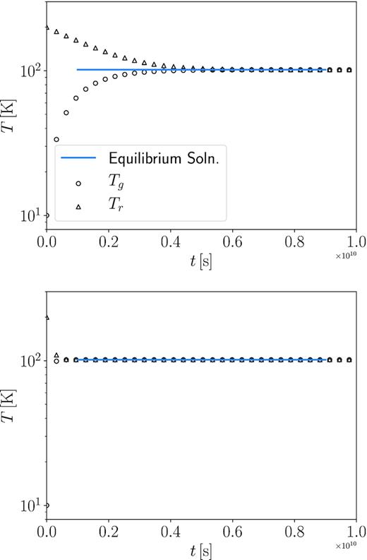
Gas (circles) and radiation (triangles) temperatures as a function of t for |$\kappa =1$| (top panel) and |$100\, {\rm cm^2\, g}^{-1}$| (bottom panel). The initial Tr = 200 K, while the initial gas temperature is Tg = 10 K. The solid blue line is the equilibration temperature of 101.7 K.
3.2 Momentum conservation
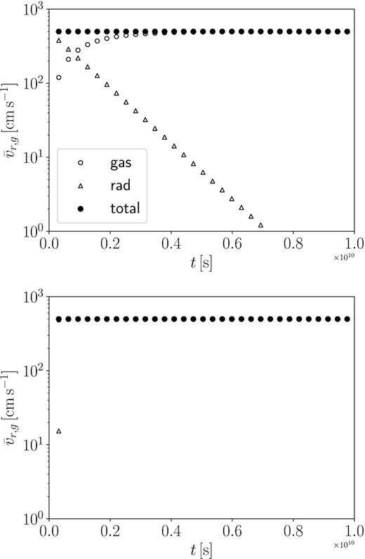
Gas (empty circles) and radiation (triangles) effective velocities as a function of t for |$\kappa =1$| (top panel) and |$100\, {\rm cm^2\, g}^{-1}$| (bottom panel). The effective velocity for the total momentum is shown by filled circles. The momentum is conserved to better than 4 × 10⁻⁴.
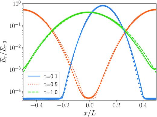
The radiation energy density, Er, as a function of position for three different times of t = 0.1, 0.5, and |$1\, L/v_{x,0}$|. The corresponding analytic solutions given by equation (50) are overplotted as solid, dotted, and dashed lines, respectively.
3.3 Dynamic diffusion
A dynamic diffusion test is useful for testing the diffusion of radiation in an optically thick moving medium where both the advection and diffusion of radiation occur simultaneously. Previously, JSD14 argued that the transport part of equation (10) should be split into a fluid advection term and a radiation transport term to reduce numerical diffusion for optically thick cells. Instead, we have adopted a van Leer second-order time integration, which allows us to pass this test without using the JSD14 split transport scheme.2
3.4 Crossing beams
The propagation of two beams of radiation in vacuum is a straightforward test, which can produce qualitatively wrong results depending on the RT method. For instance, M1 methods tend to merge two beams of radiation at a point where they intersect due to a single preferred direction in this moment method (JSD14). Short characteristics methods (Davis et al. 2012; Jiang et al. 2012) and time-dependent angular methods (JSD14), on the other hand, produce correct results.
In Fig. 4, we show the results of the crossing beam test in our MM implementation. Here, we set |$\bar{c}= 10\, {\rm km\ s^{-1}}$| in a box that is 16 pc on a side and fill it with 3 × 10⁵ particles by replicating a glass distribution of 4096 particles. We note that the actual values of the box and reduced speed of light is irrelevant here as the absorption and scattering opacities are minimal, e.g. τ < 1 across the box. We use 80 angles in the simulation to cover the unit sphere. In this simulation, we do not perform an implicit solve for the gas temperature as described in Section 2.3, but rather leave it fixed. This allows us to focus on the propagation of radiation. We place sources as cylindrical sources along z at |$(x,y) = (-10^{19},-10^{19})$| and |$(10^{19},-10^{19})\, {\rm cm}$| with directions of θ = π/4 and 3π/4 on the left and right cylinder, respectively. We use a radiation temperature of Teff = 200 K. Here θ is defined along the x–y plane. The opening angle is set such that cos δθ < 0.95, which picks out just two angles per cylindrical source. Finally, we place an absorbing boundary condition at y = 2 × 1019 cm and periodic boundary conditions in the x–z boundaries.
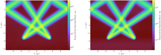
Projected Er for a stationary fluid and mesh (left-hand panel) and the moving fluid and mesh (right-hand panel). In the right-hand panel, the fluid moves in the +x-direction at a velocity of |$v=3\, {\rm km\ s^{-1}}$|, which is 30 per cent of the reduced speed of light |$\bar{c}$|.
In the left-hand panel, the fluid has zero velocity and we see that the results are qualitatively correct after several radiation crossing times. In the right-hand panel, the fluid moves in the + x-direction at a velocity of |$v=3\, {\rm km\ s^{-1}}$|, which is 30 per cent of the reduced speed of light |$\bar{c}$|. This motion of the fluid moves the cells in a MM code, and some effect in light propagation is expected when the velocity of the fluid approaches the reduced speed of light. Here we find that after beams have propagated, there is little difference between the case where mesh-generating points are static (left-hand panel) and where they are moving (right-hand panel) at 30 per cent of the reduced speed of light. Though we do not show it, we did find that the radiation front is distorted in the direction of the mesh-generating points’ motion. Finally, distortions on the propagation of the beams show up when the mesh generating points approach 50 per cent of the reduced speed of light or higher, which we also do not show. However, given the effect of slow MMs (relative to |$\bar{c}$|) on equilibrium radiation fields is small, the RSLA is excellent when |$\bar{c}$| is set to be few times faster than the fastest fluid velocity and/or mesh-generating points.
3.5 Shadow test
Like the crossing beam test, the shadow test has been used to demonstrate the ability of various methods (FLD, M1, RT, VET) to capture the qualitatively correct behaviour of photons propagating in multiple directions simultaneously. This test has been widely use to demonstrate the superiority of M1 methods to capture the shadow cast by one beam compared to FLD, which does not cast shadows (McKinney et al. 2014). However, M1 performs more poorly with more than one beam, e.g. multiple shadows. In particular, the closure used in M1 can only account for one direction of propagation. For more than one beam, the direction is then taken as the intensity-weighted direction, which is qualitatively incorrect. On the other hand, time-dependent methods (JSD14) or VET (Davis et al. 2012; Jiang et al. 2012) methods capture the correct qualitative dynamics.
We set up a multiple shadow simulation with a 16-pc side box and populate it with 3.1 M mesh-generating points. This simulation is larger than the others above because we want to capture the sharp transition between fluids of different densities. We set an ambient density of |$\rho =3\times 10^{-22}\, {\rm g\, cm}^{-3}$| with a mean opacity of |$\kappa _{\rm J}=100\, {\rm cm^2\, g}^{-1}$|, making it marginally optically thick, τ ≈ 1. The Planck opacity (corresponding to emission) is set much smaller |$\kappa _{\rm P}=10^{-2}\, {\rm cm\, g^{-1}}$|, so that there is negligible re-emission. As in the crossing beam test, we adopt periodic boundary conditions along the x- and z-axes. We use absorbing boundary conditions for the radiation and periodic boundary conditions for the gas. The exception is the lower y-boundary where we set the boundary to be a fixed radiation input field. The radiation is set at directions of θ = 0.98 (56°) and −0.98, measured from the y-axis, and the radiation temperature is Teff = 200 K. At (x, y) = (0, −3) pc, we place a dense elliptical tube that extends in the z-direction. We set the density of the tube to be 1000 times larger than the ambient density so that it is optically thick. The elliptical tube has a major axis of 4.8 pc and a minor axis of 3 pc, with the major axis oriented along the x-axis. We adopt the same opening angle of cos δθ < 0.98, which picks out just one angle. Finally, we place the absorbing boundary condition at the top and bottom (in y), but periodic elsewhere. We ignore the radiation coupling to the hydrodynamics, though the hydrodynamics are evolved.
In Fig. 5, we project Er for the multiple shadow test. The mulitple shadows cast by the tube are qualitative, which is expected. The umbra and penumbra are visible and follow our qualitative expectations. As argued in JSD14, these results are qualitatively superior to the M1 method, which casts only one shadow.
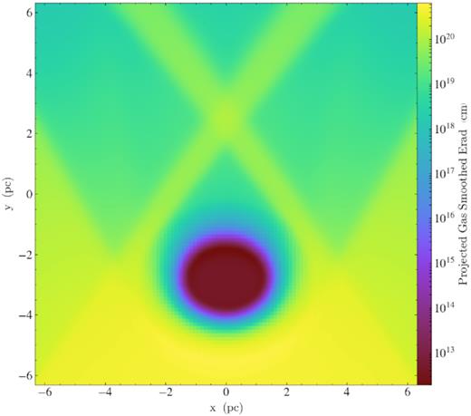
Projected Er for a multiple shadow test. Radiation is emitted with a radiation temperature of |$T_{\rm eff} = 200\, {\rm K}$| from the bottom boundary with angles θ = 0.98 (56°) and −0.98 from the y-axis. Two shadows will be produced and the shaded beams are also visible.
3.6 Linear wave
The radiative linear wave is a full end-to-end test of the full radiation hydrodynamics algorithm and, thus, we carry out the linear wave test in a three-dimensional domain based on the dispersion relation by Jiang et al. (2012) (see also Jiang et al. 2014; Zhang et al. 2018). As discussed in Jiang et al. (2014), the relevant parameters for this test are |$\mathcal {C} = c/c_{\rm s}$|, the ratio between the speed of light and isothermal sound speed, |$r = \bar{c}/c$|, the ratio between the reduced speed of light and speed of light, |$\mathcal {P} = P_{\rm rad}/P_{\rm g}$|, the ratio between the radiation and gas pressures, τλ = κρλ, the optical depth over one wavelength, and γ = 5/3, the adiabatic gas index.
The setup in manga assumes physical units, so we set up a uniform medium with background density |$\rho = 10^{-2}\, {\rm g\, cm}^{-3}$| and box size in the x-direction Lx = 3 × 1010 cm. The box size in the y- and z-directions are equal, Ly = L|${\rm z}$|, and set based on the resolution in the x-direction and scaled such that the total number of three-dimensional mesh-generating points remains approximately constant. These physical units are irrelevant to the problem once everything is scaled to the four parameters described above. We set up the mesh-generating points with a regular lattice structure, but perturbed randomly by 10 per cent of the grid spacing to ensure that there are no degeneracies in the Voronoi planes. We also fix the mesh-generating points in this test as the motion of the mesh-generating points (in the regularization step, see, e.g. Chang et al. 2017) produced a noise that can exceed the perturbation of the linear wave.
Setting the wavelength of the linear wave to be the size of the box in the x-direction, we adopt |$\mathcal {C} = 1.45\times 10^3$|, r = 10−2, and |$\mathcal {P} = 1$|. In other words, we use a reduced speed of light, which is 1 per cent of the speed of light, and a sound speed, which is ≈0.1 of the reduced speed of light. We also set the radiation pressure equal to the gas pressure. We have run tests with different r and |$\mathcal {P}$| and the results are consistent with the analytic results (using those parameters) that we describe below. We use the analytical solutions of Davis et al. (2012) for τλ = 10−2–102 to initialize a linear wave with a dimensionless amplitude of 10−3.
In Fig. 6, we compare the measured phase velocity, vph, in units of the isothermal sound speed, cs, and the measured damping rate, γ, from our manga simulation with an effective grid resolution of 160 in the x-direction with the analytic curves from Zhang et al. (2018). We measure the phase velocity and damping rate by evolving our linear wave for one isothermal sound speed crossing time and fitting the linear wave solution for the phase and amplitude. It is clear from this figure that the analytic results are captured with a high fidelity.
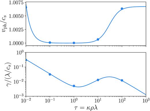
Phase velocity, vph = ωr/k, in units of the isothermal sound speed, cs (top panel), and damping coefficient, γ (bottom panel), in units of λ/cs for Prad = Pg, c/cs = 1.45 × 10³, and cr/c = 10−2 as a function of optical depth across a wavelength, τw. Solid dots are fits from the simulations.
In Fig. 7, we plot the error, ϵ (with arbitrary normalization), as a function of the number of grid points in the x-direction, e.g. the effective resolution. Here we define the error, ϵ, as the L1 norm between the analytic and numerical solutions after one isothermal crossing time. A fit to the error shows that the convergence of the radiative linear wave (in all optical thickness regimes) is approximately a power law with an index of −1. We confirm the second-order nature of the hydrodynamics solver by showing that the L1 norm of a pure acoustic wave has a power-law index of −1.74 with respect to linear resolution. This is nearly the same index found by Yalinewich et al. (2015), whose methods of gradient estimation we adopt in manga (Chang et al. 2017).
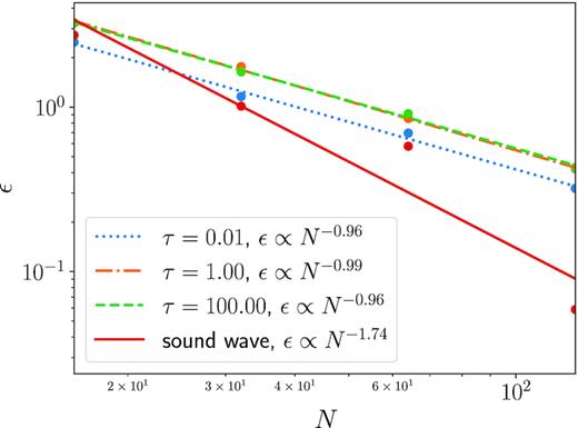
Error (as L1 norm) as a function of x-resolution, N, for τ = 0.01, 1, 100, spanning the range from optically thin to thick. We also plot the error for a pure acoustic wave that has an index of −1.74, which is close to the expected second-order convergence index of −2. The convergence of the radiation cases is consistent with first-order convergence.
Although the integration and reconstruction scheme might be expected to yield second-order convergence, the method is only formally first order since the implicit update of the radiation transfer source term is only first order in time. Hence, our first-order convergence is consistent with this expectation. Nevertheless, we note that JSD14 showed second-order convergence for the case of τ = 0.01 and |$\tilde{c} = c$|, which can be attributed to the limited impact of the radiation source term on the sound wave in this regime. Our convergence remains only first order for τ = 0.01 with either |$\tilde{c}=10^{-2} c$| or c, motivating a further study to see if we can improve convergence in this weakly coupled regime.
Finally, we explore the effect of mesh regularity on the convergence of our result as previously discussed by Pakmor et al. (2016a). In Fig. 8, we plot the L1 norm for the radiative linear wave with τ = 1 and the pure acoustic wave for a nearly Cartesian mesh (deviations in the mesh-generating points of 10−6 of the separation, dx) and two Cartesian meshes with deviation of 1 and 10 per cent of the separation. For the acoustic wave, we can see that increasing non-regularity of the mesh degrades the second-order convergence of the hydrodynamics solver, but the linear wave suffers no such degradation. Instead, its first-order convergence appears to be dominated by the radiation solver.
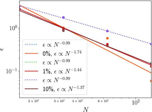
Error (as L1 norm) as a function of x-resolution for τ = 1 and the pure acoustic wave for a nearly Cartesian grid |$0{{\ \rm per\ cent}}$| deviation and two Cartesian grids with a Poisson deviation in the mesh-generating points of 1 and |$10{{\ \rm per\ cent}}$| of the separation, dx. The radiative linear wave is dominated by the first-order convergence of the radiation solver, while the second-order convergence of the sound wave is degraded by an increasingly non-regular mesh.
4 DISCUSSION AND CONCLUSIONS
We have adapted JSD14’s algorithm for radiation hydrodynamics based on solving the time-dependent RT equation to an unstructured MM and implemented it in the MM code, manga. We solve the specific intensities along different angles and integrate these intensities over angles to find the radiation energy and momentum source terms coupled to the hydrodynamic equations. We have tested our implementation on a set of simple problems. These test problems show that energy and momentum between radiation and matter is conserved by the implicit solver even when the coupling time between radiation and matter is much shorter than the characteristic time-step. Additionally, the crossing beam and multiple shadow tests demonstrate that the method produces qualitatively correct results in the optically thin limit when multiple sources and obstructions give rise to a complex radiation field. In particular, these latter two tests demonstrate the importance of the angular distribution of radiation in producing the qualitatively correct dynamics. As stated in JSD14, the principle advantage of this method is that the angular distribution of photons is calculated self-consistently. Because we do not use an ad hoc closure relation, as required in FLD and M1 methods, this method is generally superior in the optically thin case with complex radiation fields. Finally, we demonstrate the fidelity of our radiation hydrodynamics solver in reproducing an analytic results in the linear wave test and converging appropriately with a higher resolution.
As mentioned by JSD14, the method of solving the time-dependent RT equations is more straightforward to implement than the method of short characteristics as it does not require a global solver. In addition, JSD14 mentions that this method treats radiation and hydrodynamic variables on a similar footing. Thus, it is straightforward to extend it to curvilinear coordinate systems with non-uniform grids. Here, we recognized their insight by extending it to moving unstructured grids.
Our primary planned applications for this radiation module are dynamical stellar problems such as stellar mergers (Prust & Chang 2019) and tidal disruption events. Cases where radiation pressure blows the material away may require the development of a grid regularization scheme. Radiation momentum driving tends to push the material away from sources, which typically are a small fraction of the volume of a simulation box. As a result, MMs can quickly get distorted without some sort of mesh regularization that either keeps the volume or mass of each cell fairly regular or an algorithm to generate more mesh points to maintain mesh regularity (S10). In contrast, gravity tends to pull material from the entire simulation volume into small regions, so the need for such algorithms, while desirable, is not required. For this reason, we have refrained from simulating radiation feedback problems (Krumholz & Thompson 2012; Davis et al. 2014; Rosdahl & Teyssier 2015), which Kannan et al. (2019) have recently demonstrated using arepo-rt. We plan to implement a mesh regularization scheme for manga to address this need.
There are a number of improvements that would greatly improve the utility of the radiation solver. These include the inclusion of magnetic fields, alternative RT schemes, additional mesh generation/regularization improvements, and performance improvements. Here we note that the recent implementation of RT in arepo-rt (Kannan et al. 2019) contains an ionization solver. We have no plans to implement ionization in our current scheme as the relevant science questions that we are interested in do not require it.
Implementation of alternative RT schemes would permit comparison between these full angular schemes and moment schemes such as FLD or M1. Here we have mentioned the limitation of M1 in producing the qualitatively correct solutions to various test problems such as the crossing beam test and double shadow test. At the same time, the full angular implementation we use here suffers from angular discretization, which, for single sources, may be at a disadvantage compared to M1. A detailed comparison between different RT schemes for specific problems is a problem worthy of a further study.
Performance improvements for these various schemes are planned for the near future. Even in the RSLA, the reduced speed of light is usually at least a factor of a few faster than the fastest velocity, which limits the time-step. However, the RT solution can be greatly simplified compared to the hydrodynamic step in that the same Voronoi structure can be assumed to be constant across the step. As a result, sub-cycling the RT step may result in substantial computational savings, as Kannan et al. (2019) have recently implemented in arepo-rt.
The source code, test problems, and documentation for manga will be available with all the physics (MHD, radiation) in an anticipated future public release of changa. We hope that this code will find wide application in astrophysical problems. We encourage interested parties to contact us if they are interested in using manga before the public release.
ACKNOWLEDGEMENTS
We thank Norman Murray and Paul Duffell for useful discussions. We thank Jim Stone for useful discussions and for permission to use various code segments of athena and athena+ + in manga. We thank the anonymous reviewer for a constructive report. PC is supported by the NASA ATP program through NASA grant NNH17ZDA001N-ATP, NSF CAREER grant AST-1255469, and the Simons Foundation. SWD acknowledge support from NSF grant AST-1616171 and an Alfred P. Sloan Research Fellowship. YFJ was supported in part by the National Science Foundation under Grant No. NSF PHY-1748958. We also used the Extreme Science and Engineering Discovery Environment (XSEDE), which is supported by National Science Foundation (NSF) grant No. ACI-1053575. We also acknowledge the Texas Advanced Computing Center (TACC) at The University of Texas at Austin for providing HPC resources. which have contributed to the research results reported within this paper (http://www.tacc.utexas.edu). We also use the yt software platform for the analysis of the data and generation of plots in this work (Turk et al. 2011). The Flatiron Institute is supported by the Simons Foundation.
Footnotes
Following S10, we also include an evolution equation for entropy and switch between the two solutions based on either detections of shocks or explicit user input. In this work, we exclusively use energy evolution.
We note that athena+ + also implements a van Leer scheme (White et al. 2016) and its utility in reducing numerical diffusion in optically thick media has already been demonstrated in this code.
We set up a uniform medium with background density |$\rho = 10^{-2}\, {\rm g\, cm}^{-3}$|, box size in the x-direction LX = 3 × 1010 cm, and resolve it with 128 cells. We set x = 0 to be the centre of this domain. The box size in the y- and z-directions are equal, Ly = L|${\rm z}$|, and set to be boxes that are 3dx across, where dx is the separation of grid points in the x-direction. These physical units are irrelevant to the problem once everything is scaled to the four parameters described below in Section 3.6, e.g. |$\mathcal {C} = c/c_{\rm s}$|, the ratio between the speed of light and isothermal sound speed, |$\mathcal {P} = P_{\rm rad}/P_{\rm g}$|, the ratio between the radiation and gas pressures, and τ = κρL, the optical depth in the x-direction. We set up the mesh-generating points with a regular lattice structure, but perturbed randomly by 10−6 of the grid spacing to ensure that there are no degeneracies in the Voronoi planes. The optical depth of the entire box is set to be τ = 400. We set |$\bar{c}= c$|, cs = 0.1c, and the initial velocity of the flow to be vx, 0 = 0.1c. We do not evolve the hydrodynamic quantities and allow the mesh to follow the flow.
The initial profile of the radiation energy density and flux is set to be 48 and 49, respectively.As in JSD14, we limit the lower value of Er to be fixed by Er, 0exp (− 10) and, like the linear wave test discussed below, limit the number of angles to one per octant. We also ignore the diffusive flux term as in JSD14; we find it makes little difference. In the diffusion limit, the analytic solution is given by equation (50) in JSD14. In Fig. 3, we plot Er for the case of t = 0.1, 0.5, and |$1\, L/v_{x,0}$|. We overplot the analytic solution given by equation (50). This figure shows that our algorithm can calculate the diffusion and advection processes accurately without the splitting of the transport step as done in JSD14.


