


Abstract
Feedback from supernovae is often invoked as an important process in limiting star formation, removing gas from galaxies and, hence, as a determining process in galaxy formation. Here, we report on numerical simulations, investigating the interaction between supernova explosions and the natal molecular cloud. We also consider the cases with and without previous feedback from the high-mass star in the form of ionizing radiation and stellar winds. The supernova is able to find weak points in the cloud and creates channels through which it can escape, leaving much of the well-shielded cloud largely unaffected. This effect is increased when the channels are preexisting due to the effects of previous stellar feedback. The expanding supernova deposits its energy in the gas that is in these exposed channels, and, hence, sweeps up less mass when feedback has already occurred, resulting in faster outflows with less radiative losses. The full impact of the supernova explosion is then able to impact the larger scale of the galaxy in which it abides. We conclude that supernova explosions have only moderate effects on their dense natal environments but that with preexisting feedback, the energetic effects of the supernova are able to escape and affect the wider scale medium of the galaxy.
1 INTRODUCTION
Star formation and the feedback from young stars are the primary internal processes that can drive galaxy evolution (Schaye et al. 2015). These processes are interconnected as feedback can affect the local star-forming environment, as well as the large-scale interstellar medium (ISM) from which the next generation of stars form (Dobbs et al. 2014). The morphology and rate of star formation (and therefore stellar feedback) also depend on the large-scale structure and dynamics of the host galaxies.
Numerical simulations have been instrumental in helping us understand how star formation proceeds and the dynamical processes that contribute to the observed stellar properties from the origin of stellar clusters (Bonnell, Bate & Vine 2003; Smilgys & Bonnell 2017), the initial-mass function (Bonnell et al. 2001; Bonnell, Larson & Zinnecker 2007), the formation of high-mass stars (Bonnell, Vine & Bate 2004; Zinnecker & Yorke 2007; Krumholz et al. 2009; Smith, Longmore & Bonnell 2009; Kuiper et al. 2010), and the origin of binary and multiple systems (Bate, Bonnell & Bromm 2003; Bate 2012; Reipurth et al. 2014). At the same time, numerical simulations have been used to explore how the initial conditions for star formation arise due to large-scale flows, spiral shocks or other dynamical events in the galaxy (Dobbs, Burkert & Pringle 2011; Bonnell, Dobbs & Smith 2013; Dobbs et al. 2014; Smilgys & Bonnell 2016; Vázquez-Semadeni, González-Samaniego & Colín 2017).
Feedback from young stars, in the form of ionizing radiation, stellar winds, and ultimately supernova (SN) explosions, is often invoked as processes to limit the rate at which stars form, recycle molecular gas back into the ISM, as well as a significant source of kinetic energy into molecular clouds and the ISM (Krumholz et al. 2014). On larger scales, SN explosions are considered essential in regulating star formation and gas expulsion in galaxies, helping to explain the stellar mass function of galaxies (Schaye et al. 2015).
Including ionization and stellar wind feedback on smaller scales has shown that the local gas environment plays a crucial role in channelling the outflows through weak points in the surrounding clouds (Dale et al. 2005; Dale, Ercolano & Bonnell 2012), allowing the feedback energy to largely escape and leaving more massive clouds less affected than would be estimated (Dale et al. 2014; Dale 2017; Ali, Harries & Douglas 2018). Similar conclusions arise when SN feedback is invoked in dense, structured environments (Rogers & Pittard 2013; Körtgen et al. 2016) although in many studies resolution issues necessitate lower density, near-uniform environments and/or subgrid treatments (Agertz et al. 2013; Geen et al. 2015; Walch & Naab 2015; Rey-Raposo et al. 2017; Keller et al. 2014).
Including SN feedback on galactic scales (Yepes et al. 1997; Marri & White 2003; Scannapieco et al. 2006; Simpson et al. 2015; Smith, Sijacki & Shen 2018) has generally necessitated relying on subgrid physics or on underresolved simulations. Issues that arise include uncertainty over tuning the subgrid physics (Rosdahl et al. 2017), and initial losses (e.g. overcooling) due to the lack of resolution that artificially reduce the uptake of SN energy by the ISM (Katz, Weinberg & Hernquist 1996; Dalla Vecchia & Schaye 2012).
In this paper, we investigate the effects of SN explosions in a realistic star-forming molecular cloud, and how the SN’s evolution is affected by previous stellar feedback in the form of ionizing radiation and stellar winds.
2 NUMERICAL METHODS
2.1 Smoothed particle hydrodynamics simulations
To perform our simulations, we used the smoothed particle hydrodynamics (SPH) code sphNG (Benz 1990; Bate, Bonnell & Price 1995). SPH is a Lagrangian method for computational fluid dynamics. The fluid is represented as a set of particles whose properties (positions, velocities, internal energies, densities, etc) evolve according to fluid equations calculated over neighbouring particles using a smoothing kernel. Each particle is itself smoothed through the surrounding volume defined by its kernel, allowing interpolated fluid quantities to be determined at any point in space. Benz (1990) and Monaghan (1992) provide useful introductory overviews of SPH.
Particles in the simulation were evolved on individual time-steps (Hernquist & Katz 1989), but this is known to be a source of error in energy and momentum conservation (Saitoh & Makino 2009). The problem is most pronounced when particles on very different time-steps interact with one another: the time-stepping scheme may not allow particles with long time-steps, such as those representing slowly evolving ambient gas, to ever ‘feel’ the effects of passing short time-step particles, such as those in SN ejecta, which are themselves receiving energy and momentum contributions. To circumvent this problem, a development of the time-step limiter scheme similar to that described by Saitoh & Makino (2009) and Durier & Dalla Vecchia (2012) was employed. When deployed within the simulation code’s Runge–Kutta–Fehlberg integrator, this maintained a factor of at most 4 between neighbour particles’ time-steps to ensure momentum and energy conservation. The time-step limiter also includes an immediate reduction of time-steps when neighbouring particles violate the above condition, as can occur in strong shocks.
We used the Run I simulations of Dale et al. (2014) as the basis for our SN simulations. To briefly describe Run I, it used 106 particles to simulate a spherical centrally concentrated cloud of |$10^4 \, \mathrm{M}_\odot$|. The SPH gas particle mass was, thus, |$0.01 \, \mathrm{M}_\odot$|. The cloud was |$10\, \mathrm{pc}$| in radius and turbulently supported with an initial ratio of energies Ekin/|Egrav| = 0.7. The cloud was then allowed to evolve using the ionization scheme of Dale, Ercolano & Clarke (2007) and the winds of Dale & Bonnell (2008). Dynamically created sink particles (Bate, Bonnell & Price 1995) were used to represent forming stars.
Three variations on Run I were used as the initial points for our SN simulations. One, referred to henceforth as ‘DFB’ for dual feedback, had been run to the insertion point using the full feedback model, including both ionization and winds from the massive stars that formed. Another, ‘ION’, used only ionizing feedback. 'NFB' was a control run, which had included neither form of feedback and, thus, was evolved with hydrodynamics under gravity alone. For each of these initial conditions, two versions were run, one including the SN (with run names postfixed ‘-S’) and another control run without (postfixed ‘-N’). This allowed us to isolate the effects of the SN in each run by also following the events that would take place in its absence.
2.2 SN method
In each simulation, we inserted the SN at the position of the most massive sink particle. The ejecta mass was set to |$\approx 23.9 \, \mathrm{M}_\odot$|, |$25 {{\ \rm per\ cent}}$| that of the most massive sink in the original control run. While the most massive sinks in the two runs with feedback were at lower values (almost equal to two-third that in the no-feedback run), we opted to use this mass in all three set-ups in order for the SNe in each to more closely resemble one another. Using the higher mass progenitor also ensured the highest number of particles in the SN.
The SNe ejecta were directly inserted by creating new gas particles around the most massive sink in each simulation. The mass of that sink was decreased by the same amount. The particles were randomly positioned within a sphere of radius |$r_\mathrm{SN} = 0.1 \, \mathrm{pc}$|, and with a central hole of equal radius to the sink particle accretion radius (|$10^{-3}\, \mathrm{pc}$|). Any gas particles already inside the SN insertion region were removed and then reinserted alongside the SN particles to conserve mass. A total SN energy of |$10^{51}\, \mathrm{erg}$| was split between kinetic and thermal forms, with the velocities directed radially outwards from the SN centre.
We created SNe using several recipes for the distribution of energy in the ejecta. We found that using a 90 : 10 ratio of kinetic to thermal energy resulted in an exceptionally well formed shock forming from nearby swept-up material. However, the SN ejecta itself almost shattered on impact with this material, forming small cannonball-like clumps of approximately 50 particles, the same as sphNG’s target number of neighbour particles. In the end, we settled on a 50 : 50 split of kinetic and thermal energy, giving us a total of 5 × 1050 erg in each form.
To ensure a well formed shock, the kinetic energies assigned to the SN particles followed an r−1 radial profile with an inner core. This led the inner regions to catch up to the outer regions of the SN ejecta, creating a well-formed shell. The thermal energies were distributed uniformly.
In order to assign particles velocities according to the profile, we first had to choose the core radius rcore, and define the fractional core size fr = rcore/rSN. We also defined the ratio of specific kinetic energy at the SN edge to that in the core, fe = ek(rSN)/ek, core. For our simulations, we found fe = fr = 0.6 worked well in producing a dense expanding shell.
In its modern form, sphNG uses the grad-h formulation of SPH (see e.g. Price & Monaghan 2004), requiring that the gas-particle masses be constant. In order to assure that the simulations accurately captured the interaction between ejecta and environment, we increased the resolution of the full simulation. Thus, before the SN’s insertion, we split each original 0.01M⊙ gas particle into nine, giving a particle mass of |$0.00\bar{1}\, \mathrm{M}_\odot$|. This increased the number of particles inserted for the SNe from ≈2400 to ≈21 500 (neglecting any reinserted particles from the nearby medium).
2.3 Cooling
The internal energy of the gas in our simulations was allowed to evolve following the method presented in Vázquez-Semadeni et al. (2007). With this method, the time-scale required for each particle to reach its equilibrium internal energy was calculated, taking into account radiative and hydrodynamic heating and cooling, and an implicit integration towards equilibrium was then performed. The cooling curve of Koyama & Inutsuka (2002) was used for low temperature (T < 104 K) gas. The curve was extended to |$10^9\, \mathrm{K}$|, with a uniform cooling rate from |$10^4\, $| to |$2 \times 10^5\, \mathrm{K}$|. At higher temperatures, the cooling rate decreases as described by Dalgarno & McCray (1972) and Ferland (2003). The final cooling curve is, thus, similar in form to the solar abundance, |$z$| = 0, n = 1 or |$100\, \mathrm{cm}^{-3}$| curves of De Rijcke et al. (2013).
3 OVERVIEW OF EVOLUTION
The main goals of this study were to investigate how the feedback from the SN interacted with its natal cloud and how this interaction depended on any previous feedback in terms of ionizing radiation and stellar winds. The simulation without previous feedback, NFB-S, has the stars deeply embedded within the dense molecular gas. In contrast, both simulations with previous stellar feedback, ION-S where ionization is included and DFB-S, where both ionization and stellar winds are included, have the high-mass stars and the central regions of the cluster within an H ii region. The rarefied nature of the immediate environment is clearly significantly different from the highly structured nature of the dense gas in the no-feedback run and, thus, play important roles in shaping how the SN interacts with the environment and how the SN energy is able to escape from the cloud. As mentioned before, these initial conditions were derived from the Run I simulations of Dale et al. (2014). We will first discuss the two cases, with and without previous feedback, separately.
3.1 Evolution without previous feedback (Run NFB-S)
At the point of SN detonation in the no-previous-feedback simulation, NFB-S, the progenitor was a member of the star cluster embedded deep within the cloud’s dense core. This dense gas remained due to the lack of any kind of previous feedback. It confined the explosion and led to the formation and expansion of a blast wave. Densities of 10−21–|$10^{-19}\, \mathrm{g}\, \mathrm{cm}^{-1}$| in the vicinity of the explosion mean that the explosion converted from free expansion to the Sedov–Taylor phase within a distance of |$1\, \mathrm{pc}$|.
The environment was highly inhomogeneous leading to a blast wave that was far from spherically symmetric. In the xy-projection, shown in Fig. 1, we see two blasts expanding into lower density gas above and below the central dense region with the appearance of a large filament. This geometry of the feedback largely resembles the shape of the feedback bubble from ionization (and ionization plus winds) in the earlier Dale et al. (2014) study. The higher density filament seen in Fig. 1 was significantly more robust to the initial blast wave but affected over longer time-scales by the high pressure in the SN remnant. From other perspectives, however, the large filament is revealed to be the projection of a smaller more complex set of filaments within the cloud, and the SN did indeed expand in a single blast wave, albeit a highly asymmetric one. This SN then is not too dissimilar from those described by Haid et al. (2016), whose models show an SN expanding at different rates into cones of different densities.
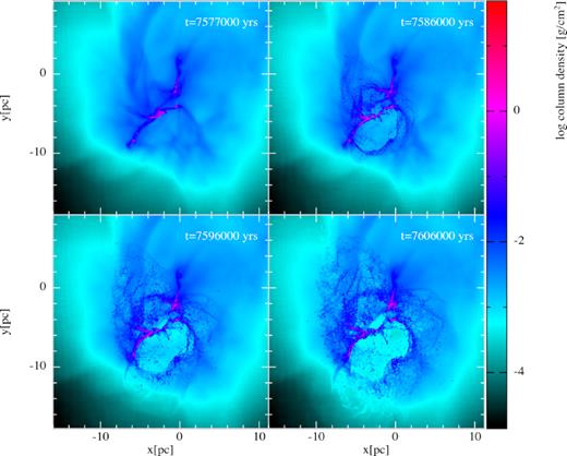
Evolution of run NFB-S, shown as column density in xy-projection. The SN progenitor was located in the densest regions at the centre of the cloud and is visible as the small high-density ball in the first panel. Due to its location, the explosion was confined and formed a large expanding bubble. The denser material constrained the explosion more effectively, giving it the appearance of a double-bubble in this projection in xz- and yz-projection, this is not the case as the progenitor was offset from the centre. While dense gas survived, its structure was markedly altered after the SN’s passage.
This behaviour can be seen more clearly in Fig. 4. The shock moved forwards slowly along the densest LOS such that it reached a distance of |$6\, \mathrm{pc}$| from the progenitor star’s position by the end of the simulation. The least dense LOS can be seen in the figure’s second panel to have not been substantially less crowded, reaching final column densities only an order of magnitude below those in the densest LOS. Nevertheless the difference was enough that the shock was driven forwards to nearly 50 pc. This preferential expansion into the paths of least resistance – lower density regions – will become even more prominent when ionization or stellar winds feedback is included in the pre-SN evolution.
3.2 Evolution with previous feedback (Runs ION-S and DFB-S)
Including earlier feedback in the pre-SN evolution had a significant effect on the overall evolution. This was due to the actions of the stellar feedback in creating escape routes in the cloud. Stellar feedback before the SN was implemented as either ionization alone or ionization alongside stellar winds. The cluster of massive stars in the deepest regions of the cloud acted as the source for this feedback, and as such was also the location of the SN. This meant that in both cases the SN exploded into a cavity partially surrounded by high-density molecular gas, the eroded remnants of the original cloud. In some cases, the boundary from ionized gas to molecular cloud was nearly flat, giving the dense cloud a wall-like geometry. Other geometries are pillar-like structures (one prominent example can be seen in run ION in Fig. 2 pointing from the lower left towards the central cluster) and small droplet-like clouds completely surrounded by ionized gas (easily seen at |$y \approx -20 \, \mathrm{pc}$| in DFB in Fig. 3). The state of the two simulations at the point of SN detonation can be seen in the first panels of Figs 2 and 3.
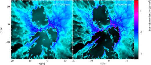
Evolution of run ION-S, showing column density in xy-projection at the point of SN detonation and 2.87 × 10⁴ yr later. The SN is seen as the small high-density sphere in the lower cavity (note that this structure is a projection effect only). The changes are not nearly as drastic as those seen in Fig. 1. The SN removed some ionized gas from the cavity, leading to a drop in density, and further sculpted and slightly increased the density in the walls. The cavity itself was slightly larger, most visible in the shape of the topmost cavity walls. The overall effect seems to simply be a continuation of the earlier ION’s action. Beyond the lower left limits of the plot is an expanding low density shell expelled by the SN which left the cloud while sweeping up only low-density ionized gas.
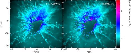
Evolution of run DFB-S, showing column density in xy-projection at the point of SN detonation and 2.87 × 10⁴ yr later. The SN is just visible as the small high-density sphere in the central cavity. This view is more zoomed out than that shown in Fig. 2, allowing the density peak in the blast wave to be visible at negative y, where it has essentially left the cloud unimpeded. Overall, the impact of the SN was very similar to that in run ION-S in the slight increase in density in the cavity walls. Very slightly different was that the low density gas left in the cavity by the SN’s wake was actually an increase in density, as it had actually been vacuum at the time of insertion.
Although the central cavities appear closed, particularly in the ION simulations, which appear to show two bubble-like structures, this is only a projection effect in the column density. In order to quantify the differences in the non-feedback and feedback initial conditions, we investigated what fraction of the sightlines as seen from the SN were open, which we defined as having column densities ≤10−4 g cm−2. This corresponds to the minimum column density in the no-feedback (NFB-S) initial conditions as well as a critical column density allowing high-velocity outflows (see Fig. 6).
In each of the three SN simulations, the sky from the position of the progenitor sink particle was split into 768 HEALPix pixels (Górski et al. 2005), the centre of each pixel defining an LOS. While none of the 768 HEALPix sightlines were open in the no-feedback run (NFB-S), the previous feedback runs had 67 and 75 per cent of the sky open in the ION-S and DFB-S, initial conditions, respectively, as seen from the SN’s position. These large portions of open sky in the feedback runs formed the preferred pathways for the SN’s expansion. In ION-S, it was only low-density ionized gas that was initially swept up by the ejecta. In DFB-S, the situation was even more extreme, the higher level of feedback in the original simulation led to the region around the cluster being completely vacated of gas, i.e. it fell within no gas particle’s smoothing kernel.
In general, the two feedback runs, ION-S and DFB-S, experienced very similar effects from the SN. The edges of the dense molecular clouds facing the SN were compressed by the shock at the point that it met them, but the large-scale and rapid destruction seen in Run NFB-S was entirely absent. Small clouds entirely or nearly entirely overrun by the explosion were compressed inwards towards their centres. Some ablation takes place along cloud edges. The latter two effects can be seen in the long pillar reaching into the centre of the two plots in Fig. 2 from the bottom left-hand panel. Finally, the central low-density region in both runs expanded slightly.
3.3 Shock expansion rate
Examining Fig. 4 shows how different the rate of the shock’s expansion is, depending on whether early feedback was included in the simulations. The shocks are very asymmetrical so we calculated the shock expansion rates in two directions, defined as having the highest and lowest column densities according to the HEALPix method outlined above. The expansion rates were then calculated along the most and least dense LOSs in order to take account of the highly inhomogeneous surroundings. The shock positions were defined by finding the position with the steepest radial entropy gradient (excluding the noisy low-density cloud boundary). The bottom plot compares the column density found along each of these paths at the SN detonation time.
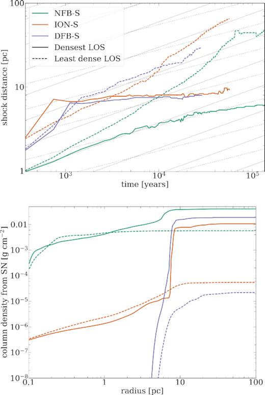
The upper plot shows the expansion of the shock driven by the SN. The position of the shock is shown along two line LOSs for each simulation – these were determined by taking the simulations at |$t_\mathrm{SN} = 0\, \mathrm{yr}$| and finding the most and the least dense LOS from all those given by the centres of 768 HEALPix pixels (Górski et al. 2005), using the SN as the origin. The solid and dashed grey lines respectively show the Sedov–Taylor and pressure-driven snowplough expansion rates. The lower plot shows the column density from the SN as a function of distance along each corresponding LOS. The expansion of the SN shock was slowest in NFB-S, and, in particular, along the densest LOS where it failed to move beyond |$6\, \mathrm{pc}$| in over 105 yr. At the same time, it moved to almost |$50\, \mathrm{pc}$| along the path of least resistance (though it should be noted that the method for determining the position of the shock began to break down at around this point). Both runs with previous feedback, ION-S and DFB-S, show that the expansion of the shock was halted along the densest LOS, where, as the second plot shows, the column density jumped at the point of entry to the walls around the central cavity. On the other hand, the SN freely expanded along the paths where the column density grew slowly and there were no sudden jumps in density.
The shock expanded continuously for both LOSs in the no previous feedback run, Run NFB-S. Expansion was slow along the densest LOS and it continued to decelerate until by the final time reached in this simulation, |$1.35\times 10^5\, \mathrm{yr}$|, it had only reached a distance of |$6.09\, \mathrm{pc}$| from the SN progenitor’s original position. Interestingly, the expansion rate along this LOS was originally close to the Sedov–Taylor rate |$r \propto t^{2/5}$| while, by |$10^4\, \mathrm{yr}$| it transitioned to a slope more similar to the pressure-driven snowplough rate of |$r \propto t^{2/7}$|; these two slopes are respectively shown in Fig. 4 as the solid and dashed grey lines. That any match is found at all is surprising as these rates would be expected to apply only to expansion into a uniform density medium. This transition may have been driven by an increase in radiative losses as the shock moved into denser gas as seen from around |$5\, \mathrm{pc}$| along this LOS in the lower plot of the figure.
The shock in Run NFB-S moved outwards much more quickly along the least dense LOS. By the same final, time it had reached a distance of |$47.6\, \mathrm{pc}$| from the initial position. Our method for finding the shock position began to break down, however, at later times when it began to move through the outer regions of the cloud, as can be seen by the strange behaviour of the data in Fig. 4, and as such we would not rely on it. The general behaviour of fast expansion can still be reliably taken. Along this LOS, there is no clear relation to the expansion rate of either the Sedov–Taylor or the pressure-driven snowplough phases.
It is immediately apparent that the shock expansion was initially much faster in Runs ION-S and DFB-S, where previous stellar feedback had at least partially cleared the vicinity of the SN progenitor. Notably in these two runs, the shock nearly stalled in the densest LOSs once a distance of around 6–7 pc was reached, while the expansion in the least dense directions continued allowing the SN energy (and pressure) to be released. Examining the lower plot of Fig. 4, one can see that there are very large jumps in column density at the corresponding distance, matching the point where the LOS entered one of the walls of molecular gas surrounding the central cavity. Expansion did continue beyond this time but very slowly. The least dense LOSs, which passed only through ionized gas (and, as previously noted, vacuum in the central regions of DFB-S), allowed the shock to continue advancing at a rapid pace.
4 EFFECT OF THE ENVIRONMENT ON SN OUTPUT
Our goal is to understand how the distribution of nearby molecular gas, in turn, affects the distribution of the initially isotropic output from the SN. It is clear from the previous section that the SN expansion rate is very different, depending on the direction. Here, we look to investigate how the environment affects the kinetic energy and momentum deposition in the cloud.
4.1 Large-scale distribution of output
To understand better how the SN propagates through the cloud, Fig. 5 shows the angular distribution of kinetic energy across the sky from the position of the SN progenitor. The radial kinetic energy, that is to say, the kinetic energy calculated using only the radial component of the velocity, was calculated for each SPH particle making up the ambient gas and then added to whichever of the 12 288 HEALPix pixels (Górski et al. 2005) in which it was located.
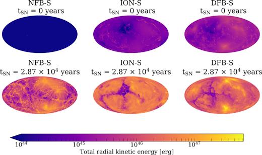
Distribution across the sky of radial kinetic energy in the ambient (non-SN ejecta) gas.
From Fig. 5 we can see that there was initially much more kinetic energy in the two runs, which had experienced earlier feedback, as would be expected. After the SN, a large amount of kinetic energy was distributed across the sky in the no-previous-feedback simulation NFB-S, in a complex filamentary structure with significant voids where little kinetic energy is deposited. Of greater importance are two large regions of high energy, and it is at these positions that the SN ejecta was able to break out of the cloud as was seen in the later times, shown in Fig. 1.
The kinetic energy was distributed much more smoothly across the sky in Run ION-S, where ionization had previously cleared the inner regions. There is also a very large area of low energy located close to the centre of the plot for |$t_\mathrm{SN} = 2.87\times 10^{4}\, \mathrm{yr}$|. Four ‘arms’ spread from it. Small regions of low kinetic energy are scattered elsewhere across the sky. These all correspond to dense clouds of varying size and shape, which have been able to shield themselves from the SN and so have not received much (or any) kinetic energy from the explosion.
Run DFB-S shows a cross-shaped structure of low-kinetic energy at the later post-SN time, roughly corresponding with the large low kinetic energy region seen in ION-S. The structure is, however, thinner and covers less of the sky, reflecting the reality that this simulation was previously bombarded with winds as well as ionizing radiation, leaving less material able to self-shield from the SN. Interestingly, there are two areas of higher kinetic energy closely corresponding those seen in NFB-S. Preferential channels for the escape of the SN ejecta and energy still exist, and since all simulations were evolved from the same initial seed, it should be expected that some similarities between them will remain.
4.2 Local energy deposition
We have seen how the energy deposited in the surrounding cloud is very asymmetrical and depends on the pre-SN structure extant in the environment. Globally, the three simulations’ initial conditions vary by the presence and volume of escape channels carved out by earlier feedback. In this subsection, we examine how individual mass elements were affected by the SN and how this depended on their local shielding from the SN. For each gas particle, we calculated the column density Σ between the location of the particle and the SN, with this value acting as a proxy for ‘exposure’ to the SN. Thus, a low-Σ particle could be described as being exposed to the SN, independent from its distance, while a high-Σ particle was shielded from the explosion.
Fig. 6 shows phase diagrams for gas particles in the three simulations, plotting the ‘kick’ ||$v$|r − |$v$|r, initial| received by each particle against the initial exposure Σinitial to the SN. The kick is simply the absolute change in the particle’s radial velocity with the SN at the origin. The initial time of the SN explosion was at tSN = 0 yr, while the kicks were found for tSN = 2.87 × 10⁴ yr (the end time of DFB-S). Histograms formed by compressing the phase plot in each direction are also shown. The initial SN particles are not shown in Fig. 6 as they have no values for Σinitial.
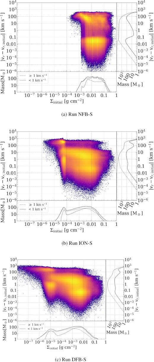
Phase diagrams at |$2.87 \times 10^4 \, \mathrm{yr}$| showing the LOS column density from the SN and the change in radial velocity for all gas particles in the cloud (i.e. the SN ejecta is excluded). The bottom and right-hand panels contain the same information compressed to one dimension. The bottom histogram of Σinitial shows the total and also two histograms for gas whose radial velocities changed by more or less than |$1\, \mathrm{km}\, \mathrm{s}^{-1}$|, itself marked on the main histogram. The right-hand histograms also show forward and reverse cumulative sums of the distribution.
The diagram for the no previous feedback simulation, NFB-S, is the simplest to understand. The phase diagram shows two populations of particles: the particles in one received changes in radial velocity barely exceeding |$0.1\, \mathrm{km}\, \mathrm{s}^{-1}$|, while in the other they reached several hundred |$\mathrm{km}\, \mathrm{s}^{-1}$|. The high-kick group was not present initially, but forms as the SN expands and interacts with the surrounding material. Particles across the whole range of Σinitial were able to reach the highest velocities as the explosion was confined within the molecular cloud; it was possible for anything nearby to become swept up in the shock irrespective of its initial environment. There is a significant increase in the particle density at lower Σinitial in this high-kick group, as can be seen in the corresponding histogram; the higher kick particles were more likely to be more exposed in the initial conditions. In other words, there is still a preference for the expansion of the shock to progress along lower density paths.
The plots for the previous stellar-feedback runs, ION-S and DFB-S, are more complex. The two simulations show similar distributions of particles across four groupings in the phase diagrams, although the groups spread to lower Σinitial in the dual stellar feedback run, DFB-S. A significant fraction of the gas in both simulations is found at high initial column densities, Σinitial, and the bulk of this gas receives only moderate kick velocities from the SN. The particles here made up the dense remnants of the cloud between the escape channels, carved out by ionization and winds. Maximum-velocity kicks of this dense gas were some 10’s of km s−1 with much of it getting kicks of less than ≈0.1 km s−1. The highest kicks extending up to nearly |$10^3\, \mathrm{km}\, \mathrm{s}^{-1}$| were experienced by particles in the low-Σinitial (exposed to the SN) group. Ionized gas still untouched by the shock at tSN = 2.87 × 10⁴ yr can be seen in the lower left group of particles, while those particles through which it has already passed can be seen directly above at the highest values for ||$v$|r − |$v$|r, initial| between 100 and |$10^3\, \mathrm{km}\, \mathrm{s}^{-1}$|.
The contrast between the simulation without previous feedback, NFB-S, and the two with previous feedback, ION-S and DFB-S, is in which material received large kicks to their radial velocities, and the magnitude of those kicks. With no previous feedback, in NFB-S, all the gas around the SN could receive increases to their radial velocities of up to several hundred |$\mathrm{km}\, \mathrm{s}^{-1}$|, though the majority of the fastest moving material was the most exposed to the SN. The reverse cumulative histogram on the right-hand panel of Fig. 6(a) shows that 103 M⊙ of the total 104 M⊙ in the cloud was accelerated by at least |$100\, \mathrm{km}\, \mathrm{s}^{-1}$|.
When ionization and winds were allowed to shape the ISM in ION-S and DFB-S, the least exposed (highest Σinitial) gas, within dense molecular clouds, received at most of the order of |$10\, \mathrm{km}\, \mathrm{s}^{-1}$|. Only the very low Σinitial ionized gas could be pushed to radial velocities similar to or higher than those seen in NFB-S. This can be seen clearly in Fig. 7 that shows the mass distribution as a function of the velocity kick received from the SN over the 2.87 × 10⁴ yr of the various simulations. The no-previous feedback run shows a double-peaked distribution with nearly equal parts receiving essentially no kick and kicks of some 10–100 km s−1 with the high-kick population coming entirely from the exposed gas with low-column densities to the SN. The previous stellar-feedback runs show a wider distribution of kick velocities, with a smaller total-gas mass at kick velocities above 1 km s−1, but significantly a small peak of the mass at very high velocities of >100 km s−1. This shows the effect of the channelling of the SN explosion by the previous feedback such that a smaller fraction of the mass then contains a much higher fraction of the SN’s kinetic energy. This will increase the amount of energy that can escape the natal cloud in these simulations.
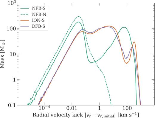
The distribution of mass is shown as a function of the radial velocity kick, defined as the absolute change in a given particle’s radial motion between the start of the simulation and the measurement time at |$2.87 \times 10^4 \, \mathrm{yr}$|. The plot shows the comparison of the three SN simulations and one control run without SN explosion. The SN generates significant kick velocities of up to several hundred km s−1. The high-kick velocities are almost entirely from gas particles that are exposed, i.e. low |$\Sigma \le 4 \times 10^{-3}\, \mathrm{g}\, \mathrm{cm}^{-2}$|. The no-previous-feedback simulation has a bimodal distribution as more mass is swept up by the SN but to lower velocities. The two cases, with previous feedback, have more mass given moderate (several km s−1) but also significant peaks of mass at the highest kick velocities.
4.3 Mass-loss
The SN’s ultimate impact on the larger scale environment depends on how much mass and energy escapes the natal molecular cloud. We measure the mass-loss as the time derivative of the mass contained within 10 pc of the SN, as seen in Fig. 8. All three simulations show initially low mass-loss rates with the non-previous stellar-feedback run (NFB-S) having effectively zero mass-loss rates, whereas the ION-S and DFB-S have initial mass-loss rates of |$(1\!-\!2) \times 10^{-3} \, \mathrm{M}_\odot \, \mathrm{yr}^{-1}$|.
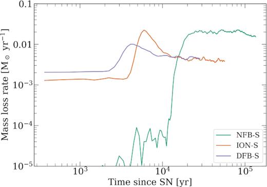
The mass-loss rate, through a sphere of 10 pc centred on the SN progenitor, is shown for the full simulation time in each of the three runs. The pre-SN feedback runs (ION-S and DFB-S) have initial mass-loss rates of |$\approx 10^{-3}\, \mathrm{M}_\odot \, \mathrm{yr}^{-1}$|. These temporarily (few × 103 yr) increases to values of |$(1\!-\!2) \times 10^{-2}\, \mathrm{M}_\odot \, \mathrm{yr}^{-1}$| as the SN shock passes 10 pc. In contrast, the no feedback run (NFB-S) has essentially zero mass-loss rate until the SN shock reaches 10 pc, but then sustains a high mass-loss rate of |$\approx 2 \times 10^{-2}\, \mathrm{M}_\odot \, \mathrm{yr}^{-1}$| over many times around 104 yr. This shows that the structures due to the previous feedback are able to channel the SN outwards, allowing it to escape without significantly affecting the remaining cloud.
The mass-loss rates increase significantly as the SN shock passes reaches 10 pc (see Fig. 4). This occurs after 2600 yr in the DFB-S simulation with a peak mass-loss rate of |$1.0 \times 10^{-2}\, \mathrm{M}_\odot \, \mathrm{yr}^{-1}$| at 4100 yr. In the ionization simulation (ION-S), the SN shock required longer (3700 yr) to reach 10 pc but then produced a higher peak mass-loss rate of |$2.2 \times 10^{-2}\, \mathrm{M}_\odot \, \mathrm{yr}^{-1}$| at 6000 yr. Finally, in the no previous feedback run (NFB-S), the SN shock does not reach 10 pc until 11 500 yr but then produces a high, and sustained mass-loss rate of |$2 \times 10^{-2}\, \mathrm{M}_\odot \, \mathrm{yr}^{-1}$| over 105 yr.
It is clear that the existence of significant holes in the cloud due to the previous feedback events are able to channel the SN shock more quickly out of the cloud, and, hence, less mass is lost from the inner 10 pc than in the case where the SN shock has to propagate through a pristine molecular cloud. Even though more mass is lost from the NFB-S case, it should be noted that this cloud has not already lost significant mass from any previous feedback event. The higher mass-loss from the NFB-S simulation (≈2 × 10³ M⊙) succeeds in reducing the cloud mass to be comparable with the initial mass in the ION-S cloud. Initial masses for the three clouds were NFB-S: 4604 M⊙; ION-S: 2620 M⊙; DFB-S: 1290 M⊙.
We can conclude that clouds with previous stellar feedback are more porous, with preexisting channels allowing the SN explosion to escape more quickly, and without sweeping up as much mass as than would be the case when no previous stellar feedback occurred. This is important in allowing the SN to escape the natal environment and this affects the larger scale in the galactic ISM.
4.4 Energy loss
As well as examining how mass was removed across the three simulations, it is also beneficial to look at how energy was lost. The sum of the kinetic and internal energies is plotted as a function of time for the three SN simulations (Fig. 9). The energy is calculated within radii of 10 and 50 pc, the latter intended to capture the SN even after it has escaped the cloud. The initial energy deposition in the SN was set at 1051 erg.
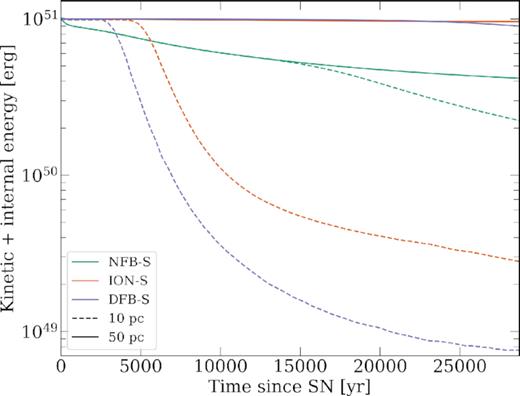
This figure plots against time the summed kinetic and internal energy contained within spheres centred on the SN of radius 10 and 50 pc. Energy on small scales (10 pc) is lost most quickly in the feedback runs, ION-S and DFB-S, as the ejecta and swept-up material carried energy outwards to larger distances. However, on larger scales (50 pc) more was lost in the feedback run in which the energy was thermalized in the shock’s interaction with dense cloud material and then lost radiatively.
The combined kinetic and internal energies within 10 pc are all seen to decrease once the SN shock passes this distance, as seen in Figs 4 and 8. This occurs first for the dual feedback run (DFB-S), then later for the ION-S and last for the no previous feedback run (NFB-S). Once the shock has passed through the inner regions of the cloud, the energy drops rapidly leaving the remnant, well-shielded portions of the cloud largely unaffected. This is aided by the existence of the channels eroded into the cloud due to the previous feedback.
In contrast, the SN shocks do not reach 50 pc over the time-scale of the simulations, so the combined kinetic and internal energy then measures the energy conservation of the SN as it expands in the cloud. What is most important is that the combined kinetic and internal energies are near constant for the two previous feedback simulations (DFB-S and ION-S), whereas there is a significant decrease for the no previous feedback simulation (NFB-S). This occurs from the initial stages of the simulation, well before the shock has reached 10 pc. Without any previous feedback, there are no well-formed channels in the cloud through which the SN can escape. Instead it needs to create these channels in the weakest regions of the cloud with low column densities. This creating of the outflow channels involves sweeping up more of the gas and distributing the SN energy into a larger mass distribution. When this occurs, more of the internal energy is able to escape through radiation from this larger, and, hence, cooler, mass distribution. Hence, in Fig. 9, the no previous feedback simulation has already lost over half its combined kinetic and internal energies in the first 25 000 yr from the explosion. The no previous feedback simulation was followed much further than the other simulations. Over the full 120 000 yr, we see that the internal energy decreases to ≈5 per cent of its peak value whereas the two feedback runs show negligible loss of internal energy over their full runs.
This issue is generally referred to as overcooling and is seen as a resolution limitation in cosmological simulations. Here we can see that even at high resolutions this can be an effect but that with realistic initial conditions where previous stellar feedback has created outflow channels in the cloud, the SN can readily escape the dense regions without sweeping up too much mass and, hence, suffering from overcooling and an excessive loss of energy.
It is worth noting that the SN remnant remains very hot even in the cases where significant energy is lost. Fig. 10 shows a cross-section of the density and temperature in the region for the no feedback (NFB-S) and the ionisation (ION-S) cases. Temperatures in excess of 106 to 107 K are present in the feedback bubbles. The remaining dense pre-SN gas is very cold and the contrast between the two highlights how this structure coexists in the region, while the SN eject escapes through the weak points in the cavity walls. The temperatures are slightly lower in the feedback bubble for the no previous feedback case as the SN had to sweep up more material in its path and, hence, increase the cooling. The ionization and dual feedback simulations have the highest temperatures in the feedback bubble due to the lower densities in the pre-SN cavity created by the earlier feedback mechanisms.
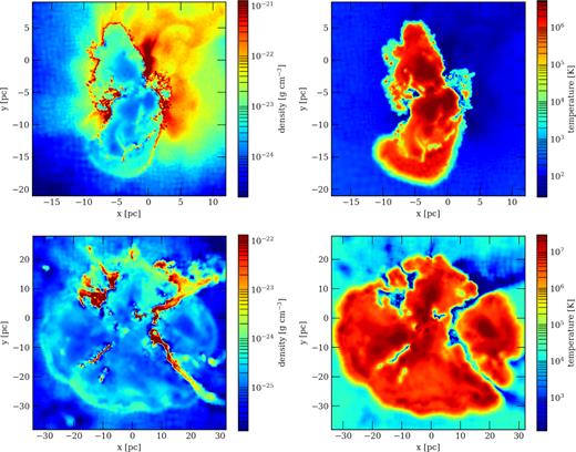
A cross-section of densities (left-hand panel) and temperatures (right-hand panel) of run NFB-S (top) and ION-S (bottom) are shown at 2.87 × 10⁴ yr after SN explosion. The high-density gas is from the pre-SN environment and remains cool, whereas the cavities are filled up of low-density gas at temperatures in excess of 107 K. Overcooling of the SN remnant is not occurring in this simulation. The slightly lower temperatures in the no feedback simulation (NFB) are due to the larger amount of mass that has been swept up in the explosion. The limit of the SN explosion is clear in both cases as is the effect of the ionising feedback in creating a large cavity for the SN to explode into.
5 DISCUSSION
One of the surprising results from these simulations is that the SN explosion, with many orders of magnitude more energy than the full gas cloud with its embedded stellar cluster, does not completely destroy the cloud. Instead, it creates channels, or employs already created channels due to previous stellar feedback, and largely escapes the dense cloud. The fact that the cloud can channel the SN outflow is due to the large gas pressure in the cloud such that the dense filaments are able to withstand the onslaught and shield much of the cloud. In the case where channels have already been formed by previous feedback, the SN can quickly escape the inner regions that reduces the thermal and kinetic pressures. It is clear from the kick velocities received from the SN that the dense shielded gas is largely unaffected by the SN. Feedback, hence, has little effect on nearby ongoing star formation.
In contrast, these simulations show that the exposed gas at low column densities is very much susceptible to the effects of the feedback. Exposed gas within the clouds at column densities Σ < 10−4 g cm−3 can be swept up and removed from the cloud. With preexisting channels created by stellar feedback, the mass swept up is reduced that allows more of the SN energy to escape unaltered by the dense cloud. The radiative losses from cooling by the denser gas is reduced and the full impact of the SN is permitted to leave the cloud and directly impact on the large-scale environment of the galaxy. It can, thus, have a significant effect on star formation on larger scales by energizing of the ISM of the galaxy.
It should be noted that the results presented here are for moderate mass clouds of only 104 M⊙ and that larger clouds with higher escape velocities are more robust against earlier forms of feedback (Dale et al. 2012). Such clouds may have more contained inner cavities from previous feedback events and, hence, act to better constrain the SN explosion to act within the cloud, and, hence, comparable to the no feedback run run presented here. The inner regions where ionization and winds will have created cavities, will most likely be comparable to the previous feedback runs in our 104 M⊙ cloud.
Of further note is the effect of resolution in simulating feedback from SN into larger scale simulations. Generally, such simulations will be resolution limited and unable to resolve the structure in the pre-SN cloud, be it generated by turbulence or earlier feedback events. The surroundings will then be typically more uniform and of lower median densities, allowing the SN to sweep up more of the material. This would then result in a stronger local effect of the SN feedback, destroying the local cloud, but higher cooling rates and energy losses and typically a lower effective feedback on larger scales. This was evident in our earlier simulations where we did not include particle splitting, and should remain a concern to all studies that include feedback into the ISM.
6 CONCLUSIONS
We have shown that resolving the natal environment, and including previous stellar feedback, is essential to accurately model the impact of SNe on their immediate and even larger scale environment. Realistic natal environments include significant dense gas structures and filaments that can act to channel the SN outflow through the weaker regions of the cloud with lower column densities. The SN’s energy is very preferentially deposited in these regions with lower column densities, i.e. less shielded from the SN. This asymmetrical ejecta leaves the dense, shielded, regions largely unaffected by the SN, as has been seen in the case where only stellar feedback is modelled (Dale et al. 2005; Dale 2017).
When previous stellar feedback events are included, the preexisting channels are well formed, allowing a more rapid and efficient escape of the SN energy and ejecta, with less gas mass being swept into the shock. The SN energy is then deposited in less mass, allowing the SN shock to leave the cloud faster, and to lose less energy due to cooling processes that would occur in a higher mass ejecta. We have considered only relatively moderate mass clouds (104 M⊙) that are most susceptible to pre-SN feedback (Dale et al. 2012). SN in larger mass clouds is likely to have central regions similar to our previous feedback runs, while the outer areas of the cloud would more closely resemble the no previous feedback case.
These results imply that modelling the natal environment of SNe is crucial in order to model their energetic coupling with the ISM at the correct scales. When stellar feedback is included, most of the energy of the SN can escape its natal molecular cloud and can, thus, impact lower density gas at larger distances in the ISM. This will have important consequences for galaxy formation and evolution.
ACKNOWLEDGEMENTS
WEL and IAB acknowledge funding from the European Research Council for the FP7 ERC advanced grant project ECOGAL. This work used the compute resources of the St Andrews hpcCluster Kennedy, and the DiRAC Complexity system, operated by the University of Leicester IT Services, which forms part of the STFC DiRAC HPC Facility (www.dirac.ac.uk). This DiRAC equipment is funded by BIS National E-Infrastructure capital grant ST/K000373/1 and STFC DiRAC Operations grant ST/K0003259/1. DiRAC is part of the National E-Infrastructure.
