


ABSTRACT
We use H i and H2 global gas measurements of galaxies from xGASS and xCOLD GASS to investigate quenching paths of galaxies below the Star forming main sequence (SFMS). We show that the population of galaxies below the SFMS is not a 1:1 match with the population of galaxies below the H i and H2 gas fraction scaling relations. Some galaxies in the transition zone (TZ) 1σ below the SFMS can be as H i-rich as those in the SFMS, and have on average longer gas depletion time-scales. We find evidence for environmental quenching of satellites, but central galaxies in the TZ defy simple quenching pathways. Some of these so-called ‘quenched’ galaxies may still have significant gas reservoirs and be unlikely to deplete them any time soon. As such, a correct model of galaxy quenching cannot be inferred with star formation rate (or other optical observables) alone, but must include observations of the cold gas. We also find that internal structure (particularly, the spatial distribution of old and young stellar populations) plays a significant role in regulating the star formation of gas-rich isolated TZ galaxies, suggesting the importance of bulges in their evolution.
1 INTRODUCTION
Observations have shown a strong correlation between global estimates of star formation rate (SFR) and stellar mass (M*) for populations of galaxies, commonly referred to as the ‘star-forming main sequence’ (SFMS, Brinchmann et al. 2004; Elbaz et al. 2007; Salim et al. 2007). The tightness of the SFMS suggests that star formation proceeds in a fairly universal and relatively calm mode, without significant deviations in SFR (Noeske et al. 2007). In an idealized completely isolated galaxy, secular evolution will produce this smooth and gradual evolution as stellar mass grows, gas is consumed, star formation diminishes, and optical colour becomes redder. Here, the SFR would depend largely on the available gas, and the two would decline hand-in-hand until the galaxy becomes red and fully dead.
In reality, galaxy evolution is more complex, as most galaxies do not spend their entire lives in isolation. They can merge or interact with other galaxies or dark matter haloes, which open up further evolutionary pathways and can have dramatic effects on their gas content and star formation. However, the tightness of the SFMS across cosmic time (e.g. Daddi et al. 2007; Magdis et al. 2010; Whitaker et al. 2012) puts a strong constraint on the maximum amplitude of deviations a star-forming galaxy can experience. In particular, the shape and redshift evolution of the SFMS are consistent with a picture where star formation is regulated by cold gas availability, star formation efficiency (SFE = SFR/Mgas), and feedback (Bouché et al. 2010; Lilly et al. 2013; Saintonge et al. 2016).
As galaxies descend from the SFMS towards the red sequence (RS) they cross through a transitional zone (TZ), historically referred to as the ‘green valley’ because of their intermediate optical and ultraviolet (UV) colours (Martin et al. 2007; Salim et al. 2007; Wyder et al. 2007). However, this transitional population of galaxies is better described by its intermediate specific star formation rates (sSFR = SFR/M*), rather than the original mass- and dust-dependent colour selection criteria (Cortese 2012; Woo et al. 2013; Salim 2014).
Most of the quenching studies discussed above have relied on UV, optical, near-infrared (NIR), and spectroscopic observations of stellar populations to characterize the evolutionary pathways between the SFMS and the red sequence. However, observations of the neutral atomic (H i) and molecular (H2) cold gas reservoirs are required to fully understand the evolutionary potential of galaxies below the SFMS. Even if its stellar populations appear ‘quenched,’ a galaxy may possess a significant gas reservoir and still have significant potential for further evolution or growth.
Previous studies of cold gas in the TZ are relatively few in number, as it becomes difficult to detect in galaxies below the SFMS. Cortese & Hughes (2009) found that TZ galaxies are H i-deficient in the high-density environment of the Virgo Cluster and H i-rich in lower density environments. Independent of environment, Schiminovich et al. (2010) found that the average H i gas depletion time (M|$_\rm{H{{\small I}}}$|/SFR) was nearly constant on and below the SFMS (although with a large scatter), suggesting a common regulator of both gas supply and star formation. More recently, Saintonge et al. (2016) found a fairly constant SFE (inverse of a depletion time) for massive galaxies in the SFMS, and argued that their overall cold gas supply drives their location in the SFR–M* plot, and that their evolution is not driven by bottlenecks in the conversion from atomic to molecular gas.
In this work we quantify the cold gas properties of galaxies in the TZ below the SFMS to characterize their evolutionary pathways. This effort is made possible with extensive H i observations from the recently completed low-mass extensions of the GALEX Arecibo SDSS Survey (xGASS, Catinella et al. 2018) and its molecular gas counterpart, CO Legacy Database for GASS (xCOLD GASS, Saintonge et al. 2017). Combined, these surveys include measurements of the cold atomic and molecular gas content in a representative, stellar mass-selected sample of galaxies, including a significant number from the gas-poor regime. By including the cold gas reservoirs in galaxies across the SFR–M* plane, we consider the potential for future star formation in galaxies that might currently appear ‘quenched’ in terms of their star formation. While these TZ galaxies appear to be in the gloaming of their lives, many have significant reservoirs of cold gas that can support sustained or increased future star formation, and have not been truly quenched yet.
This paper is organized as follows: In Section 2, we quantify the SFMS and gas fraction scaling relations of the xGASS sample. Section 3 quantifies the gas properties in galaxies departing from the SFMS with extreme depletion times. Section 4 characterizes the population of galaxies in the TZ below the SFMS, and Section 5 discusses these results. Finally, we summarize our main results and discuss future work in Section 6.
2 xGASS
We use galaxies from the xGASS sample (Catinella et al. 2018), which is the extension to lower stellar masses of the sample from Catinella et al. (2010, 2013). xGASS includes ∼1200 galaxies in the local Universe (0.01 < z < 0.05), evenly sampling the stellar mass interval |$10^9\lt \, {M_*}/\rm {M}_\odot \lt 10^{11.5}$| with no other selection criteria. The galaxies have been observed in 21 cm by Arecibo until H i is detected or until an upper limit of a few per cent is reached on the H i gas fraction (M|$_\rm{H{{\small I}}}$|/M*). Practically, the gas fraction limit varies as a function of stellar mass (see section 2.1.1 of Catinella et al. 2018), and galaxies with H i detections below this gas fraction limit are considered non-detections in this work. This survey represents the most sensitive H i observations of a local representative galaxy sample to date.
In addition to the neutral atomic 21 cm observations, CO(1–0) observations exist for ∼40 per cent of xGASS galaxies and are included in xCOLD GASS (Saintonge et al. 2017), which is the extension to lower stellar masses of the sample from Saintonge et al. (2011). Combining these molecular observations with the H i data provides a complete inventory of the cold gas fuel for star formation throughout the xGASS sample.
Beyond these observations of cold gas, the xGASS sample has a rich set of complementary data. SDSS optical photometry comes from Data Release 7 (DR7, Abazajian et al. 2009), and stellar masses come from the value-added catalogue1 provided by the Max Planck Institute for Astrophysics (MPA) and Johns Hopkins University (JHU), which assume a Chabrier (2003) initial mass function. Further multiwavelength observations include images in UV from the Galaxy Evolution Explorer (GALEX, Martin et al. 2005; Morrissey et al. 2007) and in mid-infrared (MIR) from the Wide-field Infrared Survey Explorer (WISE, Wright et al. 2010). As described in Janowiecki et al. (2017), these UV + MIR observations are used to derive total UV + IR SFRs for xGASS galaxies, fully accounting for the direct emission of the young stellar populations in UV, and for the re-processed dust emission in MIR.
In this work we use these UV + IR SFRs to define the xGASS SFMS and determine the position of each galaxy above or below this relation. Analogously, we use the H i and H2 scaling relations from Catinella et al. (2018) and Saintonge et al. (2017) to quantify how far above or below the typical gas scaling relations galaxies are at a given stellar mass. The details of our SFMS determination and the gas fraction scaling relations we use are described in the following subsections.
2.1 Fitting the SFMS
In order to explore galaxies that depart from the SFMS, we must first define it in our sample. The xGASS SFMS was first presented in Catinella et al. (2018) (equation 2); we discuss its derivation in more detail in this work. The left-hand panel of Fig. 1 shows sSFR as a function of stellar mass for the xGASS sample. We include ∼100 galaxies that have unreliable H i measurements due to possible source confusion, although they will be excluded from any subsequent analysis that requires H i masses (see appendix A in Catinella et al. 2018, for further discussion of source confusion). We are interested in characterizing the SFMS relation as well as its width, to determine how far a galaxy has departed from it. In the following paragraphs, we describe our extrapolated half-mirrored Gaussian method to determine the xGASS SFMS and its width.
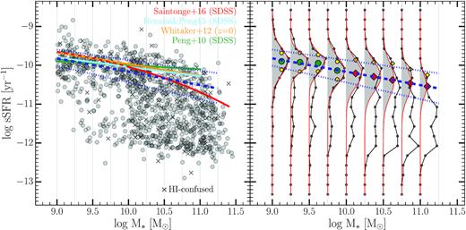
Left-hand panel: sSFR is plotted against stellar mass for our sample (grey circles), including H i-confused galaxies (grey crosses). Blue thick dashed and dotted lines show our SFMS relation and its 1σ scatter, and solid coloured lines show SFMS relations from other groups. Right-hand panel: a visual summary of our SFMS fitting method. Within each stellar mass bin, black lines and points show the sSFR distributions. Grey histograms show the best-fitting Gaussians in each bin. The four green dots show the modes of the unconstrained Gaussian fits at low masses, and the red diamonds show the extrapolation to higher stellar mass. The yellow symbols show the best-fitting 1σ widths in each bin. Our best-fitting SFMS relation (±1σ) is shown as a blue dashed (dotted) line(s).
Other determinations of the SFMS are also shown in the left-hand panel of Fig. 1 and are broadly consistent with ours, although some divergence is seen at higher masses where the SFMS becomes less populated. Each SFMS comes from a different sample of galaxies and uses a different SFR indicator (or indicators), different definitions of star-forming galaxies, and different fitting methods. While all formulations are similar, we adopt the xGASS SFMS for consistency with our previous work.
2.2 Cold gas fraction relations of SFMS galaxies

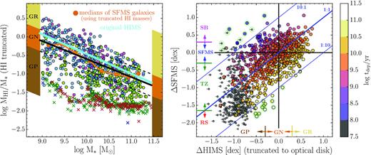
Top two panels: sSFR versus M* is colour coded by position above/on/below the SFMS, with shapes based on their H i (left-hand panel, circles) or CO (right-hand panel, squares) detection status, where crosses indicate non-detections. Galaxies with potentially confused H i observations are not included. Black lines show the xGASS SFMS with ±0.3 dex dashed lines and the threshold of the RS. Bottom two panels: H i and H2 gas fractions use the same colours and shapes as the top panels. The large orange points show median H i and H2 gas fractions of galaxies from the SFMS in bins of stellar mass, black lines show linear fits to those averages, and dashed lines show ±0.3 and ±0.2 dex for H i and H2 gas fractions, respectively.
Since galaxies in the SFMS do not correspond to a similarly tight sequence in either the H i or H2 gas fraction relations, we do not fit Gaussians to determine a width. Instead, we adopt widths of 0.3 dex (0.2 dex) to separate galaxy populations that have |${M}_{\rm H\,{{\small I}}}\, ({M}_{\rm {\rm H}_2})$| values which are similar to the expectation from the simple scaling relation; these widths correspond to the 1σ standard deviations of the SFMS population which is detected in each panel. The bottom two panels of Fig. 2 show these regions of parameter space. Note that in this work we consistently treat the H i and molecular gas masses separately. The gas fraction relations of the total (H i + molecular) gas would be qualitatively similar to the H i relations as the gas reservoirs of the SFMS and TZ galaxies are dominated by the H i component. For a detailed analysis and discussion of scaling relations based on a combined total cold gas mass, see section 4.2 of Catinella et al. (2018).
3 COLD GAS ABOVE/BELOW THE SFMS
Fig. 2 demonstrates the complexity of the correspondence between star formation and cold gas content. Galaxies are colour coded based on their ΔSFMS from the sSFR–M* plot (top two panels). Those within ±0.3 dex (approximately 1σ) of the SFMS are shown in blue, and those with higher sSFR are referred to as starbursts (SB) and shown in magenta. The Red Sequence (RS) is typically dominant below sSFR < −11.8 yr−1 (Salim 2014), which corresponds to ΔSFMS < −1.55 dex for our SFMS, and is shown in red. Between the RS and the SFMS is the transition zone (TZ), shown in green. The precise threshold between the TZ and the RS is somewhat arbitrary; we adopt ΔSFMS = −1.55 dex since below that point only ∼10 per cent (0 per cent) of the galaxies are detected in H i (CO). As we are interested in the cold gas properties of TZ galaxies, this RS definition makes our TZ population more meaningful. Our main conclusions would remain unchanged if we adopted variations on this threshold between the TZ and the RS.
On the top left panel of Fig. 2, filled circles denote galaxies which have been detected in H i, while coloured crosses show sources which do not have H i detections (although still have valid sSFR measurements). The top right panel of Fig. 2 shows the same for molecular gas (CO) observations: filled squares show sources with molecular gas detections, while coloured crosses denote those which have been observed but not detected (again, these are valid sSFR measurements).
The bottom two panels of Fig. 2 show the H i and H2 gas fraction scaling relations, using the ΔSFMS-selected colour scheme. The bottom left panel plots the H i gas fraction scaling relation, with coloured circles showing H i detected galaxies and coloured crosses at the upper limits of non-detections. The bottom right panel plots the H2 gas fraction scaling relation, with coloured squares showing detections and coloured crosses at the upper limits of non-detections. Analogously to the SFMS, here we show the GFMS relation (i.e. fitting the gas fraction scaling relation in H i and H2 for SFMS galaxies only), and identify galaxies within ±0.3 dex (0.2 dex for H2) as gas normal (GN). These widths correspond to 1σ standard deviations of the gas fraction distributions of the SFMS population. Galaxies above this sequence are considered gas rich (GR) and below are gas poor (GP).
There is a general correspondence between these two relations in that the majority of galaxies above the SFMS are also above the GFMS (as was also shown in Saintonge et al. 2016), but there is substantial scatter, especially in the H i relations. In particular, a significant number of TZ galaxies below the SFMS have H i gas fractions which are consistent with (GN) or even above (GR) that of SFMS galaxies. Before discussing specific trends, we first quantify the strength of this correspondence between ΔSFMS and ΔHIMS.
3.1 Correspondence between ΔSFMS and ΔHIMS
First we consider the ΔSFMS populations (SB, SFMS, TZ, and RS) and plot the distribution of ΔHIMS for each in the top left panel of Fig. 3. We include galaxies with H i detections in the solid histogram (for which statistics are computed) and show the upper limits of non-detections as dotted histograms for reference. These populations all have broad distributions of H i gas fractions with 1σ widths of ∼0.4 dex. The average ΔHIMS of the SB, SFMS, and TZ populations varies by only 0.15–0.3 dex, so there is significant overlap between galaxies above, on, and below the SFMS.
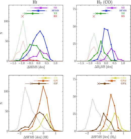
Top panels: histograms of ΔHIMS and ΔH2MS for galaxies selected by ΔSFMS. Bottom panels: histograms of ΔSFMS for galaxies selected by ΔHIMS and ΔH2MS. Galaxies which are detected in each population are shown as solid lines, medians as large solid points, thick lines show ±1 standard deviations, and thin lines show the 5th and 95th percentiles of each population (detections only). Non-detections in each population are shown as dotted histograms. Coloured crosses indicate the medians of the full samples in each population, including both detections and upper limits of non-detections.
Likewise the top right panel of Fig. 3 shows theΔH2MS distributions for the molecular gas of the same populations. Here the distributions are much tighter (∼0.25 dex) but their averages are separated by similar amounts (0.2–0.3 dex). As was visually apparent in Fig. 2, there is a tighter correspondence when comparing SFR with M|$_{{\textrm {H}}_2}$| than with M|$_{\rm{H}\,{{\small I}}}$|. As noted in Catinella et al. (2018), galaxies in the SFMS have a narrower range of M|$_{{\textrm H}_2}$| gas fractions, whereas the M|$_\rm{H\,{{\small I}}}$| gas fraction can change by two orders of magnitude. The averages and standard deviations of the ΔHIMS and ΔH2MS distributions are quantified in Table 1.
Population sizes (detections and non-detections), averages, and standard deviations (of detections only), and medians (of detections and non-detections) are given for each selection. <ΔHIMS> and <ΔH2MS> are computed for SFMS-selected populations (SB, SFMS, TZ, RS), and <ΔSFMS> is computed for ΔHIMS- and ΔH2MS-selected populations (GR, GN, GP). When fewer than half of the galaxies in a selected population are detected, medians are not computed.
| H i | H2 | |||||||
|---|---|---|---|---|---|---|---|---|
| ΔSFMS | Nd | (Nnd) | <ΔHIMS> | <ΔHIMS>med | Nd | (Nnd) | <ΔH2MS> | <ΔH2MS>med |
| SB | 107 | (3) | +0.10 (0.35) | +0.13 | 52 | (4) | +0.33 (0.24) | −0.20 |
| SFMS | 349 | (20) | −0.03 (0.36) | −0.02 | 136 | (14) | +0.01 (0.20) | −0.02 |
| TZ | 211 | (246) | −0.33 (0.36) | – | 73 | (105) | −0.30 (0.27) | – |
| RS | 11 | (117) | −0.53 (0.28) | – | 0 | (50) | – | – |
| ΔHIMS | Nd | (Nnd) | <ΔSFMS> | <ΔSFMS>med | Nd | (Nnd) | <ΔSFMS> | <ΔSFMS>med |
| GR(2) | 106 | (0) | +0.15 (0.31) | +0.17 | 65 | (4) | +0.33 (0.30) | +0.36 |
| GN(2) | 350 | (0) | −0.08 (0.41) | −0.03 | 126 | (14) | −0.00 (0.27) | +0.03 |
| GP(2) | 222 | (386) | −0.43 (0.55) | −1.02 | 70 | (155) | −0.51 (0.35) | – |
Carrying out general correspondence between these two a similar selection process in the reverse direction, the bottom left panel of Fig. 3 shows the ΔSFMS distributions of the GFMS-selected populations (GR, GN, GP). Here again the correlation between H i content and SFR is weak, as all three distributions have significant overlap. The most gas-rich galaxies have the narrowest distribution of ΔSFMS, suggesting that elevated star formation is very likely given a rich supply of atomic gas. However, even this gas-rich population has a tail that extends to −1σSF below the SFMS.
The bottom right panel of Fig. 3 shows the ΔSFMS distributions for the GF2MS-selected populations (GR2, GN2, GP2). These distributions are again tighter than those selected by ΔHIMS, but not as tight as those in the top right panel. This suggests that the correlation from SFR to H2 content is stronger than the correlation from H2 content to SFR. The averages and standard deviations of these ΔSFMS distributions for the populations selected by H i and H2 gas fractions are also given in Table 1.
3.2 Depletion times and the SFMS
Galaxies above the SFMS (with higher SFR) are likely to deplete their cold gas reservoirs more quickly than those below the SFMS (with lower SFR). However, given the wide scatter in gas properties below the SFMS, we next compute depletion times (tdep = Mgas/SFR) for each galaxy using their H i and H2 masses. These depletion times represent the time-scale for total gas consumption when assuming a very simplistic constant SFR and no gas recycling. Some previous work has suggested that star-forming galaxies are re-fuelled on ∼Gyr time-scales on average, which complicates this simple picture (Kannappan et al. 2013). Furthermore, the physical extents of the H i and molecular gas distributions are likely quite different, and our unresolved observations cannot distinguish between gas in the far outskirts (which must first migrate inwards before it can play a role in star formation) and gas in the inner regions (which may be consumed on shorter time-scales). Nonetheless, the H i and H2 depletion times are useful to estimate the evolutionary potential of galaxies on and outside the SFMS. Previous observations of H2 depletion time have shown a near constant value (0.7 Gyr) in SFMS galaxies across cosmic time (Tacconi et al. 2013), while others show a dependence on sSFR such that more star-forming galaxies have shorter depletion times (Saintonge et al. 2011, 2016).
In this work we use the depletion time as a crude estimate of the evolutionary pace of a galaxy: those with shorter depletion times are likely to be more rapidly evolving and transforming (i.e. consuming a significant fraction of their gas supply on short time-scales), while those with longer depletion times are evolving more slowly. The left-hand panel of Fig. 4 shows histograms of H i depletion times for each ΔSFMS population (SB, SFMS, TZ, RS) using the same colour-coding as previous figures. Within each population, average H i depletion times based on H i detections are shown with large symbols with 1σ error bars as well as 5th and 95th percentiles. Crosses show medians within each population, using both detections and non-detections.
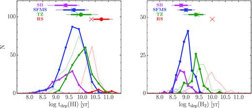
H i (left) and H2 (right) depletion times for SB (magenta), SFMS (blue), and TZ (green) galaxy populations with gas detections (non-detections are shown as dotted lines). Medians of the detections in each population are shown as large symbols with thick 1σ error bars and thin lines extending to the 5th and 95th percentiles. Coloured crosses show the medians of the full samples in each population, including both detections and upper limits of non-detections.
Galaxies in the xGASS SFMS (in blue in Fig. 4) span a wide range of H i depletion times varying from 0.8 to 40 Gyr. The average H i depletion time is ∼6.2 Gyr with a scatter of 0.6 dex. In the TZ below the SFMS (plotted in green), galaxies span a similar dynamic range of H i depletion times (from 7–70 Gyr, one order of magnitude), with an average of ∼9.7 Gyr. Above the SFMS, SB galaxies (plotted in magenta) again have a larger dynamic range (1.3–130 Gyr) but a shorter average H i depletion time of ∼2.9 Gyr.
The right-hand panel of Fig. 4 shows histograms of H2 depletion times for the same ΔSFMS populations with the same colour-coding. Within the SFMS, the dynamic range of H2 depletion times is similar that in H i, but offset to shorter times, as shown in the right-hand panel of Fig. 4, spanning only 0.3–3 Gyr, with an average of ∼1.1 Gyr and a scatter of 0.49 dex. As with H i, SB galaxies have shorter H2 depletion times (average of 0.8 Gyr), and galaxies in the TZ have longer H2 depletion times (average of 2.8 Gyr).
Combining all of the cold gas and SFR information, we plot ΔSFMS versus ΔHIMS and ΔH2MS in Fig. 5, in a similar way to fig. 11 of Schiminovich et al. (2010). These plots show the general trend for galaxies above (below) the average H i and H2 scaling relations to have positive (negative) ΔSFMS, and they also demonstrate the significant amount of scatter in this trend. Points in Fig. 5 are colour coded by their gas depletion time, and SFMS- and GFMS-selected populations are labelled along the axes.
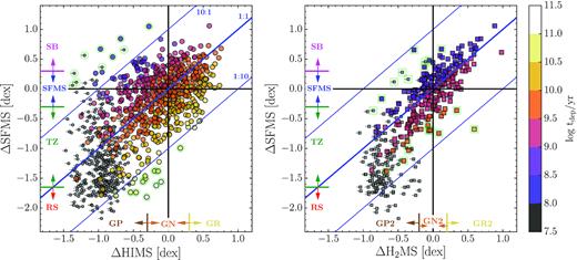
ΔSFMS is plotted versus ΔHIMS and ΔH2MS, colour coded by depletion time (using circles for M|$_{\rm{H}{{{\small I}}}}$| and squares for M|$_{{\textrm {H}}_2}$|, respectively). Regions of ΔSFMS and ΔHIMS populations are indicated along each axis. Galaxies with H i/CO non-detections are shown as small grey symbols at their upper limit ΔHIMS with short lines extending towards permitted gas fractions. Diagonal lines show 1:1, 10:1, and 1:10 ratios. Note that the depletion time at the origin is different between the two panels (∼109.6 yr in H i, and ∼109.0 yr in M|$_{{\textrm H}_2}$|). The 10 longest and 10 shortest depletion time galaxies in each panel are surrounded by light green haloes and are discussed further in Section 3.3 (see also Fig. 6).
3.3 Galaxies with extreme depletion times
Given the broad correspondence between ΔHIMS and ΔSFMS in Fig. 5, we take a closer look at those which deviate from this general trend. That is, we examine galaxies with the most extreme depletion times to explore what factors may contribute to their departure from the main relation. It is important to note that a galaxy’s SFR is expected to stochastically fluctuate, so a galaxy which currently exhibits an extreme depletion time may be experiencing a brief fluctuation in its SFR (increase or decrease) and not a permanent transition. These fluctuations can have particularly strong effects on the lowest mass galaxies in our sample.
First, we select the 10 galaxies with the shortest H i depletion times and indicate their locations with light green haloes in the top left corner of the left-hand panel of Fig. 5. We include H i non-detections in this selection, as these translate directly to upper limits on depletion times, and note that these short H i depletion time galaxies are all in the SFMS or SB populations. SDSS thumbnail images are shown for these galaxies in the top row of Fig. 6. We also include the environmental identity for each galaxy from the Yang et al. (2007) DR7 group catalog (discussed further in Section 4), and do not include the 16 galaxies from our sample which lack environmental identities largely due to their proximity to survey edges.
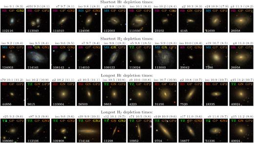
SDSS thumbnail images (80 arcsec on a side) are shown of galaxies with the extreme H i and H2 depletion times, ordered by increasing stellar mass from left to right. Above each thumbnail is its environmental identity (isolated central or satellite/group central with the number of group members), the logarithm of its stellar mass (in solar units) and the logarithm of its depletion time (in years and in parentheses). Overlaid on each image are its ΔSFMS, ΔHIMS, and ΔH2MS categories, and its xGASS ID.
These short H i depletion time galaxies have (potentially completely) diminished gas reservoirs but unexpectedly strong star formation. As seen in their SDSS thumbnails, at least half show strong bars or ring features, suggesting they may have more efficient star formation than an otherwise similar galaxy without a bar. These short depletion time galaxies are likely to be the most rapidly evolving systems. Without an additional supply of gas, their SFR will soon decrease and they may drop back down to (or even below) the 1:1 line in Fig. 5.
Similarly, we select the 10 galaxies with the shortest H2 depletion times and indicate their positions in the right-hand panel of Fig. 5. These are found largely in the SB and SFMS, but one is in the TZ. Thumbnails from SDSS of this population are shown in the second row of Fig. 6, and they have similar morphologies to the galaxies with the longest H i depletion times. Only two galaxies (xGASS 114 010 and 26 958) are common to both categories: xGASS 114 010 has a strong bulge and is a satellite in a group of N = 7; xGASS 26 985 is a central in a group of N = 4 and shows a dramatic system of shells/rings suggesting a recent interaction.
At the other extreme, we consider the 10 galaxies with the longest H i depletion times, which are also indicated with light green haloes in the bottom right corner of the left-hand panel of Fig. 5, and their thumbnails are shown in the third row of Fig. 6. Here we require H i detections to compute meaningful depletion times, as upper limits on H i masses also yield upper limits on H i depletion times. Without a detection, the true depletion time could be significantly smaller and much less extreme. This population of long H i depletion time galaxies (with good H i detections) is found in the TZ and RS.
These galaxies have a significantly larger H i reservoir than expected from their SFR, so the atomic gas may be inaccessible, lingering below a density threshold, or experiencing too much shear or dispersion to trigger star formation. This inaccessibility could mean that the gas has arrived with high angular momentum from a minor merger, so has not yet collapsed enough to form a proportionate amount of star formation. Our H i observations are unresolved, so the neutral gas has not been localized within the galaxy, and may be significantly more extended than the stellar components (perhaps analogously to the sample identified and observed by Geréb et al. 2016, 2018), but interferometric observations of their H i would be required to confirm this scenario. These galaxies are all fairly massive (M* ≥ 1010 M⊙) and have strong bulges, but at least four show (hints of) discs as well. Galaxies with substantial H i reservoirs like these are candidates for possible rejuvenation (i.e. a return to the SFMS) if they are able to access their full gas supply for star formation. At their current star formation rates, these long-depletion-time galaxies are some of the most slowly evolving galaxies. They are unlikely to move significantly within Fig. 5 and represent a moderately static gas-rich population.
Analogously, the longest H2 depletion time population is selected in the same way and displayed in the 4th row of Fig. 6. Note in particular that GASS 40024 has both an extreme H i depletion time and an extreme H2 depletion time, and is a satellite in a group of N = 15 galaxies. This long H2 depletion time population also includes galaxies at lower masses and are all found in the TZ. Here the number of edge-on galaxies with visible absorption from dust lanes suggests that some members of this population may have underestimated SFRs. Our SFR is based on both the direct UV emission from young stars and the re-processed IR emission from dust absorption, but the edge-on systems with strongly visible dust lanes may be more extincted than our SFR calibration assumes. If the SFR estimates of edge-on galaxies are underestimated, then their depletion times will be artificially increased.
3.4 Predicting gas location from scaling relations and predicting H i masses within optical disc
One might consider the role that the spatial location of cold gas within the galaxies in our sample plays in determining their star formation histories and depletion times. For example, gas-rich TZ galaxies may remain gas-rich (with long depletion times) if their remaining gas is largely located in their outskirts and only slowly migrates to the inner regions to participate in active star formation. Accounting for potential differences in H i and stellar distributions would require resolved H i observations, but even without those we can employ simple scaling relations to predict the amount of H i mass contained within the optical disc. In this way we can estimate the depletion time considering only the gas which is predicted to be contained within the optical disc
We use the H i size–mass relation from Wang et al. (2016) to predict an H i size using only the H i mass of each galaxy in our sample. We also adopt a simple exponential profile for the radial H i mass distribution. Using the 90 per cent Petrosian radius from the SDSS r image, we integrate the exponential profile within this truncation radius to determine the H i mass contained within the optical disc. This is a simple approach and relies on the assumption that these galaxies all follow the H i size–mass relation and all have the same profile shape. Still, these simple truncated H i masses will give an indication of the potential impact that the spatial distribution of H i could have on our results.
The left-hand panel of Fig. 7 shows an updated version of the H i gas fraction scaling relation, originally presented in Fig. 2, but now using the H i masses truncated within the optical disc. As expected, this overall reduction in H i masses results in a slightly lower median relation than with the full H i masses, with a very weak change in slope. The right-hand panel of Fig. 7 plots ΔSFMS versus ΔHIMS for these truncated H i masses. When compared with the left-hand panel of Fig. 5, no significant differences are observed. Since the truncated H i masses are always smaller than the total H i masses, there is again a systematic shift towards lower values of ΔHIMS. This does not indicate that the spatial distribution of the gas is unimportant, but rather suggests that there are no significant effects revealed by this truncation of an assumed H i profile within the optical disc. Resolved observations of the H i gas would be required to advance this question further.
Left-hand panel: H i gas-fraction scaling relation is plotted using H masses truncated within the optical disc, as described in Section 3.4. Orange points and black line indicate the median relation for SFMS galaxies, compared to the original relation from Fig. 2 shown in cyan. Right-hand panel: truncated H i masses are used to reproduce the left-hand panel of Fig. 5, using the updated HIMS from the left-hand panel. While subtle, there is a small systematic offset towards lower values of ΔHIMS, but the same appearance overall.
4 UN-QUENCHED GALAXY POPULATIONS BELOW THE SFMS
Using the populations described in Fig. 5, we next focus on the galaxies found in the TZ between the SFMS and the RS. Here we refer to ‘quenched’ galaxies as those with SFR measurements low enough to be consistent with no active star formation and such small cold gas reservoirs as to be undetectable. We will consider the types of evolutionary scenarios and pathways that TZ galaxies may follow. First, however, it is important to note that galaxies in the TZ with cold gas detections have on average ∼0.35 dex longer H i and H2 depletion times than those in the SFMS. This is visible in Fig. 4, which also makes clear the significant overlap between both populations. Of the ∼400 galaxies in the TZ, ∼50 per cent are detected in H i and 40 per cent of these H i detections are comparably or more gas-rich than typical SFMS galaxies (i.e. are GN or GR). This suggests that a significant fraction of the TZ galaxies are not actively quenching or rapidly evolving towards the RS. The remaining TZ galaxies without H i detections may be a more rapidly evolving/quenching population, but the TZ galaxies with H i detections can sustain their current SFR longer than galaxies currently in the SFMS!
While all galaxies in the TZ could naively be considered ‘quenched’ based on their sSFR alone, we are interested in separating the TZ into meaningful populations that may evolve on different pathways. We begin by separating TZ galaxies by their environmental identity as satellite or central galaxies, since we expect these populations to evolve through different mechanisms. We use the SDSS DR7 group catalog of Yang et al. (2007) to divide our sample into satellite members of groups, central members of groups, and isolated central galaxies, and we first consider the satellite galaxy population.
4.1 Satellite galaxies in the TZ
There are 160 satellite galaxies from xGASS in the TZ, of which 67 have H i detections. The left-hand panel of Fig. 8 shows the ΔHIMS versus ΔSFMS plot for all satellites, with medians plotted in bins of ΔSFMS. Compared with central galaxies (in groups and in isolation), satellites have median ΔHIMS values which are smaller both on and below the SFMS (above the SFMS, the central and satellite populations are indistinguishable). The median offset in ΔHIMS between the H i-detected TZ satellite and central galaxies is ∼0.47 dex, which is larger than the analogous offset in the SFMS (∼0.10 dex). Quantitatively, the distributions of ΔHIMS for H i-detected central and satellite galaxies in the TZ are different at the 98.8 per cent level (p = 0.012) using a two-tailed p-value KS test. This reduced gas content of satellite galaxies is broadly consistent with environmental stripping/quenching scenarios, where a reduction of gas content precedes a decrease in star formation activity.
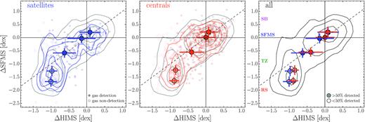
Each panel shows ΔHIMS versus ΔSFMS, for satellite galaxies (left-hand panel, blue), central galaxies (middle panel, red), and the total population (right-hand panel). Contours and medians in bins of ΔSFMS are shown for each population, with 25th/75th percentile error bars; the unity line is shown with dashes. Large median points are filled if more than half are detected in H i. Satellite galaxies in the TZ are offset to lower median ΔHIMS than central galaxies; a KS test on these two distributions produces p = 0.012 implying they are significantly different from each other.
While the ΔHIMS distributions of central and satellite galaxies in the TZ show statistically significant differences, it is difficult to physically interpret any differences in ΔHIMS alone since it implicitly includes a dependence on M* (present in the H i gas fraction shown in Fig. 2). In order to quantify this apparent quenching of satellite galaxies in a more physical sense, we instead consider the distributions of their H i depletion times (using only galaxies with H i detections). In the TZ, a KS test of the distributions of H i depletion times for central and satellite galaxies produces a two-sided p-value of p = 0.13, implying these samples are only weakly distinct from each other.
To dig deeper into the significant trends identified in ΔHIMS, Fig. 9 shows the H i depletion times for TZ galaxies now separated into three bins of stellar mass. In all bins, the distributions of H i depletion times for satellite and central TZ galaxies have similar widths of ∼0.4 dex. In the lowest mass bin (with the highest H i detection fraction), satellite TZ galaxies have median H i depletion times of 109.6 yr, while central TZ galaxies have a median of 109.8 yr. This difference is not very large and a KS test on these two distributions of depletion times yields only p = 0.26. The same galaxies have ΔHIMS distributions which are different by p = 0.07, which is somewhat more significant. The middle and high mass bins show even smaller differences between TZ satellites and centrals, so this trend appears to be driven by the galaxies at lower mass.
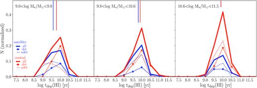
Normalized histograms of H i depletion time for TZ galaxies which are centrals (red) and satellites (blue), divided into three bins of stellar mass. Thick lines show histograms of all of the (H i) detected and non-detected galaxies, thin lines show only detections, and dotted lines show only non-detections. Vertical lines are drawn at the median depletion time for each population (including detections and non-detections). In the lowest mass bin the satellites (N = 12) have shorter depletion times than centrals (N = 25) and a KS test between these two distributions gives p = 0.26 which is a weak difference. The middle and high mass bins show less significant differences in their H i depletion times.
The reason why H i depletion times show less of a difference than ΔHIMS is most likely because changes in SFR and H i content cancel each other and/or increase the scatter. As shown in Fig. 8, central and satellite galaxies are different at nearly fixed ΔSFMS, but their difference relative to the diagonal dashed line (i.e. constant depletion time) is inevitably less significant.
While this difference in H i depletion times is small (p = 0.012), a systematically lower H i content in satellites at fixed star formation rate (i.e. shorter depletion times) than centrals is in line with a simple evolutionary picture where satellite quenching is driven primarily by gas stripping. In this scenario, satellite galaxies in the TZ (especially those at low mass) have had their gas reservoirs reduced more rapidly and their star formation is still declining to match. This points towards active stripping of gas being more important in the evolution of satellites than central galaxies, though the large scatter may indicate multiple evolutionary paths also for the satellite population.
4.2 Central galaxies in the TZ
There are 297 central galaxies from xGASS in the TZ, of which 158 have H i detections. Galaxies in the TZ span a similarly wide range of H i depletion times compared with those in the SFMS or above it. As discussed in Section 4.1, the smaller gas reservoirs of satellite galaxies in the TZ is consistent with a picture of environmental effects driving them into the TZ. In this section we now focus on the central galaxies, which we expect to be less affected by their environment. Here we combine all central galaxies (those in groups/clusters and those in isolation) into a single sample for better statistics. This yields a sample of 297 central galaxies in the TZ. We also carry out the following analysis on subsets of isolated only and group central galaxies only, and find no significant differences from the results discussed below.
To explore this population, we divide the central galaxies in the TZ into three roughly equal-sized populations based on their (H i) depletion times. ‘Typical’ centrals have tdep between ∼5 and ∼11 Gyr, and represent the middle trintile of the distribution. Those with longer depletion times are considered ‘slow,’ and shorter are considered ‘fast.’ We also note that this population of central TZ galaxies with ‘typical’ H i depletion times is found along the 1:1 line shown in Fig. 5, the ‘fast’ are found above the unity line, and the ‘slow’ below.
We test for possible trends with a few fundamental observed properties of the TZ centrals in these ‘fast,’ ‘typical,’ and ‘slow’ populations. With regard to their environment, we consider the density of nearby neighbours and their halo mass as given by abundance matching in the group catalogue of Yang et al. (2007). When using the density of galaxies per projected Mpc2 within the seventh nearest neighbour, we find no significant difference between these three populations of TZ centrals. Similarly, no trends are found with the halo masses. Both of these results suggest that the gas content in TZ centrals is not strongly affected by their environment, and that this population may evolve through a variety of channels.
Looking internally, we also look for trends with average stellar surface density, μ*, defined as M*/(2πR|$_{50,z}^2$|), where the z filter half-light radius R50,z is measured in kpc. All three populations of TZ centrals have larger average values than non-TZ central galaxies, which is consistent with the typical morphologies seen below the SFMS (e.g. Salim et al. 2007). However, we find no significant trends as a function of μ*. This further shows the diversity and scatter within this population.
The only meaningful trend we identify appears when considering the ratio of UV and optical size of the TZ centrals. We use the ratio of the half-light radius measured in NUV to the half-light radius in the optical r filter, including only ∼75 per cent of galaxies that have been resolved in the GALEX images (i.e. r > 5 arcsec). Here the three TZ central populations show a consistent trend: those with the longest H i depletion times also have the highest average UV-to-optical size ratios, and the smallest H i depletion times have the smallest UV-to-optical size ratios.
Fig. 10 shows this UV-to-optical size ratio versus stellar mass for central galaxies in our sample. Those in the TZ are plotted in colours corresponding to their depletion time; all non-TZ central galaxies are shown as grey dots. There is a weak trend evident with stellar mass such that more massive galaxies have larger UV-to-optical size ratio. Additionally, most of the central galaxies with the largest UV-to-optical size ratios are found in the TZ. However, most intriguing is the trend amongst the TZ galaxies such that those with longer depletion time (i.e. ‘slow’) have larger typical UV-to-optical size ratios. This is most clearly visible in the stellar mass bin centred around 1010.5 M⊙, where there are more galaxies of each population included in the median. For a visual example, Fig. 11 shows sample images of TZ galaxies in the ‘slow’ (with large UV-to-optical size ratio) and ‘fast’ (with small UV-to-optical size ratio) subsets. In particular, GASS 3505 was identified by Geréb et al. (2016) as a prototypical example of an ‘H i-excess’ galaxy – a population which has large H i reservoirs but insignificant amounts of star formation (Geréb et al. 2018).
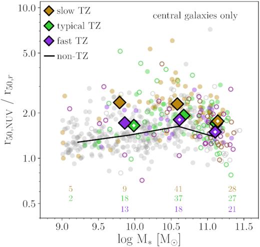
Only central galaxies are plotted, using different colours for those in the TZ with short H i depletion times (fast, purple), average depletion times (typical, green), and long (slow, brown). Grey symbols indicate central galaxies outside of the TZ. Solid symbols denote H i detections, and open show upper limits of non-detections. Large diamonds show medians (including detections and non-detections) in bins of stellar mass (when fewer than 50 per cent are detected, the diamonds are open). Numbers at the bottom indicate how many galaxies are in each binned median. The black line connects medians of the non-TZ central galaxies. TZ central galaxies show a trend with the UV-to-optical size ratio such that those with longer (slower) depletion times have larger ratios.
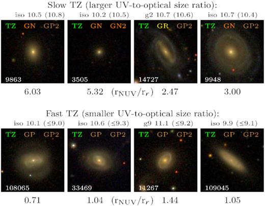
SDSS colour images of example central galaxies from the TZ, selected for their slow (top row) or fast (bottom row) H i depletion times. TZ central galaxies with long depletion times typically show star formation activity in their outskirts and have a larger UV-to-optical size ratio, while those with short depletion times more often have central star formation and small ratios of UV-to-optical size. Galaxies are labelled as in Fig. 6, with their environmental identity, stellar mass, and H i depletion time. The UV-to-optical size ratio (rNUV/rr) of each galaxy is listed underneath its thumbnail.
This correlation between depletion time and UV-to-optical size ratio suggests that the star formation in the ‘slow’ TZ galaxies is more radially extended than in typical galaxies. It may mean that the excess H i reservoir is also more spatially extended and inaccessible to star formation. An inaccessible H i reservoir may lead to low star formation efficiency; ∼90 per cent of the ‘slow’ TZ central galaxies have depletion times longer than a Hubble time (and ∼15 per cent are more than twice as long as a Hubble time). Intriguingly, for the ∼40 per cent of TZ galaxies with molecular observations there is no correlation between the molecular and atomic gas depletion times, and all three populations have average molecular gas depletion times of ∼3 Gyr. The apparent tightness of the relation between ΔSFMS and ΔH2MS (shown in the right-hand panel of Fig. 5) supports the fact that SFR proceeds whenever molecular gas is available (see e.g. Schruba et al. 2011); the inaccessible H i may be in an extended low-density configuration which prevents it from converting to molecular gas and forming stars. These ‘slow’ galaxies may still be forming stars (albeit slowly) long after the galaxies in the SFMS have exhausted their gas, fully quenched, and joined the RS.
5 DISCUSSION
Galaxies in the TZ below the SFMS do not appear to make up a unified population, as many external and internal mechanisms can drive galaxies into (or out of) this so-called ‘green valley.’ Compared to SFMS galaxies, TZ galaxies have a similar range of H i gas fractions and longer depletion times, and are found across all environments, providing a large range of available evolutionary pathways.
When considering the role of external environmental effects, we have demonstrated that satellite galaxies with low ΔHIMS (see Section 4.1) may be examples of some TZ galaxies which have experienced a cessation of star formation following the ram pressure stripping of their gas by a cluster environment. Vulcani et al. (2015) also find a weak connection between environment and quenched galaxies, but also identify a population of galaxies with intermediate optical colours which are not rapidly quenched but instead are experiencing declining SFH over long time-scales (>1 Gyr).
Our sample of TZ galaxies have average H i depletion times of ∼10 Gyr (see Section 3.2), suggesting that this population is not rapidly moving towards the RS through secular evolution alone. This population of long depletion time TZ galaxies is in contrast with the expectations from other studies of the stellar populations of TZ galaxies. For example, while Smethurst et al. (2015) find evidence for multiple evolutionary paths through the TZ, their scenario only requires 1–1.5 Gyr for a galaxy to transit the TZ. Similarly, using the EAGLE hydrodynamic simulation, Trayford et al. (2016) selected TZ galaxies based on their u–r colours and found that they spend less than 2 Gyr transiting between the SFMS and RS. This apparently rapid quenching and disagreement with our findings is largely a result of selecting TZ galaxies (and determining their SFRs) based only on optical colours. As effectively demonstrated by fig. 4 in Salim (2014), TZ and RS galaxies have indistinguishable optical colours and it is difficult to make meaningful distinctions between these populations without UV observations.
Another formation scenario for TZ galaxies is that they have depleted their gas reservoirs and are fading on to the RS. The results of Schawinski et al. (2014) support the idea of multiple evolutionary pathways through the TZ, but argue that the star formation rates are responding to changes in their (un-observed) gas supplies. They claim that late-type TZ galaxies have had their cosmic gas supply cut off, and that early-type TZ galaxies have recently experienced a rapid quenching as a result of the destruction of their gas supply by a possible major merger. (We found no dependence of any of our relationships on μ*, a proxy for morphology, as discussed in Section 4.2.) Bremer et al. (2018) also argue that an insufficient gas supply is responsible for galaxies rapidly (∼1–2 Gyr) evolving through the TZ. While our work does confirm that TZ galaxies have lower average H i gas fractions than those in the SFMS, the range of gas fractions is actually larger in the TZ, and their long gas depletion times (∼10 Gyr on average) are not consistent with rapid quenching scenarios.
When selecting TZ galaxies based on UV and optical observations, others have also found TZ galaxies still forming stars at a sustainable rate. In particular, Fang et al. (2012) identified a population of ‘extended star-forming early-type galaxies’ (ESF-ETGs) which were selected using their global photometry on a UV-optical colour–magnitude diagram. While consistent with TZ in a global sense, these ESF-ETGs look red and morphologically early type at their centres but their outskirts are blue and show UV emission from young stars. Fang et al. (2012) suggest that this population of TZ galaxies may persist for several Gyrs before fading into the RS, consistent with our results.
Studies of the gas content in star-forming galaxies at higher redshifts have identified similar trends to those discussed in this work. Notably, the Plateau de Bure high-z Blue Sequence Survey (PHIBSS, Genzel et al. 2015; Tacconi et al. 2018) observed molecular gas masses in 32 galaxies at z = 1.2 and 2.2 with stellar masses above 1010.4 M⊙, and found that their molecular gas fraction generally decreases with time and that their molecular gas depletion times increase further below the SFMS, independent of stellar mass. More recently, the low-redshift (z = 0.5–0.8) sample of PHIBSS2 galaxies between 1010 < M*/M⊙ < 1011.4 showed that this trend for molecular gas depletion time to increase below the SFMS also continues towards lower redshifts (Freundlich et al. 2019). These relations are also consistent with the results of Saintonge et al. (2012), Saintonge et al. (2017), who used the COLD GASS and xCOLD GASS samples (which are also used in this work and consist of direct CO observations rather than indirect gas indicators used at higher redshifts) to determine that the molecular gas depletion time increases by ∼0.3 dex between galaxies in the SFMS and the TZ. Our findings that local galaxies below the SFMS have longer H i depletion times fits naturally into this picture, and we have explored a few of the features and mechanisms at play in this evolution.
Many evolutionary paths lead through the TZ, and today’s TZ galaxies appear to be able to evolve in almost any direction in Fig. 5. As a population, our TZ galaxies do not appear to represent an intermediate stage between the SFMS and the RS, but rather are a diverse population, as seen most clearly through observations of their cold gas content.
6 SUMMARY
In this work we have used the xGASS and xCOLD GASS samples to explore the cold gas properties of galaxies in the TZ below the SFMS. Our main findings are as follows:
Galaxies in the SFMS have large scatter in H i gas fraction scaling relation, but tighter in H2. There is no corresponding ‘H i main sequence’ of galaxies in the SFMS.
Compared with galaxies in the SFMS, the H i depletion times of galaxies in the TZ are longer, suggesting it is not a uniformly rapidly quenching/evolving population, and evolves more slowly than the SFMS.
Satellite galaxies in the TZ show a trend to be more gas poor than TZ centrals, especially in terms of ΔHIMS. This trend is weaker when measured in H i depletion time and appears to originate from the lowest mass galaxies (|${M}_*/\rm {M}_\odot \lt 10^{9.8}$|), which is generally consistent with environmental stripping processes removing the gas.
Central galaxies in the TZ show a trend between their H i depletion time and UV-to-optical size ratios, suggesting that they have remained gas rich as a result of inefficient star formation proceeding slowly in their outer discs. Visual inspection of this population shows a variety of disc galaxies with strong bulges and blue outer discs.
In order to further improve our understanding of the evolutionary pathways available to galaxies in the TZ, we need enhanced spatial and temporal resolution of their star formation activity. Given the spatial distributions of UV emission discussed in Section 4.2, follow-up imaging in H α or UV would allow us to better understand if star formation in TZ galaxies is proceeding in different ways than in the SFMS. Re-constructing the star formation histories of TZ galaxies would be invaluable in determining whether they have been a long-lived TZ population or have recently experienced a decline in SFR.
Better separating the mass contributions from the disc (star-forming, associated with gas reservoir) and the bulge (passive) in the xGASS galaxies would also provide a clearer picture of the evolutionary context of the TZ (e.g. Cook et al. 2019). Bulge growth can contribute to a galaxy’s decline from the SFMS to the TZ, and in cases where the depletion times of the bulge and disc can be mapped separately (e.g. Lin et al. 2017), it is clear that bulge quenching and disc quenching are important and somewhat independent processes which drive galaxies away from the SFMS. A better separation of bulge and disc masses will help clarify these evolutionary pathways.
ACKNOWLEDGEMENTS
We thank Toby Brown, Katinka Geréb, and Robin Cook for helpful discussions, and the anonymous referee for their careful reading and thoughtful suggestions which have helped improve this work.
SJ, BC, and LC acknowledge support from the Australian Research Council’s Discovery Project funding scheme (DP150101734). Parts of this research were conducted by the Australian Research Council Centre of Excellence for All Sky Astrophysics in 3 Dimensions (ASTRO 3D), through project number CE170100013. LC is the recipient of an Australian Research Council Future Fellowship (FT180100066) funded by the Australian Government.
This research has made use of NASA’s Astrophysics Data System, and also the NASA/IPAC Extragalactic Database (NED), which is operated by the Jet Propulsion Laboratory, California Institute of Technology, under contract with the National Aeronautics and Space Administration. This research has also made extensive use of the amazingly invaluable Tool for OPerations on Catalogues And Tables (TOPCAT,2 Taylor 2005).
Funding for SDSS-III has been provided by the Alfred P. Sloan Foundation, the Participating Institutions, the National Science Foundation, and the U.S. Department of Energy Office of Science. The SDSS-III web site is http://www.sdss3.org/.
SDSS-III is managed by the Astrophysical Research Consortium for the Participating Institutions of the SDSS-III Collaboration including the University of Arizona, the Brazilian Participation Group, Brookhaven National Laboratory, Carnegie Mellon University, University of Florida, the French Participation Group, the German Participation Group, Harvard University, the Instituto de Astrofisica de Canarias, the Michigan State/Notre Dame/JINA Participation Group, Johns Hopkins University, Lawrence Berkeley National Laboratory, Max Planck Institute for Astrophysics, Max Planck Institute for Extraterrestrial Physics, New Mexico State University, New York University, Ohio State University, Pennsylvania State University, University of Portsmouth, Princeton University, the Spanish Participation Group, University of Tokyo, University of Utah, Vanderbilt University, University of Virginia, University of Washington, and Yale University.
Footnotes
http://www.mpa-garching.mpg.de/SDSS/DR7/; we used the improved stellar masses from http://home.strw.leidenuniv.nl/∼jarle/SDSS/
