


ABSTRACT
The time evolution of angular momentum and surface rotation of massive stars are strongly influenced by fossil magnetic fields via magnetic braking. We present a new module containing a simple, comprehensive implementation of such a field at the surface of a massive star within the Modules for Experiments in Stellar Astrophysics (mesa) software instrument. We test two limiting scenarios for magnetic braking: distributing the angular momentum loss throughout the star in the first case, and restricting the angular momentum loss to a surface reservoir in the second case. We perform a systematic investigation of the rotational evolution using a grid of OB star models with surface magnetic fields (M⋆ = 5–60 M⊙, Ω/Ωcrit = 0.2–1.0, Bp = 1–20 kG). We then employ a representative grid of B-type star models (M⋆ = 5, 10, 15 M⊙, Ω/Ωcrit = 0.2, 0.5, 0.8, Bp = 1, 3, 10, 30 kG) to compare to the results of a recent self-consistent analysis of the sample of known magnetic B-type stars. We infer that magnetic massive stars arrive at the zero-age main sequence (ZAMS) with a range of rotation rates, rather than with one common value. In particular, some stars are required to have close-to-critical rotation at the ZAMS. However, magnetic braking yields surface rotation rates converging to a common low value, making it difficult to infer the initial rotation rates of evolved, slowly rotating stars.
1 INTRODUCTION
Magnetic fields are routinely detected in stars across the entire Hertzsprung–Russell diagram (HRD), from early to late evolutionary phases (Donati & Landstreet 2009). Surface magnetic fields are detected in 7 per cent of hot, massive, OB stars (Wade et al. 2014, 2016; Fossati et al. 2015; Martins et al. 2015; Morel et al. 2015; Neiner et al. 2015; Grunhut et al. 2017; Shultz et al. 2018; Petit et al. 2019). Unlike those detected in cool stars, these surface fields are likely not being actively generated by a dynamo mechanism, especially because there is no evidence that extended convection zones1 exist at the surfaces of hot stars. The long-term stability and the large-scale structure of these fields (along with the lack of apparent correlation between the field characteristics and stellar or rotational parameters) suggest that these fields are fossil remnants formed during the earlier history of the star (Cowling 1945; Mestel 1989; Moss 2003; Braithwaite & Spruit 2004; Donati & Landstreet 2009; Neiner et al. 2015). The typical global configuration is approximately a dipole, inclined with respect to the rotation axis, and the polar field strength is usually of the order of a few kG.
Surface magnetic fields have a complex interaction with stellar winds, confining the wind material along closed magnetic field lines (Babel & Montmerle 1997; ud-Doula & Owocki 2002; Owocki & ud-Doula 2004; Townsend & Owocki 2005; Bard & Townsend 2016). This interaction leads to two dynamical effects that have a considerable impact over evolutionary time-scales: mass-loss quenching, which reduces the effective mass-loss rate of the star, and magnetic braking, which reduces the angular momentum of the star.
Early analytic studies described the role of the magnetized solar wind to explain the slow rotation of the Sun (Parker 1963; Mestel 1968). Weber & Davis (1967) derived a formalism to account for this angular momentum loss, commonly known as magnetic braking. While this term is often used in different contexts, in the following we refer to magnetic braking specifically to describe the rotational spin-down of hot, massive stars caused by a large-scale dipolar surface fossil field. Magnetohydrodynamic (MHD) simulations by ud-Doula, Owocki & Townsend (2008, 2009), specifically applied to OB stars that possess dipolar fields aligned with their rotation axes, have yielded results that are consistent with the analytic formalism derived for a split monopole by Weber & Davis (1967).
Observations show that magnetic OB stars rotate more slowly as a population than those OB stars that do not have detected magnetic fields (Petit et al. 2013; Grunhut et al. 2017; Shultz et al. 2018). Therefore, the spin-down of magnetic stars is expected to be an observable phenomenon. Direct measurements of period change exist for just four magnetic stars: CU Vir, HD 37776, σ Ori E, and HD 142990. σ Ori E’s rotation is observed to slow down at approximately the rate predicted by analytical prescriptions of magnetic braking (ud-Doula et al. 2009; Townsend et al. 2010; Oksala et al. 2012). Interestingly, in the three other cases, apparently cyclical period changes – including episodes of rotational acceleration – have been observed (Mikulášek et al. 2011; Shultz et al. 2019b).
While surface magnetic fields affect the dynamics of the stellar plasma, there has been growing attention towards their long-term evolutionary impact (Langer 2012), especially for the following points.
To reconcile the rotation rates and inferred ages of observed magnetic stars using appropriate models (Fossati et al. 2016; Shultz et al. 2019c).
To investigate mass-loss quenching, which was shown to result in an evolutionary channel that may lead to the production of progenitors of heavy stellar mass black holes and pair instability supernovae even at high metallicity (Georgy et al. 2017; Petit et al. 2017).
To understand the role of magnetic braking in the context of the Hunter diagram, which investigates rotational mixing by showing nitrogen abundance against projected rotational velocity (Hunter et al. 2008, 2009; Morel, Hubrig & Briquet 2008; Brott et al. 2011b; Meynet, Eggenberger & Maeder 2011; Martins et al. 2012; Potter, Chitre & Tout 2012b; Aerts et al. 2014; Keszthelyi et al. 2019, hereafter Paper I).
Surface magnetic braking has been implemented2 in the geneva stellar evolution code (Eggenberger et al. 2008) and in the rose code (Potter, Tout & Eldridge 2012a) in the context of single magnetic OB stars (Meynet et al. 2011; Potter et al. 2012b; Georgy et al. 2017), and supermassive stars (Haemmerlé & Meynet 2019). Furthermore, the Modules for Experiments in Stellar Astrophysics (mesa) software instrument (Paxton et al. 2011, 2013, 2015, 2018, 2019) was used to test cases of massive star magnetic braking,3 and also applied to model the magnetic star τ Sco (Schneider et al. 2019). Additionally, magnetic braking has also been explored in other contexts, such as binary systems with surface magnetic braking (e.g. Rappaport, Verbunt & Joss 1983; Chen & Podsiadlowski 2016; Song et al. 2018), and core magnetic braking (Maeder & Meynet 2014; Cantiello, Fuller & Bildsten 2016; Kissin & Thompson 2018; Fuller, Piro & Jermyn 2019). Empirical formulae describing surface magnetic braking applicable to low-mass stars (see Skumanich 1972), specifically in the context of low-mass X-ray binaries, have been studied with the mesa software instrument by Van, Ivanova & Heinke (2019). Several other studies have also accounted for magnetic braking in low-mass stars (e.g. Fleming et al. 2019, and references therein). Although previous studies have already used scaling relations to account for magnetic braking in various contexts and evolutionary codes, the implementations of these approaches are not often extensively detailed.
The purpose of this study is to present and elaborate on the implementation of massive star magnetic braking in the open source software instrument mesa by testing two limiting cases. We developed a module to quantify the impact and time evolution of surface fossil magnetic fields in stellar evolution codes (see also Georgy et al. 2017; Petit et al. 2017; Keszthelyi, Wade & Petit 2017a; Paper I). To this extent, we provide a simple implementation of surface fossil magnetic fields in stellar evolution codes. The module is available online on the mesa repository website.4
This work is part of a project in which we aim to systematically explore the effects of surface fossil magnetic fields on massive star evolution. In Paper I, we discussed the qualitative impact of mass-loss quenching, magnetic braking, and magnetic field evolution for a typical massive star model. In this work (Paper II), we focus on the rotational and angular momentum evolution of a grid of models.
This work is structured as follows. In Section 2, we briefly describe the background of the scaling relations quantifying magnetic braking, and in Section 3, we elaborate on the implementation of magnetic braking in mesa. In Section 4, we explore the parameter space with the computed grid of models, and in Section 5, we discuss the implications of surface magnetic fields and rotation on the HRD. In Section 6, we compare our models against the observed sample of magnetic B-type stars, and in Section 7, we summarize our findings.
2 SCALING RELATIONS OF MAGNETIC BRAKING
3 IMPLEMENTATION OF MASSIVE STAR MAGNETIC BRAKING IN mesa
mesa (Paxton et al. 2011, 2013, 2015, 2018, 2019) is a rapidly developing, versatile, open source, one-dimensional stellar evolution software instrument, which provides a flexible way to implement new routines due to its modular structure.
The run_star_extras module contains a ‘hook’ to implement a desired other_torque routine. However, the implementation of magnetic braking in stellar evolution codes is not straightforward. This is because one has to define how the angular momentum loss is distributed in the layers of the star.
We implemented equation (1) and the corresponding equations in mesa version r9793 (and also in later versions, r11701, r12115), and in this work we test two limiting cases of distributing the angular momentum loss. We should note that these two cases, described in detail below, are only interesting so long as solid-body rotation is not enforced. With perfect solid-body rotation (which we cannot fully justify hence the adaptation of mesa’s standard diffusive scheme for rotation), it is always the total angular momentum reservoir that loses angular momentum.
3.1 Key model assumptions
The key model assumptions are the following:
The evolutionary models are one-dimensional. As a consequence, geometrical effects, such as co-latitudinal variations in the magnetic torque are neglected, the tilt of magnetic fields is ignored, and the variation of mass-loss as a function of co-latitude is not taken into account.
Models are not enforced to rotate as solid bodies. In particular, because the interaction between meridional currents and large-scale magnetic fields remains an open question (Maeder 2009), we did not modify the angular momentum transport to account for Poynting stresses, instead we only considered the losses. Hence, mesa’s diffusive scheme is used with its standard values to account for internal angular momentum transport. This approach allows for testing the impact of angular momentum loss alone.
The interplay between rotation, convection, and a fossil field in the stellar interiors is neglected.
The magnetic torque is assumed to remove angular momentum only from either the near-surface layers or from the entire star. The penetration depth of the fossil field is not assumed to change significantly during the evolution and it is not assumed to depend on the surface field strength.
The magnetic torque is scaled uniformly, thus the fractional specific angular momentum loss remains constant in the considered layers.
The magnetic field evolution model adopts the frozen flux approximation (Alfvén 1942), therefore the total unsigned magnetic flux through the stellar surface remains constant during the evolution.
3.2 The magnetic torque implementation
Using this simple parametric formalism, we investigate two limiting cases of distributing the angular momentum loss in the stellar layers, with the simplifying assumption of consistently keeping the angular momentum transport processes the same in the models.
- Angular momentum is extracted only from the near-surface layers of the star(6)$$\begin{eqnarray} J_{B}^{\rm (SURF)} = \sum _{k=1}^{x} j_{B, k} \, \Delta m_{k}. \end{eqnarray}$$
We consider x to be a near-surface zone, namely the last zone unaffected by mass-loss (k_const_mass in mesa, see Paxton et al. 2013). This zone varies in time, depending on the mass-loss. Typically, x is of the order of 500, while the total number of zones is around 2000–2500 in the models. The mass of these ≈500 layers is |$\lt \lt 1{{\ \rm per\ cent}}$| of the total mass of the star as the mass is not equally distributed in the layers. We will denote this case as ‘SURF’ to abbreviate surface angular momentum loss.
- Angular momentum is extracted from the entire star(7)$$\begin{eqnarray} J_{B}^{\rm (INT)} = \sum _{k=1}^{y} j_{B, k} \, \Delta m_{k}. \end{eqnarray}$$
In this case, y is equal to the last layer inwards the star (i.e. the summation goes over all layers of the star). Thus, this case is equivalent to removing JB from the total angular momentum reservoir of the star Jtot. We will label this case as ‘INT’ to abbreviate internal, meaning the propagation of angular momentum loss. The SURF case tends towards the INT case if the number of torqued layers is increased (see Appendix B).
3.3 The magnetic torque scaling
We emphasize that this method does not assume uniform rotation (and does not lead to uniform rotation); instead it uniformly decreases the specific angular momentum in the considered stellar layers. Since the rate of change in the additional specific angular momentum must be negative to exert a torque, the above equation appears with a negative sign.8 When magnetic braking is considered for the surface layers, |$J_{\rm SURF} = \sum _{k=1}^{x}j_{ k} \Delta m_{k}$| is used in the above equation with x = k_const_mass. When magnetic braking is considered for all internal layers of the star, |$J_{\rm INT} = \sum _{k=1}^{y}j_{ k} \Delta m_{k}$| is used with y being the last layer of the star.
3.4 Interpretation of the two approaches
Physically, the loss of angular momentum is always driven from the stellar surface. The simple parametrization we presented allows for testing the case of an assumed coupling (which may or may not be due to the fossil field) that distributes this loss to defined stellar layers. These layers can be adjusted due to empirical constraints.
The SURF method assumes that magnetic braking only taps angular momentum from a limited near-surface reservoir of the star. This case is thus representative of the assumption that the fossil field only penetrates to the near-surface layers and does not directly influence deeper stellar layers. This approach requires a careful consideration since if the layer immediately underneath x is not undergoing an additional specific angular momentum loss per unit time, then the stellar model will begin to enhance angular momentum transport mechanisms to mitigate the resulting loss of specific angular momentum in the layer above. In other words, strong shears will develop if two adjacent layers begin to rotate with significantly different angular velocities.
The INT method may be interpreted as mimicking an efficient coupling between the core and the envelope that propagates the surface angular momentum loss.9 Therefore, this scenario is representative of the assumption that the fossil field is present throughout the entire star and while it brakes the rotation of the surface layer, it also propagates and distributes the loss to all layers. Alternatively, however, this case may also be interpreted as if the fossil field is not anchored deeply inside the star, but another transport process efficiently propagates the angular momentum loss.
3.5 Time-step control
We emphasize that we do not allow for specific angular momentum loss to completely exhaust or exceed the reservoir in a given layer. Nominally, in both (SURF/INT) cases the rate of total angular momentum loss is the same when applying equation (1). However, when distributing this loss to a smaller reservoir (SURF case), then it may indeed become comparable to the total angular momentum budget of the considered layers. In this case, decreasing the time-step dt ensures that |$J_{ B}^{(\rm SURF)}$| cannot approach JSURF. This is because the former quantity is obtained from equation (1) as |$J_{ B}^{(\rm SURF)} = \frac{\mathrm{d}J_{ B}}{\mathrm{d}t} \cdot \mathrm{d}t$|. In other words, in a shorter time, a smaller amount of angular momentum can be lost. Because of this, at a given time, the angular momentum lost is not the same in the two (SURF/INT) models.
This method does not interfere with the calculations in the INT case, however it significantly reduces the time-steps in the SURF case, making it rather computationally expensive. (A time-step may become of the order of 10 yr.) Therefore, a question that we should seek to answer is whether the two methods produce comparable results over evolutionary time-scales. Furthermore, in the stellar evolution model both the losses and the redistribution of angular momentum take place in one time-step; therefore, choosing the appropriate time-step alters the strength of these processes (see e.g. Lau, Izzard & Schneider 2014).
3.6 Surface angular velocity
A key problem is to define the time evolution of the surface angular velocity which is influenced in multiple ways,10 both by losses and replenishing mechanisms.
First, even in the absence of magnetic fields, the mass-loss due to stellar winds implies angular momentum loss (Langer 1986; Maeder & Meynet 2000; Vink et al. 2010; Rieutord & Beth 2014; Keszthelyi, Puls & Wade 2017b; Gagnier et al. 2019a). Therefore, the mass that the star loses via winds also carries away angular momentum, hence decreasing the surface angular momentum reservoir.
Second, in the presence of magnetic fields, angular momentum is removed due to the capability of electromagnetic fields to transport energy and (angular) momentum via Poynting stresses. The angular momentum loss by magnetic fields generally supersedes the angular momentum loss by the stellar winds by an order of magnitude (ud-Doula et al. 2008). Since the prescription of ud-Doula et al. (2008, 2009) contains the gas-driven angular momentum loss, it accounts for angular momentum loss even in the absence of magnetic fields, i.e. dJB/dt ≠ 0 when Bp = 0.11
Stellar rotation induces various instabilities in stellar interiors. Although approximate prescriptions have been developed to take these into account in one-dimensional models (e.g. Endal & Sofia 1978; Pinsonneault et al. 1989; Zahn 1992; Maeder & Zahn 1998; Heger, Langer & Woosley 2000; Meynet et al. 2013), the rigorous validation of transport processes in massive stars is still underway. Although the pulsational properties of O-type stars are mostly unknown, in principle, asteroseismology is a powerful tool to gain such information and has indeed been successfully applied in the case of a small sample of pulsating B-type stars (e.g. Briquet et al. 2012; Moravveji et al. 2015; Pápics et al. 2017; Buysschaert et al. 2018; Handler et al. 2019).
In fact, presently used prescriptions for the angular momentum transport in stars are challenged by asteroseismic constraints (see Cantiello et al. 2014; Maeder & Meynet 2014 and recently Aerts, Mathis & Rogers 2019), showing that the presently used prescriptions are not efficient enough to reproduce the contrast between the rotation of the core and the rotation of the envelope in subgiants and in red giant stars.12 Fuller et al. (2019) and Ma & Fuller (2019) proposed a modification of the Spruit–Tayler dynamo allowing to obtain a better agreement with the observations; however, according to Eggenberger et al. (2019), some physics is still missing for providing a satisfactory fit of all the observational constraints.
In this work, we do not discuss how the results will change when varying the internal angular momentum transport. At least for the main-sequence phase, incorporating the effects of a more efficient angular momentum transport is not expected to significantly change the results since the mesa models already rotate nearly as a solid body during that phase.
Nevertheless, the assumptions made regarding the angular momentum redistribution inside the star may alter the strength of surface magnetic braking. Therefore, while Poynting stresses are expected to transport angular momentum inside the star, it is presently unclear how this would affect other instabilities (e.g. meridional currents) and how the internal rotation profile of massive stars could be characterized. This fundamental uncertainty motivates our approach to test only the angular momentum loss in a first step.
3.7 Slow-rotation limit
This results in numerical noise if the redistribution processes rapidly enhance the surface angular momentum reservoir by extracting and transporting angular momentum from the core. Because physically it is unclear whether or not the star would indeed enhance transport mechanisms to compensate for such a scenario, we did not manipulate or turn-off equation (1) for an arbitrary threshold.
3.8 Field evolution and mass-loss quenching
These points are important because they play a role in the angular momentum evolution of the star. In particular, as the star evolves, Bp weakens with time as long as the stellar radius increases (which is generally the case on the main sequence). Therefore, a constant magnetic field strength (i.e. increasing magnetic flux) overestimates magnetic braking and mass-loss quenching. However, if mass-loss quenching were more effective, it would also help retain not only more mass but more angular momentum. The escaping wind fraction fB for O and early B stars is of the order of 10–20 per cent (Paper I).
3.9 Revision in the mass-loss scheme and rotational enhancement
In the run_star_extras module, we adopted updates/revisions following Keszthelyi et al. (2017b).
Although mesa contains a built-in calculation (following the work of Friend & Abbott 1986) for the rotational enhancement of the mass-loss rates frot (dubbed as ‘rotational |$\dot{M}$| boost’, see Paxton et al. 2013, and also Keszthelyi et al. 2017b), we adopted an alternative description based on the work of Maeder & Meynet (2000, their equation 4.30), which takes into account gravity darkening. In principle, the enhancement factor remains small unless the surface rotational velocity is close to its critical value,14 thus it generally has a small impact in evolutionary model calculations (see also Keszthelyi et al. 2017b and Paper I). In the cases where the surface rotation is close to its critical value, a more complex formalism should be adopted; however, since this would only concern the very early evolution of only one of our models (with Ωini/Ωcrit,ini = 1.0), we refrain from adopting it. It should also be noted that while in the one-dimensional case the rotational enhancement factor increases the mass-loss rates, Müller & Vink (2014) calculated two-dimensional wind models in which the rotation factor led to a decrease in the mass-loss rates. Although, this is in contrast with other two-dimensional approaches (e.g. Gagnier et al. 2019a, b), this is why, for example, Higgins & Vink (2019) do not consider rotational enhancement in 1D models.
3.10 General model set-up
The general model parameters are as follows. A solar metallicity of Z = 0.014 is adopted with the Asplund et al. (2009) mixture of metals, and isotopic ratios are from Lodders (2003). The mixing efficiency in the convective core is adopted as αMLT = 1.5. Exponential overshooting is used above the convective core with fov = 0.024 and f0 = 0.006 (Herwig 2000; Paxton et al. 2013). In non-rotating models, this would roughly correspond to extending the convective core size by 15 per cent of the local pressure scale height. We adopt these values for all models for simplicity, as the dependence of overshooting on stellar mass and magnetic field strength has not been established yet (although, see VandenBerg, Bergbusch & Dowler 2006 and Castro et al. 2014 regarding the mass dependence.) For stars with surface fossil magnetic fields, the core overshooting might be suppressed compared to non-magnetic stars (see Briquet et al. 2012 and Petermann et al. 2015).
The mass-loss scheme is adopted from Vink et al. (2000) and Vink, de Koter & Lamers (2001) including the change in bi-stability jump temperature (see above), and is systematically scaled by the magnetic mass-loss quenching parameter fB and rotational enhancement frot. A standard mesa model is considered with respect to rotationally induced instabilities (following the works of Heger et al. 2000 and Heger, Woosley & Spruit 2005) by adopting the diffusion coefficients that arise from dynamical and secular shear instabilities (Endal & Sofia 1978; Pinsonneault et al. 1989), Eddington–Sweet circulation (Eddington 1925; Sweet 1950), Solberg–Høiland, and Goldreich–Schubert–Fricke instabilities (Goldreich & Schubert 1967; Fricke 1968). The Spruit–Tayler dynamo (Tayler 1973; Spruit 2002) is not considered to operate in the computed models. The rotationally induced instabilities are scaled by fc = 0.033 for chemical mixing, and the composition gradient ∇μ is scaled by fμ = 0.1 (Brott et al. 2011a; Paxton et al. 2013). Since we aim to study the effects of angular momentum loss alone, we do not impose changes on the angular momentum transport or redistribution and apply only the above mentioned configuration. The computed models are summarized in Table 1.
Grid of mesa models (Z = 0.014) in this study and observed Galactic B-star sample from Shultz et al. (2018).
| Braking scheme when Bp ≠ 0 | M⋆,ini (M⊙) | Ωini/Ωcrit,ini | Bp,ini (kG) | Number of models | |
|---|---|---|---|---|---|
| 5, 10, 20, 40, 60 | 0.4 | 0, 5 | 15 | ||
| Parameter test: | INT / SURF | 40 | 0.2, 0.4 , 0.6, 0.8, 1.0 | 0, 5 | 12 |
| 40 | 0.4 | 0, 1, 2, 5, 10, 20 | 8 | ||
| B-star models: | INT / SURF | 5, 10, 15 | 0.2, 0.5, 0.8 | 1, 3, 10, 30 | 72 |
| Braking scheme | M⋆,current (M⊙) | Ωcurrent/Ωcrit,current | Bp,current (kG) | Number of stars | |
| B-star sample: | Unknown | 4.3–17.5 | 8.9· 10−5–0.76 | 0.07–23.06 | 55 |
3.10.1 Parameter test
For our parameter tests, we consider a massive star model with an initial mass of 40 M⊙, an initial ratio of surface angular velocity to its critical value of Ωini/Ωcrit,ini = 0.4, and an initial surface polar magnetic field strength of Bp,ini = 5 kG. These values for initial rotation and magnetic field strength are typical for an O-type star (Petit et al. 2013). We investigate the impact of these parameters by varying one and only one of them at a time (see Section 4).
3.10.2 B star comparison
We computed a representative grid of stellar evolution models to compare with observations and parameters presented by Shultz et al. (2018) (see Section 6). This grid of models encompasses a range of initial stellar masses between 5 and 15 M⊙, initial rotational rates of Ωini/Ωcrit,ini between 0.2 and 0.8, and initial polar magnetic field strengths between 1 and 30 kG.
4 PARAMETER TEST
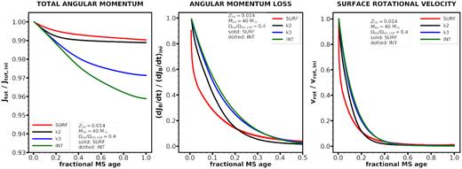
In this section, we present the results of the parameter tests. Fig. 1 illustrates the effects of wind magnetic braking on the evolution of the total angular momentum (left column), on the rate of angular momentum loss (middle column), and on the surface rotational velocity (right column), in all cases normalized to their initial values. The dependence on initial mass, rotational velocity, and magnetic field strength is shown as top, middle, and bottom panels, respectively. The ‘default’ model is the one with |$M_{\star , \rm ini} = 40$| M⊙, Ωini/Ωcrit,ini = 0.4, and Bp,ini = 5 kG at solar metallicity (Z = 0.014). The solid lines indicate models with surface magnetic braking (SURF), the dotted lines indicate models with internal magnetic braking (INT), and the dashed lines indicate non-magnetic models (NOMAG).
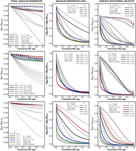
Evolution of the total angular momentum (left-hand panels), the angular momentum loss rate driven by the magnetic field and the gas (middle panels), and surface rotational velocity (right-hand panels) compared to their initial values. Varying the mass (top panels), rotation (middle panels), and magnetic field strengths (lower panels) is shown. Models with surface (internal) magnetic braking are shown with solid (dotted) lines. Non-magnetic models are shown with dashed lines. In all models the metallicity is Z = 0.014, and the same internal angular momentum transport processes are assumed for consistency.
4.1 Evolution of total angular momentum
4.1.1 Varying initial mass – panel (a)
In the case of non-magnetic models, the angular momentum loss due to stellar winds is stronger for higher mass models. For a non-magnetic 60 M⊙ model, the main-sequence angular momentum loss reaches about 1 per cent of its initial value. When surface magnetic braking is considered, the models lose the same relative amount of angular momentum, around 1 per cent, independent of their initial mass. When models account for internal magnetic braking, a larger amount of angular momentum is lost, which is the consequence of more efficiently distributing the losses and also more efficiently replenishing the surface angular angular momentum reservoir, keeping the surface angular velocity higher than in the SURF models. Thus the INT models, which mimic an efficient coupling by removing angular momentum from all layers of the star, always result in losing a larger amount of total angular momentum.
The 20, 40, and 60 M⊙ INT models lose the same amount of angular momentum at the end of the main-sequence phase (4 per cent),15 while the 10 M⊙ loses less (3 per cent), and the 5 M⊙ model loses about two times as much as the former ones (8 per cent).
Although the interesting behaviour of the 5 M⊙ model is amplified for the models with magnetic braking, this trend is also seen for the non-magnetic models. The reason why the lower mass model loses more angular momentum and brakes its surface rotation more rapidly is a consequence of various factors having counteracting effects.
Weaker winds (as is the case for lower initial mass) imply weaker angular momentum loss. On the other hand, the quantity of angular momentum that is lost at the surface depends also on the amount of angular momentum flowing from the inner regions of the star to the surface. The more rapid this transport, the larger the amount of angular momentum loss at the surface. The time-scale for this transport varies approximately as the radius of the star divided by the typical value for the meridional velocity in the stellar envelope. When the initial mass of the star decreases, both the radius and the meridional velocity decreases, so that it is difficult to predict what the result will be. Another factor is of course the duration of the main-sequence phase, the more extended it is, the larger the amount of angular momentum loss. The fact that the 5 M⊙ loses more angular momentum at the end of the MS phase than the 10 M⊙ is a consequence of all these factors combined.
4.1.2 Varying initial rotation – panel (b)
The non-magnetic and SURF models lose the same amount of angular momentum, while the INT ones lose larger amounts than those models. Nevertheless, in the former two cases, the evolution of the total angular momentum differs during the main sequence. The magnetic SURF models lose a larger amount of angular momentum than non-magnetic models at the beginning of the evolution. This is expected since during the early phases the star expands rather slowly and thus the surface magnetic field does not weaken fast. In the later phases, the SURF models lose less angular momentum because the surface magnetic field strength has decreased and the surface rotational velocity becomes low. The non-magnetic models, in contrast, lose more angular momentum at the end of the main-sequence phase, since at that stage they still have significant surface rotation and the mass-loss rates are higher.
4.1.3 Varying initial magnetic field strength – panel (c)
In this parameter test too, surface magnetic braking yields comparable total angular momentum loss as the non-magnetic model. This indicates that surface magnetic braking may only play a minor role in the total angular momentum evolution of the star. The SURF models initially lose more angular momentum, whereas the non-magnetic models lose more angular momentum at the end of their main-sequence phase. The angular momentum evolution of the INT models – in contrast to the other two types of models – shows a significant dependence on the initial surface magnetic field strength: the stronger the field, the larger the angular momentum loss.
4.2 Evolution of magnetic braking
4.2.1 Varying initial mass – panel (d)
The change of the rate of angular momentum loss is primarily attributed to the change in three parameters: (i) the increase of |$\dot{M}$|, (ii) the decline of Bp, and (iii) the decline of Ω⋆ over time. In a sense, this is a loop of consequences because as magnetic braking decreases the surface angular velocity, the strength of magnetic braking weakens as well (equation 1).
Above 10 M⊙, there is a clear dependence with stellar mass: magnetic braking weakens faster with higher stellar mass. In the case of the 5 M⊙ model, the fast decrease of magnetic braking is due to fast decrease in the surface rotation rates (panel g of Fig. 1).
4.2.2 Varying initial rotation – panel (e)
The differences between the INT and SURF models decrease when the initial rotation is higher. This is expected since in the SURF models increasing the surface rotation also increases the efficiency of the internal angular momentum transport by the meridional currents and thus these models are approaching the situation realized in the INT models. While the SURF models show a complex behaviour, the INT models reveal that for higher rotation rates the weakening of magnetic braking is more rapid.
4.2.3 Varying initial magnetic field strength – panel (f)
Varying the magnetic field strength shows that magnetic braking systematically weakens faster with stronger fields. Indeed, over a short time-scale strong fields lead to slowly rotating models, which will then have weak magnetic braking.
An essential component of the model calculations is to account for the time evolution of magnetic braking. This is in contrast with previous simplifying assumptions, which often extrapolated from current to zero-age main sequence (ZAMS) conditions, supposing a constant value of |$\frac{\mathrm{d}J_{B}}{\mathrm{d}t}$| over time (e.g. Petit et al. 2013). Such an assumption fundamentally breaks down and can be especially misleading when the current rotation is slow. We highlight the impact of this issue in Section 4.4.
Strong magnetic braking is not maintained during the entire main-sequence evolution (middle panels of Fig. 1) because the two necessary ingredients (strong magnetic fields and fast rotation) do not co-exist for considerable time-scales.
4.3 Evolution of surface rotation
4.3.1 Varying initial mass – panel (g)
The non-magnetic 5–20 M⊙ models only have a modest change in their surface rotation during the main sequence. If real stars followed such tracks, it would allow for approximating the value of the initial surface rotation just by measuring the actual one. Magnetic braking makes this connection no longer possible. Independent of the initial rotation or the braking method, all 40 M⊙ models with Ωini/Ωini,crit = 0.4 converge to an extremely slow surface rotation after one fifth of their main-sequence lifetime, that is about 1 Myr. Importantly, a low value measured presently does not preclude a high rotation in the past.
4.3.2 Varying initial rotation – panel (h)
All the 40 M⊙ models arrive at the Terminal Age Main Sequence (TAMS) with a similarly very low surface rotational velocity regardless the initial rotation.
In the non-magnetic case, the mass-loss by stellar winds is sufficient to remove a large amount of angular momentum. As already noted above for the most massive stars, this would not allow to trace back the initial rotation rates from measuring the surface rotation at an advanced stage of the main-sequence evolution. However, at a given fractional main-sequence age, the non-magnetic models have much higher surface rotational velocities than the magnetic models.
The SURF models are those presenting the most rapid drop off of the surface rotation. Again this is expected since in this case the time-scale for replenishing the outer layers with internal angular momentum is much longer than the magnetic braking time-scale. The rate of change of the rotation period is very different between the SURF and INT models and thus would represent a way to differentiate between these models, provided of course that some other constraints would allow to give information about the initial mass, metallicity, surface magnetic field, and fractional age.
4.3.3 Varying initial magnetic field strength – panel (i)
Clearly, the stronger the magnetic field, the more rapidly rotation brakes. At the early evolution, the INT models maintain a higher surface rotation with respect to the SURF models. In the INT models, the whole star is slowed down at the same time. In the SURF models (also in the non-magnetic one), initially only the outer layers are slowed down hence the more rapid decrease of the surface rotation.
4.4 Impact on spin-down age determination
The spin-down age derived by Petit et al. (2013) relies on two important assumptions:
The rate of angular momentum loss is constant with time.
At any time, the surface rotation is directly tied to the total angular momentum of the star, such that solid-body rotation is achieved.
We have shown that the first assumption is not justified because magnetic braking evolves with time (Section 4.2), and it remains unknown whether stars could be characterized as solid-body rotators or not.
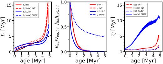
Estimated spin-down age (left-hand panel), normalized rotational velocity and total angular momentum (middle panel), and spin-down time-scale (right-hand panel) versus the age of the modelled star. The two default 40 M⊙ SURF and INT models are shown as described in Section 4.
The evolution of the surface rotational velocity (solid lines, middle panel) is closely tied to the evolution of the total angular momentum (dashed lines) in the INT case, whereas for the SURF case, the evolution of the surface rotational velocity and the total angular momentum are decoupled (making the second assumption inappropriate). For the INT model, both the estimated spin-down time-scale and the model spin-down time-scale (|$J/\frac{\mathrm{d}J}{\mathrm{d}t}$|) are approximately constant over the first few Myr (right-hand panel). This means that the spin-down age only begins to significantly deviate from the real age once the star is close to the TAMS – in this particular set-up.
5 PROGENITORS OF SLOW ROTATORS
Fig. 3 shows models of massive stars with initially 15 M⊙. The inclusion of surface fossil magnetic fields results in two notable features on the HRD: (i) models with the same initial mass and initial field strength but different initial rotational velocities follow the same track after their early evolution, leading to a degeneracy between them, and (ii) the evolutionary track of an initially fast-rotating magnetic model differs significantly from an initially fast-rotating non-magnetic model.
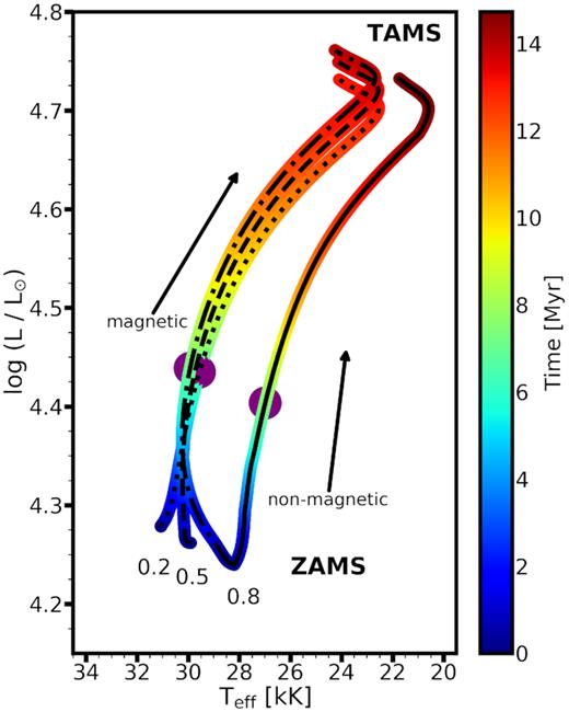
Models with different initial ratios of Ω/Ωcrit (indicated next to the tracks: 0.2 dotted line, 0.5 dashed line, 0.8 dash–dotted line, respectively) are shown in the case of the 15 M⊙ models with an initial polar field strength of 3 kG. A reference non-magnetic model (solid line) is also shown with the same mass and an initial ratio of Ω/Ωcrit = 0.8. The colour coding indicates the time after ZAMS and the purple markers show the location at which the model is exactly half-way through its main-sequence lifetime. Models with surface magnetic braking are shown.
With higher rotational velocities, the ZAMS position of the tracks is shifted to lower luminosity and effective temperature. This is due to the mechanical effects of rotation: the centrifugal force contributes to balance gravity. The rapidly rotating model therefore has a ZAMS position that resembles of a non-rotating star with a lower initial mass. Since the wind magnetic braking slows down the surface rotation of the star, the magnetic models converge towards the slow-rotating case independent of the initial rotation.
However, when magnetic braking is absent, the star retains more angular momentum and the track remains in the redder part of the HRD due to the mechanical effects of rotation, that is, the star evolves with lower effective temperature. If the mixing was more efficient, it would result in a blueward evolution on the HRD. For fast-rotating models, a blueward evolution is indeed associated with chemically homogeneous evolution (see e.g. fig. 6 of Brott et al. 2011a). Contrary to that, the quantitative differences in the initially rapidly rotating magnetic model arise from the fast disappearance of the initial centrifugal support, which leads to the tracks converging towards the slow-rotating case.
Finally, if observed stars were attempted to be reconciled with non-magnetic evolutionary models, their physical parameters would only be consistent with initially slowly rotating models. Instead, observed stars should also be contrasted with models that initiate their evolution as rapid rotators but brake their rotation due to magnetic braking. The physical characteristics of the two models (initially slow and fast rotators, respectively) are different.
For reference, at half-way through their main-sequence evolution (shown with purple markers on Fig. 3) the magnetic (SURF) and non-magnetic models with Ωini/Ωini,crit = 0.8 have stellar ages of 6.9 and 7.3 Myr, while at the TAMS their ages are 13.9 and 14.7 Myr, respectively (see Tables C1 and C2). This may lead to systematic shifts in the estimated stellar ages of observed stars, therefore it has to be considered when comparing observed magnetic massive stars with evolutionary models that do not account for surface magnetic fields (Fossati et al. 2016; Schneider et al. 2016; Shultz et al. 2018).
6 COMPARISON OF MODEL PREDICTIONS WITH THE POPULATION OF MAGNETIC B-TYPE STARS
Shultz et al. (2018) presented high-resolution magnetometry and obtained rotation periods for the known population (55) of main-sequence magnetic B-type stars with spectral types between B5 and B0. We use this sample of magnetic stars to evaluate our magnetic B-star evolutionary models. Atmospheric parameters for these stars based upon spectroscopic modelling and Gaia data release 2 parallaxes were presented by Shultz et al. (2019a). Shultz et al. (2019c) combined these observables to calculate fundamental stellar parameters, magnetic parameters (assuming an inclined dipole topology), stellar wind parameters, and magnetospheric parameters. The estimated masses of the observed stars range from 4.3 to 17.5 M⊙, and were determined from the non-magnetic evolutionary models of Ekström et al. (2012).
To facilitate a more straightforward comparison, we separated the observed stars into three mass bins: |$M_\star \lt 7.5\, \mathrm{M}_\odot$|, 7.5 < M⊙ < 12.5, and |$\mathrm{M}_\odot \gt 12.5\, \mathrm{M}_\odot$| (coloured with green, blue, and red in Figs 4–6), and we computed 5, 10, and 15 M⊙ models correspondingly. Known short-period (Porb < 2 d) binary stars (HD 37017, HD 149277, HD 136504, HD 156324, HD 36485) are shown with open symbols.
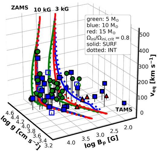
Shown are the surface equatorial rotational velocities, the dipolar magnetic field strength, and the logarithmic surface gravities of the observed stars and model predictions. The observations are separated into three mass bins: 5 (green circles), 10 (blue squares), and 15 (red triangles) M⊙. Models with Ωini/Ωini,crit = 0.8 and Bp,ini = 3 and 10 kG are shown. Known short-period binaries are shown with open symbols.
6.1 Evolution of surface rotation and magnetic field strength
Fig. 4 shows the evolution of surface rotational velocity and magnetic field strength, in terms of the surface gravity. The 3D plot shows models with initially 3 and 10 kG fields, initiating their evolution on the top left and evolving towards the lower right of the diagram. This diagram emphasizes that the models need to account for multiple observables simultaneously. The left-hand panel of Fig. 5 further details the rotational evolution, and models with different initial rotation rates are shown for the 3 kG field strength, which was chosen as Shultz et al. (2019c) found a mean field strength close to that value. The right-hand panel of Fig. 5 displays the magnetic field evolution, showing models with varying magnetic field strength, keeping the initial ratio of Ω/Ωcrit = 0.8. On all three diagrams, the colour coding represents stellar mass (see caption).
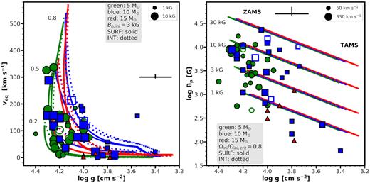
Shown are the surface equatorial rotational velocities (left-hand panel) and dipolar magnetic field strengths (right-hand panel) versus the logarithmic surface gravities. The colours follow the description of Fig. 4. The mean errorbars are indicated to the centre right and top, respectively. Markers vary in size corresponding to the measured dipolar field strength of observed stars (left-hand panel) or the surface equatorial rotational velocities (right-hand panel). Left-hand panel: Models with Ωini/Ωini,crit = 0.2, 0.5, 0.8 and an initial polar magnetic field strength of 3 kG are shown. Right-hand panel: Models with Ωini/Ωini,crit = 0.8 and an initial polar magnetic field strength of 1, 3, 10, and 30 kG are shown.
6.1.1 Rotational evolution of known magnetic B-type stars
From Figs 4 and 5 it can be immediately seen that there is a generally good agreement between models and observations: as expected, the rotation rapidly decreases with decreasing surface gravity. However, for currently slow-rotating stars, magnetic braking inhibits our ability to access their prior rotational history, and in particular how rapidly they might have been rotating initially. We emphasize again that this result is only achieved when surface magnetic fields are accounted for in the models; otherwise, in general, only initially slow-rotating (or, in practice, non-rotating) models are consistent with observations of currently slow-rotating stars.
The median equatorial surface rotational velocity of the sample stars is 78 km s−1 and more than half of the sample stars have a surface rotational velocity less than 100 km s−1. It is also apparent that the most massive stars in the sample are all slow rotators (<50 km s−1). A smaller fraction of stars (36.3 per cent) is located between 100 and 200 km s−1, while three single stars and one binary star (7.3 per cent) have notably high rotational velocities (>200 km s−1).
While, in general, the agreement between the models and observations is good, a striking discrepancy (in particular, on the left-hand panel of Fig. 5) is seen in the case of HD 122451Ab (log g = 3.55, veq = 154 km s−1, Bp ≈ 230 G), which is in a triple system and a known β Cep pulsator (Pigulski et al. 2016). The orbital period of the two closer components (HD 122451Aa,b) is nearly 1 yr, on a highly eccentric orbit. It can therefore be speculated that the magnetic star gains angular momentum from the orbital reservoir, and thus rotates more rapidly than expected from a single star undergoing magnetic braking.
The three most rapidly rotating (>200 km s−1) single stars in the sample (HD 182180, HD 142184, HD 345439) require some more attention. These stars have order of 10 kG dipolar magnetic fields, consistent with the mean strength near the ZAMS, where their high log g values indicate they reside. Their rapid rotation is further consistent with a young age. Importantly, our models predict no such stars should be present except at very young ages, as is indeed the case.
The presence of young and rapidly rotating magnetic stars is interesting in light of theoretical considerations regarding the ZAMS rotation rates of magnetic stars. The fossil field hypothesis relies on the long-term stability of magnetic fields and assumes that these fields were generated during the star formation process or at the latest during the pre-main-sequence evolution of the star (Donati & Landstreet 2009). In lower mass Ap and Herbig Ae/Be stars, pre-main-sequence magnetic braking is indeed evidenced (Stȩpień 2000; Alecian et al. 2013). This could also be the case for O and B stars (where the pre-main-sequence phase and the magnetic fields are not practically observable due to these stars being embedded in dust). However, the contraction time-scale is shorter than the magnetic braking time-scale, hence a magnetic star can arrive at the ZAMS as a fast rotator. In fact, initially moderate and high rotation rates at the ZAMS are clearly required to explain almost half of the sample of known magnetic B stars. Therefore, reconciling the rapidly rotating stars with our models leads us to conclude that they must initiate their main-sequence evolution with nearly critical rotation. If, on the other hand, these stars did not start their main-sequence evolution as rapid rotators, consideration of spin-up mechanisms would be required.
An intriguing scenario is to explain the observed rapid rotation of some stars via the binary channel, assuming that a companion star may be responsible for either halting magnetic braking or, in fact, spinning up the magnetic star via tidal interactions or mass transfer. Indeed, a significant fraction of OB stars are expected to be in binary systems (de Mink et al. 2014; Sana et al. 2014). As of now there is no observational evidence that either of the three rapidly rotating stars has a close companion star. However, if such a surprising discovery was made, it would provide a natural explanation for their short rotation periods. Since the incidence rate of magnetism in close binary system is very low (Alecian et al. 2013), another alternative to the binary channel is that magnetic massive stars may be merger products, thus initially a system of two (pre-) main-sequence binary stars (Ferrario et al. 2009; Schneider et al. 2016). This may also result in a rapidly rotating star, although likely only for a short time-scale. Interestingly, in recent numerical simulations of binary mergers, Schneider et al. (2019) obtain a post-merger object with a moderate rotational velocity (≈200 km s−1) at the ZAMS.
6.1.2 Magnetic evolution of known magnetic B-type stars
Figs 4 and 5 show that, in general, models with a large range of initial magnetic field strength are in agreement with observations.
Shultz et al. (2019c) showed that no clear trend could be identified between Bp and M⋆ (their fig. 9), and they argued that the magnetic field strength may decrease more rapidly than expected from magnetic flux conservation (see also Landstreet et al. 2007, 2008; Fossati et al. 2016). Indeed, the weaker magnetic fields of the more massive B-type stars are a consequence of those stars being more evolved.
A few presumably evolved stars with weak magnetic fields are not matched by the computed models (see Figs 4 and 5). Since the observed magnetic field strengths span a large range, it may be possible that those stars with low values of log g and Bp simply initiated their evolution with weaker fields than considered in our models (<1 kG). However, their progenitors (with high log g and low Bp) remain undetected. Another piece in this puzzle is the lack of descendants with strong fields (which are easier to detect) but lower surface gravity. The absence of such stars is consistent with previous suggestions that the magnetic fields of OB stars are subject to a flux decay mechanism, in contrast to the evolution of the magnetic fields of A and Ap stars which are consistent with flux conservation (Landstreet et al. 2007; Neiner et al. 2017; Sikora et al. 2019). The flux decay rate could, in principle, be inferred empirically by matching the observed relationship of log g and Bp. If a field decay in the computed models needed to be accounted for, then the tracks with given initial field strength would show lower magnetic field for a given surface gravity. On the other hand, this weakening may affect the rotational evolution, which will need to be studied in detail with models accounting for different field evolution scenarios.
6.2 Evolution of rotation and confinement
The rotation-confinement diagram (Fig. 6, see also fig. 3 of Petit et al. 2013, fig. 7 of Paper I, and fig. 8 of Shultz et al. 2019c) shows the relative importance of magnetic wind confinement and centrifugal support in terms of the Alfv´en radius and the Keplerian co-rotation radius (equations 3 and 4). The overwhelming majority of the observed B-type stars are in the CM regime (see Section 2). The significance of the magnetospheric characterization is related to the age determination of observed stars, as stars with CMs are typically expected to be young, whereas stars with dynamical magnetospheres (DMs) are expected to be evolved (Petit et al. 2013, Paper I, Shultz et al. 2019c).
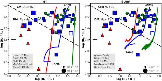
Shown is the rotation-confinement diagram, i.e. the Alfv´en radius versus the Kepler co-rotation radius. The observations are separated into three mass bins: 5 (green circles), 10 (blue squares), and 15 (red triangles) M⊙. Models with Ωini/Ωini,crit = 0.8 and an initial polar field strength of 10 kG are shown. Known short-period binaries are shown with open symbols. The marker size corresponds to the logarithmic surface gravity. The mean errorbars are shown to the centre left. DM and CM indicate dynamical and centrifugal magnetospheres, respectively. The model evolution begins at the top right corner of the diagrams. Left: internal magnetic braking. Right: surface magnetic braking.
The evolutionary models shown in Fig. 6 have an initial field strength of 10 kG. Shultz et al. (2019c) found that all early B-stars in the final third of their main sequence lifetimes have DMs. The absence of evolved stars with CMs is consistent with the typical ZAMS surface magnetic field strength being higher than 1 kG.
The stars in the 15 M⊙ mass bin from the Shultz et al. (2018) sample have a DM, therefore they are expected to be evolved. However, they are not matched with the computed models on the RK–RA plane. A possible explanation is that the magnetic field strength weakens more rapidly than expected from magnetic flux conservation (see previous section), in which case the decrease in RA is more rapid, thus our tracks on the diagram would indicate lower RA values for given RK. This correction could reconcile the discrepancy. Another possibility is if magnetic braking was much more efficient on the pre-main sequence for more massive stars, so they arrive at the ZAMS already as slow rotators. It could also be that at least some magnetic stars follow an unusual trend on the HRD. In particular, HD 149438 (τ Sco) may be a blue straggler and is a promising candidate for a merger product (Schneider et al. 2016, 2019). Furthermore, τ Sco is also a significant example of a magnetic star that may present an apparently younger age than the age of the cluster that it belongs to (Nieva & Przybilla 2014; Schneider et al. 2016). If this is a general trend, this would mean that for the sample stars the cluster ages may overestimate their actual age.
The stars in the 10 M⊙ bin show a scatter, however, leading to similar findings as in the case of the 15 M⊙ stars. The stars in the 5 M⊙ bin are all located in the CM regime (except one star). This is consistent with their rotational and magnetic field evolution as both surface rotation and magnetic field strength show high values (Figs 4 and 6). This suggests that these stars are mostly in their early evolutionary stage, in agreement with the findings of Shultz et al. (2019c). The INT models predict 5–10 M⊙ stars in the lower part of the diagram (large RA, small RK, see Fig. 6), while the SURF models do not. The latter case seems more consistent with the lack of such observations.
All known close binary stars are in the CM regime. Indeed, HD 36485, HD 37017, and HD 156324 are in the extreme CM regime and display H α emission, which correlates strongly with strong magnetic confinement, rapid rotation, and young stellar age. However, to what degree this is a consequence of tidal acceleration is not clear. The three binary stars showing H α-emission are all very young, and their CMs are no larger than single H α-bright stars of comparable ages (Shultz et al. 2019c). The two close binary systems without H α emission, HD 136504 (in which system both components are magnetic, Shultz et al. 2015) and HD 149277, are middle-aged and have CMs that are somewhat smaller than the average of their contemporaries.
6.3 Remarks from the model validation from the comparison with known magnetic B-type stars
The purpose of this initial comparison between state-of-the-art models and a sample of observed magnetic B-type stars was to validate the models that contain a prescription of surface fossil magnetic fields. We found that in general the models are in good agreement with the observations when considering their rotational and magnetic evolution alone.
Three observed (presumably single) stars and some stars with moderate rotation (100–200 km s−1) are only compatible with initially (at least) moderately or rapidly rotating models. The rest of the sample (consisting of mostly older, slowly rotating stars) leads to a degenerate solution to determine their initial rotation rates. Observations require models with a range of initial rotational velocities. This has an impact on star formation theory, which will have to account for both the fast and slow ZAMS rotation of massive stars with surface fossil magnetic fields.
There is no striking discrepancy between the models and observations when looking at the magnetic field evolution alone. However, from the rotational and magnetospheric diagnostics, one could argue that a systematic discrepancy is introduced by adopting magnetic flux conservation as the modelled field evolution. Indeed, a systematic shift of the models is expected if magnetic flux decay (i.e. a more rapid decline than expected from the |$\propto R_\star ^{-2}$| dependence alone) can be quantified and hence implemented in our models. This could potentially be the key to reconciling the evolution seen on the RK–RA plane.
7 CONCLUSIONS
In this work, we described the implementation of magnetic braking applicable for hot, massive stars in the mesa software instrument, and studied the rotational evolution of the models. We provide the scientific community with this additional mesa module that contains a realistic and simple prescription of surface fossil magnetic fields in stellar evolution codes (see also Georgy et al. 2017; Keszthelyi et al. 2017a; Petit et al. 2017; Paper I). We emphasize, however, that this implementation needs to be improved to consider additional components for a more comprehensive picture.
Presently, there exists no verified formalism that could treat internal angular momentum transport by a fossil field in massive stars; although some approaches have been explored – and many more in the context of dynamo-generated fields. In principle, the contribution from Poynting stresses could be considered in a similar manner; however, the picture is likely to be far more complex and first the interaction with hydrodynamical instabilities would need to be established. Empirical evidence may be collected soon with the advent of magneto-asteroseismology (Buysschaert et al. 2018; Prat et al. 2019), and it will be invaluable to guide evolutionary modelling. One of the key uncertainties remains the internal effects of the fossil field and the extent to which they are anchored inside the star. We hope that the parametrization developed in this work will become a convenient tool to adjust the number of torqued layers in the stellar model. To improve on the implementation presented in this work, one may consider coupling it with other approaches that focused on different aspects. For example, the interaction of fossil fields and convection (Featherstone et al. 2009; Petermann et al. 2015; MacDonald & Petit 2019), structural changes by the fossil field (Mathis & Zahn 2005; Duez & Mathis 2010; Prat et al. 2019), the magnetorotational instability (Wheeler, Kagan & Chatzopoulos 2015; Quentin & Tout 2018), and appropriate angular momentum transport (Spruit 2002; Heger et al. 2005; Maeder & Meynet 2005; Denissenkov & Pinsonneault 2007; Rüdiger et al. 2015; Kissin & Thompson 2018; Fuller et al. 2019; Schneider et al. 2019) would be required to establish altogether a more coherent picture regarding the effects of surface fossil magnetic fields.
The models presented in this study are one-dimensional. As such, they naturally ignore any variations in co-latitude. Based on current two-dimensional MHD simulations, it is not clear how well the assumed angular momentum loss via magnetic braking (equation 1) applies in more realistic three-dimensional situations where the magnetic field is tilted with respect to the rotation axis. It is possible that the tilt would only lead to minor corrections in the formalism and our assumptions here are still appropriate.
We found that the time evolution of magnetic braking is an essential component since it is rapidly weakened by stellar feedback effects – primarily via decreasing the surface rotational velocity. We demonstrated that internal magnetic braking can greatly deplete the total angular momentum reservoir, whereas surface magnetic braking allows the star to maintain most of its total angular momentum.
With the inclusion of surface fossil magnetic fields in stellar evolution models, we identified that initially fast-rotating magnetic models undergo an early blueward evolution. Models with given surface fossil magnetic fields and initial mass but different initial rotation rates, merge to a common track, leading to a degeneracy to disentangle between their initial rotation rates. Therefore, further considerations are required before gyrochronology could be applied to magnetic massive stars. Moreover, we showed that initially fast-rotating magnetic stellar models evolve quite differently than non-magnetic ones, causing a significant discrepancy in the derived stellar ages, amongst others.
Comparing our models with observations from Shultz et al. (2018), we found that most likely a range of initial rotation rates is required to explain both slowly and rapidly rotating young magnetic B-type stars. This has potential consequences to explain the formation of magnetic massive stars. Furthermore, this may help to shed more light on fossil field evolution: if magnetic massive stars arrive at the ZAMS with close to critical rotation, then pre-main-sequence magnetic braking is either inefficient or absent.
Models with surface and internal magnetic braking were shown to be non-interchangeable: they produce different results. Both our SURF and INT models might be compatible with the comprehensive sample of known magnetic B-type stars of Shultz et al. (2018). Further studies should be conducted to evaluate these scenarios.
ACKNOWLEDGEMENTS
We thank the anonymous referee for providing us with a constructive and helpful report, which has led to improving the paper. We appreciate discussions with K. Augustson and P. Marchant. We are grateful for B. Paxton and the mesa developers for making their code publicly available. GM and CG acknowledge support from the Swiss National Science Foundation (project number 200020-172505). MES acknowledges support from the Annie Jump Cannon Fellowship, which supported by the University of Delaware and is endowed by the Mount Cuba Astronomical Observatory. AuD acknowledges support from NASA through Chandra Award number TM7-18001X issued by the Chandra X-ray Observatory Center, which is operated by the Smithsonian Astrophysical Observatory for and on behalf of NASA under contract NAS8-03060. RHDT acknowledges support from National Science Foundation grants ACI-1663696 and AST-1716436. GAW acknowledges support in the form of a Discovery Grant from the Natural Science and Engineering Research Council (NSERC) of Canada. VP acknowledges support provided by (i) the National Aeronautics and Space Administration through Chandra Award Number GO3-14017A issued by the Chandra X-ray Observatory Center, which is operated by the Smithsonian Astrophysical Observatory for and on behalf of the National Aeronautics Space Administration under contract NAS8-03060, and (ii) program HST-GO-13734.011-A that was provided by NASA through a grant from the Space Telescope Science Institute, which is operated by the Association of Universities for Research in Astronomy, Inc., under NASA contract NAS 5-26555. ADU acknowledges support from NSERC.
Footnotes
Hot stars do have thin subsurface layers where inefficient convection (accounting for usually ≈3 per cent of the energy transport) occurs due to the iron opacity bump (Cantiello et al. 2009), and while there might perhaps be dynamo activity in those layers (Cantiello & Braithwaite 2011), that would not give rise to the strong, globally organized fields which are observed in magnetic OB stars.
see Appendix A for more details.
see the summer school material by M. Cantiello: https://doi.org/10.5281/zenodo.2603726.
These quantities are in units of the cgs system.
We will use a notation that is consistent with the mesa instrument papers (Paxton et al. 2013).
In the previous equations, we did not introduce negative signs and the mass-loss rate in equation (1) appears with a positive sign.
We note that while solid-body rotation is not enforced per se, in practice the rotation profile of the INT models is nearly flat during the magnetic braking time-scale. This is because angular momentum transport via meridional currents remains efficient in the model.
We only consider single stars, but evidently the situation is different in binary or multiple systems.
This means that when implementing the prescription of magnetic braking (equation 1), the mass-loss driven angular momentum loss needs to be subtracted to avoid double counting.
We caution that these results are based on a sample of low- and intermediate-mass stars below 8 M⊙, therefore the conclusions may differ for massive stars. Measurements of the rotation profiles of massive stars are still largely lacking.
The mass-loss quenching parameter fB was shown to contain a small correction term when models with rotation are considered (ud-Doula et al. 2009). To the first order, we neglect this in this study since, for example, the appropriate geometrical correction for oblique rotation and the latitudinal mass-flux dependence may lead to a much more notable impact. Nevertheless, we recommend taking it into account in future approaches.
We systematically use Ω to denote the angular velocity (and Ω⋆ to denote the surface angular velocity), although some other conventions prefer ω. Since in the computed models the equatorial and polar radii differ negligibly, we follow the mesa definition to adopt the critical value of the angular velocity as |$\Omega _{\rm crit} = \sqrt{(1-\Gamma) \frac{GM_\star }{R_\star ^3} }$|. This is none the less only used as an input for setting the initial rotation rates, but not for our calculations.
The 40 and 60 M⊙ INT models, represented with green and grey dotted lines, practically overlap on the diagram.
Presently it remains unclear how the spin-down time-scale of the model with surface magnetic braking could be appropriately described. In that case, it is only the surface angular momentum reservoir which is being exhausted not the total angular momentum of the star. However, it is further complicated by the presently unknown angular momentum transport inside the star, which could replenish the surface reservoir with angular momentum from the stellar core.
REFERENCES
APPENDIX A: IMPLEMENTATION IN genec
The structure of the star in genec is slightly different to the mesa one. The main differences are the following:
In genec, the structure equations, chemical composition evolution equations, and rotation equations are decoupled and solved one after the other iteratively up to a converged structure is reached at a given time-step. In mesa, the whole set of coupled equations is solved at once.
In genec, the star is divided into three different regions (see also Kippenhahn & Weigert 1990): the interior, going from the centre of the star to a given ‘fitting point’, located at a mass coordinate Mfit inside the star; the envelope, going from Mfit to the point where an optical depth of τ = 2/3 is reached; the atmosphere, providing the boundary conditions. In the interior, the whole set of equations is solved. In the envelope, the energy generation rate is assumed to be zero, the chemical composition constant, and the rotation uniform (see Maeder 2009, for more details).
- The time evolution of the angular momentum transport in genec is computed by solving the following advecto-diffusive equation (Maeder & Zahn 1998):with r the radius, ρ the density, Ω the angular velocity, U(r) the radial component of the meridional circulation, and D a diffusion coefficient accounting for various instabilities. This equation is solved following an operator-splitting approach, where the advective part and the diffusive part are solved alternatively every two time-steps. mesa uses a fully diffusive approximation, which is practically identical to equation (A1) without the advective term (the first term on the r.h.s.).(A1)$$\begin{eqnarray} \rho \frac{\text{d}}{\text{d}t}(r^2\Omega)_{M_r} = \frac{1}{5r^2}\frac{\partial }{\partial r}(\rho r^4\Omega U(r)) + \frac{1}{r^2}\frac{\partial }{\partial }\left(\rho Dr^4\frac{\partial \Omega }{\partial r}\right), \end{eqnarray}$$
To account for magnetic braking in genec, an additional torque is applied as a boundary condition to equation (A1) (see Eggenberger et al. 2008, for a detailed discussion). In this framework, the fitting mass Mfit plays the same role as the mass Mt described in the discussion about the implementation in mesa. However, instead of assuming that the same fraction of the angular momentum is lost in each layer, this zone is assumed to rotate as a solid body, and the angular momentum is removed in the entire region keeping solid-body rotation.
APPENDIX B: CONVERGENCE TEST BETWEEN THE SURF AND INT CASES
In the following parameter test, the same input is used as described for our ‘default’ (M⋆,ini =40 M⊙, Ωini/Ωini,crit = 0.4, Bp,ini = 5 kG) model. For the four models presented in Fig. B1, the number of torqued layers vary as follows: SURF denotes the case when |$x = k\_const\_mass$| as described in Section 3.2, k2 denotes |$x = 2 \cdot k\_const\_mass$|, k3 denotes |$x = 3 \cdot k\_const\_mass$|, and in the INT case the angular momentum loss is distributed to every layer of the star. Since the number of layers is increased, in practice, this corresponds to distributing the angular momentum loss to larger and larger mass fractions of the star. Thus, we verify that the SURF case tends toward the INT case when the number of torqued layers is increased.
Evolution of the total angular momentum, the angular momentum loss rate driven by the magnetic field and the gas, and surface rotational velocity compared to their initial values. k2 and k3 denote models where the number of torqued layers is doubled and tripled compared to the SURF case.
APPENDIX C: TABLES
15 M⊙ model comparison at half-way through their main-sequence lifetimes from Fig. 3 (indicated with purple marker).
| Model | Braking scheme | |$\frac{\Omega _{\rm ini}}{\Omega _{\rm crit, ini}}$| | Teff | log L/L⊙ | M⋆ | log g | vrot | log Jtot | Age |
|---|---|---|---|---|---|---|---|---|---|
| (kK) | (M⊙) | (cm s−2) | (km s−1) | (g cm2 s−1) | (Myr) | ||||
| MAG | INT | 0.2 | 29.541 | 4.435 | 14.994 | 4.014 | 38.946 | 51.528 | 6.532 |
| MAG | INT | 0.5 | 29.508 | 4.433 | 14.994 | 4.014 | 82.860 | 51.838 | 6.583 |
| MAG | INT | 0.8 | 29.605 | 4.433 | 14.994 | 4.020 | 90.946 | 51.874 | 6.683 |
| MAG | SURF | 0.2 | 29.561 | 4.435 | 14.994 | 4.015 | 20.364 | 51.825 | 6.551 |
| MAG | SURF | 0.5 | 29.715 | 4.438 | 14.994 | 4.021 | 49.061 | 52.012 | 6.769 |
| MAG | SURF | 0.8 | 29.923 | 4.439 | 14.994 | 4.032 | 51.828 | 52.048 | 6.944 |
| NOMAG | – | 0.8 | 26.983 | 4.404 | 14.888 | 3.885 | 514.516 | 52.540 | 7.363 |
15 M⊙ model comparison at the TAMS from Fig. 3.
| Model | Braking scheme | |$\frac{\Omega _{\rm ini}}{\Omega _{\rm crit, ini}}$| | Teff | log L/L⊙ | M⋆ | log g | vrot | log Jtot | Age |
|---|---|---|---|---|---|---|---|---|---|
| (kK) | (M⊙) | (cm s−2) | (km s−1) | (g cm2 s−1) | (Myr) | ||||
| MAG | INT | 0.2 | 24.007 | 4.731 | 14.982 | 3.357 | 6.134 | 50.904 | 13.059 |
| MAG | INT | 0.5 | 24.040 | 4.731 | 14.982 | 3.360 | 10.488 | 51.080 | 13.163 |
| MAG | INT | 0.8 | 24.122 | 4.736 | 14.983 | 3.361 | 7.433 | 50.945 | 13.362 |
| MAG | SURF | 0.2 | 24.089 | 4.731 | 14.982 | 3.363 | 8.737 | 51.683 | 13.100 |
| MAG | SURF | 0.5 | 24.124 | 4.749 | 14.981 | 3.348 | 10.381 | 51.816 | 13.538 |
| MAG | SURF | 0.8 | 24.258 | 4.761 | 14.980 | 3.345 | 8.565 | 51.832 | 13.887 |
| NOMAG | – | 0.8 | 21.732 | 4.732 | 14.542 | 3.170 | 306.788 | 52.305 | 14.726 |
