


ABSTRACT
We consider the size distribution of superbubbles in a star-forming galaxy. Previous studies have tried to explain the distribution by using adiabatic self-similar evolution of wind-driven bubbles, assuming that bubbles stall when pressure equilibrium is reached. We show, with the help of hydrodynamical numerical simulations, that this assumption is not valid. We also include radiative cooling of shells. In order to take into account non-thermal pressure in the ambient medium, we assume an equivalent higher temperature than implied by thermal pressure alone. Assuming that bubbles stall when the outer shock speed becomes comparable to the ambient sound speed (which includes non-thermal components), we recover the size distribution with a slope of ∼−2.7 for typical values of interstellar medium pressure in Milky Way, which is consistent with observations. Our simulations also allow us to follow the evolution of size distribution in the case of different values of non-thermal pressure, and we show that the size distribution steepens with lower pressure, to slopes intermediate between only-growing and only-stalled cases.
1 INTRODUCTION
The distribution of sizes of superbubbles created by stellar winds and supernovae (SNe) of OB associations can be a diagnostic of the star formation process in a galaxy. The seminal paper by Oey & Clarke (1997) [hereafter OC97] showed that if the mechanical luminosity function of OB associations is described by a power law , ϕ(L) ∝ L−β, then for a constant star formation rate (SFR), the differential size distribution of superbubbles is given by N(R) ∝ R1 − 2β, for bubbles whose evolution is dominated by ambient pressure and have stalled. For typical parameters, OC97 estimated this stalling radius to be ≤1 kpc, which implies that observed superbubbles are in this phase of evolution. This robust prediction of the size distribution to have a power law with index 1 − 2β makes it a useful diagnostic of the star formation process in a galaxy. This predicted distribution has been confirmed by The HI Nearby Galaxy Survey, which studied the properties of H i holes in nearby galaxies (Bagetakos et al. 2011). They found that the size distribution has a power-law index of ∼−2.9, which implies β ≈ 2, which in turn is consistent with independent observations of OB association (McKee & Williams 1997).
The robustness of this predicted size distribution, however, raises the question whether or not it depends on parameters such as ambient pressure, density, and so on, and if so, how. Since it was derived assuming that ambient pressure does not affect the adiabatic expansion of a stellar wind bubble (Weaver et al. 1977) other than to impose a stall criterion, it is not possible to answer these questions without going beyond these assumptions. Although the average distribution in THINGS came out to have a power law of ∼−2.9, individual galaxies had distributions whose power law ranged between −2 and −4. Early-type spiral galaxies showed a steeper slope than late-type spirals and dwarf galaxies. Bagetakos et al. (2011) explained this by invoking the fact that scale heights of discs in early-type spirals are smaller than in late-type spirals, and are easy to break out of. This would limit the size of the largest holes, and consequently steepen the size distribution. However, one could also envisage a scenario in which a truncated or steepened OB association luminosity function in early-type galaxies produce a steep size distribution of H i holes, as is known to also manifest in the H ii region luminosity function (Oey & Clarke 1998). In order to disentangle the effects, one would have to calculate the size distribution beyond the assumptions of adiabaticity, which is inherent in the self-similar evolution of bubbles. And then the question remains as to how the power-law distribution with index ∼−3 derived from such assumptions match the observations.
In this paper, we relax the assumptions of self-similarity in the bubble evolution, include radiative cooling, with the help of 1D hydrodynamic numerical simulation, and derive the size distribution. We assume a constant SFR for simplicity. The paper is structured as follows. We first review the results of OC97 in light of Monte Carlo simulations in Section 2. Then, we discuss the results when ambient pressure is included in the dynamics of superbubbles, in Section 3. In Section 4, we discuss the effects of cooling and present the results in Section 5. The implications are discussed in Section 6.
2 SELF-SIMILAR SUPERBUBBLES
We first review the essence of OC97 calculations. They assumed that the mechanical luminosity function of OB association is given by ϕ(L) ∝ L−β. The luminosity of each cluster is assumed to be constant in time, until the lowest mass SN progenitors expire at te ∼ 40 Myr. The wind bubble is assumed to evolve in a self-similar manner, so that the radius scales as, R ∝ L1/5t3/5 (Weaver et al. 1977). Note that this assumes adiabatic expansion of the bubble. The pressure inside then evolves as pi ∝ L2/5t−4/5. If the ambient pressure is p0, then these bubbles are assumed to stall when p0 = pi. This implies a stalling time, for the bubble to reach a final radius, of tf ∝ L1/2. This in turn leads to a scaling of the final stalling radius |$R_\mathrm{ f} \propto L^{1/5} t_\mathrm{ f}^{3/5} \propto L^{1/2}$|.
The size distribution of bubbles is shown in Fig. 1, for different times after the onset of star formation, for bubbles growing in a self-similar manner as mentioned above. The ambient pressure is assumed to be P0 = 2.76 × 10⁻¹² dyne cm−2 as was considered by OC97. As expected from the arguments in OC97, the dominant slope of the distribution is roughly 1 − 2β = −3, for radii below the maximum size of stalled bubbles at a given epoch. OC97 estimated the stalling time-scale and the stalled sizes. Initially, low-luminosity bubbles stall, and at a given epoch, bubbles up to a certain size stall, beyond which the bubbles are in a growing phase. We show this upper limit of stalled sizes with square boxes on the red and blue lines, corresponding to 5 and 10 Myr (using equation 31 of OC97). (At later times, the biggest stalled bubbles cross the limit of sizes considered by us.) Fig. 1 shows that the fitted power laws until this maximum size has an index close to −3. However, there is also another class of small bubbles that are growing at any given epoch, arising from either massive but young clusters or low-mass clusters.

Size distribution of self-similar superbubbles for a constant SFR at different epochs, for an ambient pressure p0 = 2.76 × 10⁻¹² dyne cm−2, and ambient temperature Tamb = 4 × 10⁴ K. The square boxes on the blue and red lines show the values of the maximum stall radius at 5 and 10 Myr. The distribution at each epoch has been fitted with a power law below the maximum size shown by the square boxes, and the fitted slope are all roughly close to −3, below the maximum stall radius. The inset shows the distribution at 30 Myr in detail (with smaller bin size), which has the R2/3 rising part for small and growing bubbles (the straight line shows a power law of index 2/3).
The increasing (R2/3) and decreasing R−3) regimes of the size distribution give rise to a peak in the size distribution, and the peak shifts towards large radii with time, until the time when the oldest population of minimum luminosity clusters has achieved stalling radius. In the case depicted in Fig. 1, the minimum luminosity cluster achieves this status at ∼1 Myr (using equations 24 and 31 of OC97 for the minimum luminosity), after which the peak does not shift. The bubble size corresponding to the peak of the distribution is not small or negligible from an observational point of view. For example, after 5 Myr, the peak is found to be at ∼40 pc.
We note here that the assumption of constant luminosity with time for low-mass clusters is justified because the mechanical luminosity not only arises from SNe, which in the case of low-mass clusters would be few and far between, but also from stellar winds of massive stars. Since the typical mechanical power of stellar winds from OB stars is ∼1036 erg s−1 (Seo, Kang & Ryu 2018), which is also coincidentally comparable to |$(10^{51} \, {\rm erg}/35 \, {\rm Myr})$|, the mechanical power of OB associations before and after the first SNe events differ at the most by a factor of 2. This is also borne out by the estimates of mechanical power using starburst99 (Leitherer et al. 1999).
3 BEYOND ZERO-PRESSURE AMBIENT MEDIUM
When we consider the growth of bubbles beyond the self-similar evolution, we need to fully account for the effect of ambient pressure and radiative cooling. The effect of radiative cooling cannot be included without resorting to hydrodynamical simulation. However, the effect of ambient pressure can be calculated numerically, and before going to the full solution of hydrodynamical simulation, we will discuss this effect next.
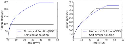
Evolution of bubbles for ambient pressure |$p_0 = 3\times 10^{-12} \, \mathrm{dyne\, cm}^{-2}$| and p0 = 5 × 10⁻¹³dyne cm−2, for average luminosity L = 1.2 × 1037 erg s−1.
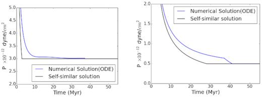
Evolution of pressure inside bubbles for the same cases as in Fig. 2.
The corresponding distribution will be steeper than the self-similar case. This is shown in Fig. 4 for three different epochs. The slopes of the distribution is close to ∼−4, in this particular example, much steeper than −3 in the case of self-similar evolution. The largest bubbles are mostly produced by massive clusters, with large mechanical luminosity, and for which the revised relation for the ambient pressure (equation 5) does not make substantial difference to the bubble size evolution. The number of large bubbles therefore remain more or less the same, whereas the number of smaller bubbles grow to larger sizes than before. This will make the size distribution steeper than the self-similar case.
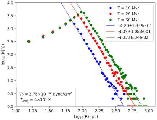
The size distribution of bubbles for adiabatic evolution for an ambient pressure p0 = 2.76 × 10⁻¹² dyne cm−2, at |$10,\, 20,\,\mathrm{\,and\,}30$| Myr. The distributions have a slope ∼−4, much steeper slope than −3 in the case of self-similar evolution. Numerical values of the slopes are indicated in the diagram.
However, the assumption of bubble stalling when pressure equilibrium is reached is not valid, since the bubble shell continues to move outward because of its momentum. This will continue to make the bubbles bigger in size until the outer shock speed becomes comparable to the sound speed of the ambient medium. This can be demonstrated with the help of numerical hydrodynamical simulations, which we describe below.
4 SIMULATION RESULTS
Since the appropriate medium for embedding the superbubbles is the warm neutral medium of ISM, we use namb = 0.5 cm−3 for all our runs (Wolfire et al. 2003). However, we consider the case of different equivalent ISM pressures by assuming different Tamb. It is known that non-thermal pressures in ISM, especially in neutral medium that we are concerned with here, can be substantial (Elmegreen & Scalo 2004) and even more than the thermal pressure. For example, in the solar neighbourhood, Jenkins & Tripp (2011) estimated that turbulent and magnetic pressures are comparable in magnitude, and are roughly three times larger than the thermal pressure. In order to take into account the effect of non-thermal pressure, we use a corresponding equivalent ambient temperature, keeping namb fixed. We use Tamb = 4 × 10⁴ K, for corresponding ISM pressures p0 = 2.8 × 10⁻¹² dyne cm−2 for our fiducial runs, but have also varied the value of Tamb in order to study its influence on size distribution.
Mass and energy are continuously injected within a small radius rc. We use rc = 1 pc, in order to minimize non-physical cooling losses at the early stages of shock formation (see equation 4 in Sharma et al. 2014). According to this criterion, for the lowest luminosity considered here (L = 1036 erg s−1), rc should be less than ≤2.5 pc. Hence the source terms |$S_\mathrm{ m} = \dot{M}/V_\mathrm{ c}$| and Se = L/Vc are non-zero for r < rc, where |$V_\mathrm{ c} = \frac{4\pi }{3}r_\mathrm{ c}^3$|. In the last equation for energy conservation, q− = nineΛ(T), Λ(T) being the cooling function. We have used a tabulated cooling function for solar metallicity. We turn-off cooling when temperature comes down to 104 K, to mimic the effect of photoionization heating in the bubble.
We show the results of simulations with and without cooling in Fig. 5. The luminosities used here is a low value of L = 2 × 1036 erg s−1 (top panels), and a high luminosity of L = 1039 erg s−1 (bottom panels) . The left-hand panels are for Tamb = 4 × 10⁴ K, and the right-hand panels, for Tamb = 2 × 10⁴ K. The self-similar case is show in red, and the result of using equation (5) is shown for comparison in dark blue, although without the condition of stalling at equal pressure. The results of simulations with and without cooling are shown in green and cyan, respectively.
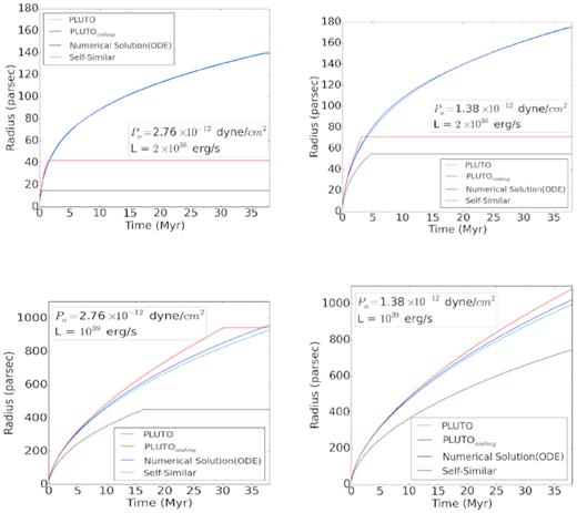
Evolution of radius bubbles from hydrodynamical simulations is compared to the self-similar case. The upper two panels are for L = 2 × 1036 erg s−1 and lower panels, for L = 1039 erg s−1. The left-hand panels show the case for ambient pressure p0 = 2.76 × 10⁻¹² dyne cm−2, and the right-hand panels, for p0 = 1.36 × 10⁻¹² dyne cm−2. Red curves plot the adiabatic self-similar evolution (assuming stalling at pressure equilibrium). Blue curves show the results of using equation (5, assuming stalling at pressure equilibrium). Cyan curves show the results of numerical simulation without cooling, and green curves show the results of simulation with cooling, assuming stalling when outer shock speed equals ambient sound speed.
We first notice that in the case of no radiative cooling (cyan), the evolution of the shell is roughly similar to that of equation (5), except for high mechanical luminosity, in which case the pluto runs give a slightly smaller radius (Fig. 5). This is because of the fact that equation (5) do not take into account mass injection, which is higher in our calculations for higher luminosities (since the wind speed is considered equal in all cases). The injected mass increases the inertia of the shell and decelerates it to some extent.
Secondly, increasing the ambient pressure (without increasing the gas density) makes the bubbles smaller, as expected physically.
4.1 Adiabatic case
Let us first discuss the size distribution in the adiabatic case. As mentioned above, the results of the simulations confirm our analytical results in Section 3, where the pressure gradient term is included in the dynamics of bubbles. We had seen in that case that size distribution is steeper than −3, because of domination of growing bubbles. This is confirmed by the simulation results in which cooling is turned off, and we get a size distribution for the fiducial case with a power-law index ≈−4. The scatter plot of bubbles in this case is shown in Fig. 6 as a function of mechanical luminosity (up to 1037 erg s−1) and bubble age, for a snapshot at 30 Myr. The size of the bubbles are shown in different colours according to the colour palette shown on the right, the red ones being the largest and blue ones being the smallest. It can be seen that the envelopes for different colours (which can be thought of iso-size contours) delineate curves lines in the parameter space. Consider the self-similar case for a moment, in which the combination Lt3 appear together in the relation for size R ∝ (Lt3)1/5. If bubbles were to grow with this scaling, then these envelopes would be curves of t ∝ L−1/3. But these curves in Fig. 6 are more complicated, signifying non-self-similar evolution of bubbles, even in the adiabatic case, because of the presence of pressure gradient term that is neglected in the Weaver et al. (1977) solution.
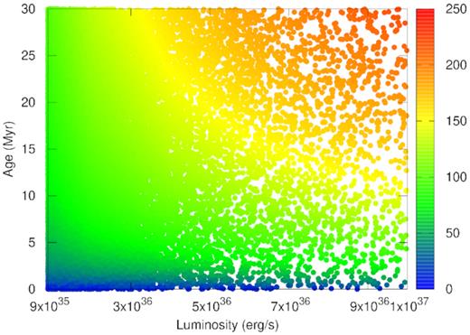
Scatter plot of bubbles in the parameter space of mechanical luminosity L and bubble age, without cooling, after 30 Myr of the onset of star formation, in which the colour of the data points refer to bubble sizes, as shown in the colour palette on the right.
4.2 Effects of cooling
Let us now discuss the effects of cooling. We notice from Fig. 5 that the inclusion of radiative cooling leads to a large difference in the evolution of the shell radius.
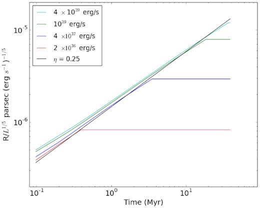
The evolution of the bubbles of different luminosities in the presence of cooling and the pressure difference between ambient and gas inside the bubble, can be roughly described by a single parameter η, which can take into account radiation loss, where η is defined in terms of R = 0.76(ηLt3/ρ)1/5 (the pre-factor |$({250 \over 308 \pi })^{\frac{1}{5}}\approx 0.76$| applies to the adiabatic case Weaver et al. 1977). We show in Fig. 7 the ratio of radius to L1/5 versus time for bubbles of four different luminosities. The curves show that they are nearly superposed on one another, which indicates that a single value of η can describe their evolution, whose value in this case (for the choices of ambient conditions) is inferred to be ∼0.25. Similar conclusions have been reached by previous workers, e.g. Mac Low & McCray (1988) and Krause & Diehl (2014). More recently, Sharma et al. (2014) showed that bubbles can retain a fraction of the input energy, of order 0.2–0.4 depending on ambient conditions (their figs 7 and 8). They also showed that this conclusion is valid even in the presence of thermal conduction. Yadav et al. (2017) further showed that this fraction decreases with increasing ambient density (|$\eta \propto n_{\rm amb}^{-2/3}$|) and is of order |${\sim}20{{\ \rm per\ cent}}$| for ambient density of 0.5 cm−3 (their fig. 8), consistent with our estimate in the present work. Fig. 7 shows that at early epochs, the value of η can vary with luminosity, since the curves for different luminosities do not quite overlap. However, they roughly do so by the time of bubble stalling, which is more relevant to our present work. In general, bubbles with lower luminosity suffer more loss of energy due to radiation (or, η is smaller for lower L), although this trend is reversed below 4 × 1037 erg. This is because of the fact that the outer shock speed is lower for low-luminosity shells, and the resulting post-shock temperature is also reduced, leading to a higher rate of radiative loss, since the cooling function in the relevant temperature range is a decreasing function of temperature. At the lowest luminosities considered here, the post-shock temperature is close to 104 K even at the earliest epochs, where the cooling function drops, reversing the trend.
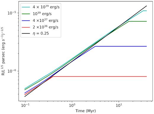
Logarithm of the ratio of radius to mechanical luminosity L in bubbles (in units of cm (erg s−1)−1) is plotted against time (in Myr), for four different values of L, shown in different colours. The ambient pressure is Pamb = 2.76 × 10⁻¹² dyne cm−2, and equivalent temperature is 4 × 10⁴ K. The near superposition of the cases of all luminosities show that a single value of η is able to describe the evolution of bubbles in the presence of radiative cooling. The factor η is found to be ≈0.25, making the bubbles a fraction ≈0.76 times smaller than their adiabatic case.
Scatter plot of bubbles in the parameter space of mechanical luminosity L and bubble age, after 30 Myr of the onset of star formation, in which the colour of the data points refer to bubble sizes, as shown in the colour palette on the right.
We also notice that, as argued previously, bubbles do not stall when pressure inside becomes equal to the ambient pressure. However, the continuation of expansion seen in the simulation is also misleading, because our use of equivalent temperature for non-thermal pressure of the ambient medium has limitations. The non-thermal pressure in the ambient medium due to turbulence and other process will fragment or distort the shell, robbing it of its momentum which would have otherwise make it expand further. This is not easy to simulate without initially introducing density inhomogeneities and turbulence in the ambient medium in the numerical set-up, which would increase the number of free parameters in the calculations. The fact that shells would not be able to retain their identity when their nominal speed becomes comparable to the ambient medium sound speed is self-evident. For example, for SNe blast waves, this was the condition imposed by McKee & Ostriker (1977) in their three phase model of ISM.
Therefore, we impose a condition of stalling the shell when the outer shock speed equals the (isothermal) sound speed of the ambient medium. This is shown by the horizontal section of the green curves in Fig. 5.
5 RESULTS
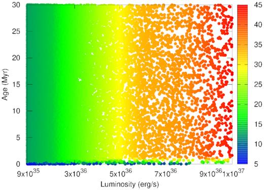
We first show in Fig. 8 a scatter plot of the bubbles as a function of mechanical luminosity (up to 1037 erg s−1) and bubble age, for a snapshot at 30 Myr after the onset of star formation. The bubble sizes being shown in different colours according the colour palette shown on the right, the red ones being the largest and blue ones being the smallest. The SFR is considered to be uniform and equal to 1 M⊙ yr−1, and the luminosity function of clusters is assumed to obey a power law with index β = 2. If we take a snapshot at 30 Myr for bubbles triggered by mechanical luminosity up to 1037 erg s−1, then these are the bubbles that would show up. They will have different ages, as shown by their distribution along the vertical axis. the vertical colour stripes indicate that most bubbles have stalled, being at the same radius at different times, except for the bubbles in the bottom of the figure. This is in contrast to the case without cooling, in which the population of superbubbles is dominated by growing bubbles, in Fig. 6.
The scatter plot shows that at any given time (here, at 30 Myr), the smallest bubbles are produced mostly by low-luminosity clusters (blue circles) and they are predominantly young. This is shown by the fact that blue dots mostly appear at the left bottom corner of this plot. The largest bubbles are created by clusters at the high-luminosity end and can be both young and old. Most of the points in the scatter plot, however, arise due to stalled bubbles. Leaving aside the smallest bubbles (blue), there are vertical columns of different colours (different sizes) in the figure. This implies that the sizes of the bubbles mostly correspond to the mechanical luminosity of the bubbles, and almost independent of the age. This is because of the stalling condition we have imposed at the time of outer shock speed becoming comparable to the ambient medium sound speed.
Fig. 9 shows the relation between final bubble size from our simulations (red points) as a function of mechanical luminosity and shows that the size scales as L1/2. This follows from the fact that radius of a bubble scales as R ∝ (ηL)1/5t3/5, where η ∼ 0.25 takes into account the energy loss by radiation and pressure gradient, as mentioned earlier. This implies an outer shock speed v ∝ (ηL)1/5t−2/5. Since the bubbles are assumed to stall when this speed becomes comparable to the ambient sound speed, the stalling time-scales as ts ∝ L1/2, and consequently, Rf ∝ L1/2.
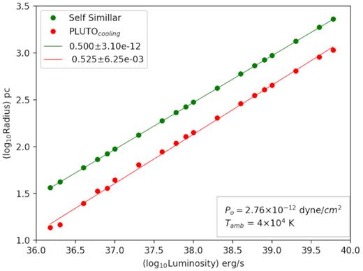
Final bubble size as a function of mechanical luminosity, in the case of self-similar evolution (where stalling is assumed to occur at pressure equilibrium stage, OC97), and from simulations with cooling (in which stalling is imposed when outer shock speed equals the ambient isothermal sound speed).
This stalling condition is similar to that used by OC97, since the ram pressure of the outer shock is related to the pressure of the shocked wind region in a bubble (Weaver et al. 1977), which dominates the pressure inside a bubble. Therefore, it is not a surprise that we get a similar relation between radius and luminosity as in OC97. However, the magnitudes of these two types of pressure are different. The inner pressure is roughly ∼0.8 of the ram pressure (Gupta et al. 2018). Therefore when the inner pressure comes to equilibrium with ambient pressure, the forward shock speed is still higher than the ambient sound speed. The stalling criterion based on speed therefore yields a larger radius by a factor ∼1.2. However when radiative cooling is taken into account, then this criterion gives a smaller radius because of radiation loss.
The second reason why we get a similar scaling between radius and luminosity is the fact that radiation and ambient pressure affects the size evolution through a single factor η, leaving the dependency of size on luminosity the intact. These two facts contrive to make the results in OC97 and in the present work look similar, even in the presence of cooling.
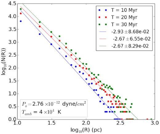
The corresponding size distribution is, therefore, again expected to of the type N(R) ∝ R1 − 2β, and it is shown in Fig. 11. The fitted power-law indices at different epochs (10, 20, 30 Myr) are roughly ∼2.7–2.9. This is close to the value of 1 − 2β(=−3), and the difference from −3 stems from the fact that η weakly depends on luminosity. Had η been totally independent of L, then, the size distribution would have been exactly 1 − 2β(= −3). Since η is somewhat smaller for lower L than its fiducial value, the shells for low-luminosity clusters at stalled phase are somewhat smaller (see equation 11), leading to a somewhat flatter size distribution than the fiducial 1−2β value. Since the radii of bubbles have decreased in general by a factor of 1.7, and the peak radius has decreased by a similar factor compared to the adiabatic case in Fig. 1, to ∼10 pc. While determining the size distribution we did not consider holes smaller than 10 pc, and therefore we do not see any rising part in the distribution with radiative cooling.
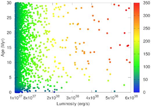
Same as in Fig. 6, but for luminosities in the range 1037–6 × 1038 erg s−1.
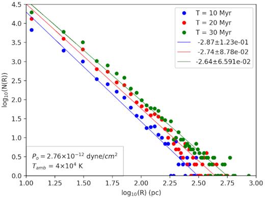
Size distribution of bubbles in our simulation, for ambient pressure p0 = 2.76 × 10⁻¹² dyne cm−2, at 10, 20, and 30 Myr. The distributions at different epochs are fitted with power law, and the power-law indices are found to be ∼2.7.
We show in Appendix A that our results are robust with respect to numerical resolution, although we note that our simulation does not address the issues of turbulence and mixing that may affect radiative losses at different resolutions.
The above results pose question, whether or not one always expects stalled bubbles (and consequently, a size distribution with slope ≈−2.7) in the presence of cooling, or if this depends on the ambient pressure. In order to answer the question, we have run our simulations for two different pressures.
Fig. 12 shows the scatter plot of bubbles (similar to Figs 6 and 8 for our fiducial ISM pressure) for two different values of ISM pressures, at 30 Myr. Essentially, we have decreased the non-thermal contribution in the ambient pressure, by reducing the equivalent temperature from 4 × 10⁴ to 2 × 10⁴ K (left-hand panel) and then to 104 K (right-hand panel). Comparing with Figs 6 (adiabatic case) and 8, we find that the bubbles in these two cases are not dominated by stalled bubbles, as was the case for Fig. 8. For the left-hand panel, we find that bubbles with L ∼ 5 × 1036 erg s−1 stall after a time-scale of ∼7 Myr, and bubbles bigger than that at latter times. When the pressure is further lowered, in the right-hand panel, all bubbles keep growing until 30 Myr, and the circumstance is similar to Fig. 6. We recall that, in these cases of domination by growing bubbles, the size distribution is likely to be steeper than 1 − 2β, as we confirm below.
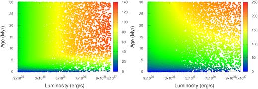
Scatter plot for bubbles for ambient pressure p0 = 1.38 × 10⁻¹² dyne cm−2 (left), and 6.9 × 10⁻¹³ dyne cm−2 (right), at 30 Myr.
We show in Fig. 13 the size distribution of the bubbles for these values of pressure at two different times after the onset of star formation (10 and 30 Myr). In general, we find that lowering pressure steepens the size distribution, by allowing low -luminosity bubbles to grow to larger sizes. This trend is shown in Fig. 14, for two different epochs, 10 and 30 Myr. At lower pressures, there is an evolution of the slope between these time-scales, since bubbles keep growing in low ambient pressure, compared to high-pressure environments.
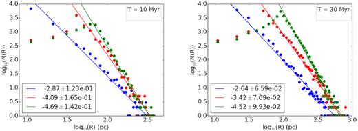
Size distribution of bubbles for ambient pressure p0 = 2.76 × 10⁻¹² dyne cm−2 (blue), 1.38 × 10⁻¹² dyne cm−2 (red), and 6.9 × 10⁻¹³ dynes cm−2 (green), at 10 and 30 Myr.
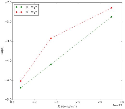
The slope of size distribution as a function of ISM pressure, for two different epochs, 10 Myr (green) and 30 Myr (red).
The distributions at lower (non-thermal) pressures also show a positive part at small sizes, in addition to the falling numbers at large sizes as we have seen earlier. The rising part comes from growing young bubbles whose age is smaller than the stalling time of the bubble with the lowest luminosity. This generates a peak in the distribution. The peak depends upon the radius of the stalled bubble with the lowest luminosity at the time being observed. Fig. 13 shows that at higher pressures the peak radius is independent of time but starts varying with time as soon as we start decreasing the pressure. This occurs due to the fact that at higher pressures (such as, at 2.76 × 10⁻¹² dyne cm−2), the bubbles with low luminosities stall much before 10 Myr hence the peak occurs at the same radius even when we observe the distribution at 30 Myr. However at lower pressures like p0 = 6.9 × 10⁻¹³ dyne cm−2 the bubbles with low luminosities stall much after 30 Myr, and hence the peak shifts towards larger radii with time. In other words, the deviation of the slope from −3 in low-pressure environments indicate evolution of the bubbles, which breaks the relation of L ∝ R2 of stalled bubbles, which would have produced a −3 slope.
6 DISCUSSION
It is known that observations support the 1−2β power law for the superbubble size distribution. For example, Bagetakos et al. (2011) found a power-law index of ≈−2.9 in The HI Nearby Galaxy Survey of 20 nearby galaxies. This is consistent with β ≈ 1.9.
They also reported a variation of the power-law index with galaxy type, with early-type galaxies showing a steeper index (≈4) than late-type galaxies. This indicates, a preponderance of small size holes in early-type galaxies. They associated this phenomenon with the level of star formation activity in different galaxy types. One obvious connection is that in early-type galaxies, the observed mass function of star clusters is steeper than late-type galaxies, as evidenced by the H ii region luminosity function (e.g. Kennicutt, Edgar & Hodge 1989). While the luminosity function in Sb–Sc galaxies has an index of ∼−2, the index varies from ∼−1.7 in Sc−Im galaxies (Banfi et al. 1993) to ∼2.6 in Sa galaxies (Caldwell et al. 1991). Oey & Clarke (1998) explained this variation in the H ii region luminosity function in terms of a truncation in the maximum value of the luminosity distribution that depends on Hubble type. This corresponds to early-type galaxies having a maximum cluster mass that is much lower than for late-type galaxies.
We mention in passing that it is also possible that lower SFR in early-type galaxies would lead to lower non-thermal pressure, as has been seen in simulations (Joung, Mac Low & Bryan 2009). According to their results, the turbulent pressure scales with surface density of star formation as |$P_{\rm turb} \propto \Sigma _\ast ^{2/3}$|. Since our results indicate that decreasing non-thermal pressure steepens the size distribution, this remains another possibility. Future observations will be able to point towards the right explanation.
We note that our calculations do not take into account the merging of superbubbles and its effect on the size distribution. This was discussed by OC97 in terms of a porosity parameter Q (Cox & Smith 1974), which is the ratio of superbubble volume to total ISM volume. For the Milky Way, the SFR is near the critical point where Q ∼ 1. It can be shown that the total volume occupied by superbubbles can exceed the volume of Milky Way ISM, considering a cylinder of 10 kpc radius and 500 pc thickness, within ≤1 Myr, if the SFR is assumed to be ∼3 M⊙ yr−1. Following Clarke & Oey (2002), if one takes the average mass of clusters as ∼1300 M⊙, then the number of superbubbles produced per Myr is ∼2200, for an SFR of 3 M⊙ yr−1. Then with a size distribution with a slope of −3, the total volume exceeds the Milky Way ISM volume in ≤1 Myr. This is also supported by the estimates of Krause et al. (2015). At the same time, the observed volume filling factor of H i shells in the Milky Way is less than |${\sim}10{{\ \rm per\ cent}}$| (Bagetakos et al. 2011). This implies that merging of superbubbles is important. It is also evident from the observations of Simpson et al. (2012) that roughly |${\sim}30{{\ \rm per\ cent}}$| of H i shells show signs of merging. OC97 also explore how the Milky Way Q varies with the assumed value of β. Merging among superbubbles likely flattens the size distribution to some extent, by increasing the number of large bubbles at the expense of smaller bubbles. However, it is difficult to estimate the magnitude of this effect without a simulation that includes non-uniformity in the spatial distribution of star clusters.
7 CONCLUSIONS
We have studied the form and evolution of the size distribution of H i holes in the ISM of galaxies owing to superbubbles triggered by OB associations, taking into account radiative cooling, with the help of numerical hydrodynamical simulations. Previous works had assumed bubble growth stalls when the inner pressure of adiabatic bubbles equals the ambient pressure, which is not valid since the bubbles maintain momentum-driven growth. Assuming that bubbles stall when the expansion speed becomes comparable to the ambient sound speed, we show that the inclusion of radiative cooling and ambient pressure results in a power-law index of the size distribution with slope ∼−2.7 for an ISM pressure of p0 = 2.8 × 10⁻¹² dyne cm−2 and density n = 0.5 cm−3. This is consistent with observations by THINGS. We have further shown that decreasing the ISM pressure can make the population of growing bubbles dominating over stalled ones, consequently making the size distribution steeper. Our results imply that the size distribution can help interpret the evolution of bubbles, with the slope being ∼−2.7 in the case of domination by stalled bubbles, and with a steeper slope for the case of growing bubbles. We have discussed the possibility that the size distribution in early-type galaxies is steeper than late-type galaxies because of the difference in the intrinsic luminosity function as a function of galaxy type. A steeper luminosity function of star clusters in late-type galaxies leads to a steep size distribution, as observed.
ACKNOWLEDGEMENTS
We would like to thank K. S. Dwarakanath, Nirupam Roy, Aditi Vijayan, Siddhartha Gupta, and Ranita Jana for useful discussions. The authors thank the anonymous referee for helpful comments. PD would like to thank Raman Research Institute for local hospitality during her visits for the project.
REFERENCES
APPENDIX A: CONVERGENCE TEST
Here, we present the convergence tests of the numerical runs for superbubble evolution for our fiducial case, for a different spatial resolution, with Δr = 0.1 pc, instead of 0.16 pc used earlier. Fig. A1 shows the size distribution and fitted slopes at 10, 20, and 30 Myr, for the fiducial case of P0 = 2.76 × 10⁻¹² dyne cm−2. The slopes (−2.93, −2.67, −2.67) are similar to the ones (−2.87, −2.74, −2.64) obtained for a coarser resolution (Fig. 11). This confirms the convergence of our results with respect to numerical resolution.
Similar to Fig. 11 except that it is for Δr = 0.1 pc.
This implies that η has also reached convergence limit, and we show in Fig. A2 the logarithm of ratio of radius to L1/5 versus time for different luminosities, superimposed on the expected evolution for η = 0.25. The curves show (as in Fig. 7) that η depends on luminosity rather weakly.
Similar to Fig. 7 except that this is for Δr = 0.1 pc.
We should note that our runs do not simulate the effects of turbulent mixing in ISM, which might render numerical convergence ineffective (e.g. Gentry et al. 2019; Fierlinger et al. 2016). However, those effects are beyond the scope of the present work.
