


ABSTRACT
Most ultraluminous X-ray sources (ULXs) are thought to be powered by neutron stars and black holes accreting beyond the Eddington limit. If the compact object is a black hole or a neutron star with a magnetic field ≲1012 G, the accretion disc is expected to thicken and launch powerful winds driven by radiation pressure. Evidence of such winds has been found in ULXs through the high-resolution spectrometers onboardXMM–Newton, but several unknowns remain, such as the geometry and launching mechanism of these winds. In order to better understand ULX winds and their link to the accretion regime, we have undertaken a major campaign with XMM–Newton to study the ULX NGC 1313 X-1, which is known to exhibit strong emission and absorption features from a mildly relativistic wind. The new observations show clear changes in the wind with a significantly weakened fast component (0.2c) and the rise of a new wind phase which is cooler and slower (0.06–0.08c). We also detect for the first time variability in the emission lines which indicates an origin within the accretion disc or in the wind. We describe the variability of the wind in the framework of variable super-Eddington accretion rate and discuss a possible geometry for the accretion disc.
1 INTRODUCTION
Ultraluminous X-ray sources (ULXs) are bright, point-like, off-nucleus, extragalactic sources with X-ray luminosities above 1039 erg s−1 that result from accretion on to a compact object (see e.g. Kaaret, Feng & Roberts 2017). Recent studies have shown that some ULXs are powered by accretion on to neutron stars with strong magnetic fields (1012–14 G, e.g. Bachetti et al. 2014; Fürst et al. 2016; Tsygankov et al. 2016; Israel et al. 2017a, b; Brightman et al. 2018; Carpano et al. 2018; Middleton et al. 2019; Rodriguez Castillo et al. 2019; Sathyaprakash et al. 2019). Moreover, since more than a decade it has been thought that the majority of ULXs consists of stellar-mass compact objects (<100 M⊙) at or in excess of the Eddington limit (King et al. 2001; Poutanen et al. 2007; Gladstone, Roberts & Done 2009; Liu et al. 2013; Middleton et al. 2013; Motch et al. 2014). In particular, the presence of a strong turnover below ∼7 keV in most ULX (and all NuSTAR) spectra (see e.g. Gladstone et al. 2009; Bachetti et al. 2013; Walton et al. 2018) and the simultaneous high 1039–41 erg s−1 luminosities are difficult to explain with sub-Eddington accretion models.
However, some ULXs might still host more massive black holes (|$10^{2-5} \, \mathrm{M}_{\odot}$|) at more sedate Eddington ratios (see e.g. Greene & Ho 2007; Farrell et al. 2009; Webb et al. 2012; Mezcua et al. 2016).
At accretion rates approaching the Eddington limit, radiation pressure inflates the thin disc, producing a geometry similar to that of a funnel and a wind is launched (see e.g. Shakura & Sunyaev 1973; Poutanen et al. 2007). Winds driven by radiation pressure in a super-Eddington (or supercritical) regime can reach mildly relativistic velocities (∼0.1c, see Takeuchi, Ohsuga & Mineshige 2013) and therefore may carry a huge amount of matter and kinetic energy out of the system. They can affect the accretion on to the compact object and the physical state of the nearby interstellar medium by inflating large (∼100 pc) bubbles. For a quantitative comparison between the wind power and the energetics of the bubbles see Pinto et al. (2020) and references therein.
Evidence for such winds was first seen through strong residuals at soft X-ray energies (< 2 keV) to the best-fitting models describing the continuum of ULXs, albeit unresolved, in the low-to-moderate resolution CCD spectra (see e.g. Stobbart, Roberts & Wilms 2006). The time variability of such residuals and its correlation with the source spectral hardness suggested that they might be produced by the ULX itself and possibly in the form of a wind (see e.g. Middleton et al. 2014; Middleton et al. 2015b).
Finally, our team (Pinto, Middleton & Fabian 2016) identified strong (>5σ) rest-frame emission and blueshifted (∼0.2c) absorption lines in the high-resolution X-ray spectra of two bright ULXs, namely NGC 1313 X-1 and NGC 5408 X-1, taken with the XMM–Newton Reflection Grating spectrometer (RGS). Walton et al. (2016a) found a Fe K component to the outflow in NGC 1313 X-1 significant at the 3σ level through the combination of hard X-ray spectra taken with XMM–Newton and the Nuclear Spectroscopic Telescope Array(NuSTAR; Harrison et al. 2013). Additional evidence of powerful winds was found in the RGS spectra of other sources such as the soft NGC 55 ULX (Pinto et al. 2017) and the intermediate hardness NGC 5204 ULX-1 (Kosec et al. 2018a). Recently, Wang, Soria & Wang (2019) found evidence of blueshifted emission lines in Chandra and XMM–Newton spectra of a transient ULX in NGC 6946. The first discovery of outflows in the ultraluminous X-ray pulsar NGC 300 PULX (Kosec et al. 2018b) showed that strong magnetic fields (e.g. |$\sim 10^{12}\, \mathrm{G}$|) and winds can coexist as is also shown by the theoretical calculation of Mushtukov et al. (2019).
In the last decade, a unification scenario for ULXs has gained popularity, which proposes that the observed behaviour from ULXs (i.e. broad-band spectra, variability properties) depends on both their accretion rates and viewing angles (see e.g. Poutanen et al. 2007; Middleton et al. 2015a; Feng et al. 2016; Urquhart & Soria 2016; Pinto et al. 2017). Moreover, we should expect higher ionization states in the wind at low inclinations (on-axis) due to exposure to harder SEDs in the inner regions of the disc (Pinto et al. 2020). The study of the winds provides an alternative and complementary tool to understand the physics of ULXs and super-Eddington accretion to the modelling of the broad-band spectral continuum.
Despite important discoveries and the progress on ULXs in the last decade, several problems are still to be solved: How does the wind vary with the accretion rate? What is the geometry and the ionization structure of the wind? What is the launching mechanism? What is its energy budget? Can the wind affect the ULX surroundings and the accretion of matter on to the compact object? If the compact object is a magnetized neutron star, could a strong magnetosphere disrupt the disc and suppress the wind? When and how jets are launched in ULXs?
In order to place some constraints on these unknowns we were awarded 6 orbits targeting the NGC 1313 galaxy with XMM–Newton during AO16 (PI: Pinto) and obtained quasi-simultaneous NuSTAR coverage of the hard X-ray band (PI: Walton) for some observations. Additional observations were taken with Chandra (PI: Canizares). This is the first paper in a series focusing on NCG1313 X-1, and presents a study of its wind as seen by XMM–Newton and, in particular, its variability with the ULX spectral state. Detailed broad-band spectroscopy and the analysis of the NuSTAR data is performed in Walton et al. (2019), while the search for narrow spectral lines in the hard band with the Chandra gratings (HETGS) will be shown in Nowak et al. (in preparation). Our campaign has already provided important results such as the first discovery of pulsations in the NGC 1313 X-2 (Sathyaprakash et al. 2019), which added a new PULX candidate to a list which includes only a handful of sources at the present. We also report the discovery of a soft X-ray lag in new XMM–Newton data of NGC 1313 X-1 from this campaign in a companion paper (Kara et al. 2020). Soft lags were discovered only in two other ULXs.
We detail our campaign in Section 2 and show the spectral analysis in Section 3. In Section 4, we show the principal component analysis (PCA). We discuss the results in Section 5 and give our conclusions in Section 6. Throughout the paper we use C-statistics (Cash 1979), adopt 1 σ error bars and perform the spectral analysis with the spex code1 (Kaastra, Mewe & Nieuwenhuijzen 1996).
2 THE DATA PRODUCTS
2.1 NGC 1313 X-1 archival data
NGC 1313 X-1 is an archetypal bright ULX (|$L_{\, 0.3-10\, {\rm keV}}$| up to ∼1040 erg s−1). Its relatively small distance (D = 4.2 Mpc, e.g. Tully et al. 2013) makes it a good target for the high-spectral-resolution RGSs aboard XMM–Newton, which cover the 0.3–2 keV energy band where strong (unresolved) features were found in low-spectral resolution CCD spectra (Middleton et al. 2015b). The strength of these features decreases at higher luminosity and spectral hardness (they define as hardness the ratio of the unabsorbed 1–10/0.3–1 keV fluxes, while in this paper we use the standard 2–10/0.3–2 keV flux ratio, so our brightest states are also the softest). The RGS spectra resolve the spectral features in a forest of rest-frame emission lines and relativistically blueshifted (∼0.2c) absorption lines from a wind as shown by Pinto et al. (2016). In that paper, high-spatial resolution Chandra maps indicate that the X-ray emission is confined to a circular region of a few arcseconds, confirming that the residuals are intrinsic to the ULX as shown by Sutton, Roberts & Middleton (2015) and Sathyaprakash, Roberts & Siwek (2019) for NGC 5408 X-1 and Holmberg IX X-1.
XMM–Newton has observed the NGC 1313 galaxy before our campaign for 25 times with exposures ranging from 9 (snapshot) to 137 ks (full orbit). However, of these observations, only three had ULX-1 on-axis for a significant amount of time and with an appropriate roll angle.
Kosec et al. (2018a) have shown that observations of about 100 ks are normally required to detect and resolve strong lines in ULX RGS spectra. Moreover, RGS observations have to be performed with accurate pointing (on-axis) and roll angle in order to avoid contamination from any other bright source located along the (long) dispersion direction axis of the RGS field of view (FOV; ∼5 arcmin × 30 arcmin).
In Table 1, we provide some essential information on the deepest observations of NGC 1313 X-1 (on-axis) taken with XMM–Newton. The three old observations (2006 October and 2012 December) are the same used in Pinto et al. (2016) and Walton et al. (2016a). The two following observations (2014 July, 2017 March) provide a sufficient amount of exposure time, but the roll angle is not optimal since the RGS selection region for ULX-1 intercept either ULX-2 or the supernova remnant SN 1978K. These two observations are therefore not used in our high-spectral-resolution analysis.
XMM–Newton observations used in this paper.
| OBS_ID | Date | State | Flux | tRGS1, 2 | tpn | tMOS1 | tMOS2 | Notes | Stacking |
|---|---|---|---|---|---|---|---|---|---|
| (|$\rm {photons \, m}^{-2}\, \rm {s}^{-1}$|) | (ks) | (ks) | (ks) | (ks) | group | ||||
| 0405090101 | 2006-10-15 | Low–Int | 7.8 | 97 | 81 | 99 | 99 | OLD L–I | |
| 0693850501 | 2012-12-16 | Low–Int | 10.1 | 112 | 90 | 114 | 113 | OLD L–I | |
| 0693851201 | 2012-12-22 | Low–Int | 11.0 | 117 | 85 | 122 | 121 | OLD L–I | |
| 0742590301 | 2014-07-05 | Int–Bright | 18.1 | 62 | 54 | 61 | 61 | (*) | |
| 0794580601 | 2017-03-29 | Low–Int | 11.0 | 41 | 26 | 39 | 37 | (*) | |
| 0803990101 | 2017-06-14 | Int–Bright | 15.5 | 131 | 109 | 128 | 128 | NEW I–B | |
| 0803990201 | 2017-06-20 | Int–Bright | 13.5 | 130 | 111 | 129 | 128 | NEW I–B | |
| 0803990301 | 2017-08-31 | Low–Int | 8.6 | 109 | 42 | 70 | 64 | (**) | NEW L–I |
| 0803990401 | 2017-09-02 | Low–Int | 8.5 | 115 | 53 | 50 | 46 | (**) | NEW L–I |
| 0803990701 | 2017-09-24 | Low–Int | 9.1 | 121 | 11 | 10 | 10 | (***) | NEW L–I |
| 0803990501 | 2017-12-07 | Int–Bright | 12.0 | 90 | 60 | 89 | 86 | (**) | NEW I–B |
| 0803990601 | 2017-12-09 | Int–Bright | 14.7 | 109 | 71 | 117 | 116 | (**) | NEW I–B |
Notes. The ULX state refers to the low-to-intermediate and intermediate-to-bright flux levels, primarily chosen from the total flux and shape of the X-ray spectra (see Figs 2 and A1). Absorbed 0.3–10 keV fluxes are computed with a multicomponent model consisting of two modified blackbody components plus comptonization corrected for Galactic absorption (see Section 3.1). Exposure times account for background flaring removal. (*) RGS spectra contaminated by either X-2 or SNR (only EPIC-pn is used for PCA); (**) EPIC cameras affected by solar flares; (***) Additional calibration exposure (only RGS is operating for the full orbit).The acronyms OLD L–I, NEW L–I, and NEW I–B stay for old low–intermediate, new low–intermediate, and new intermediate–bright states.
2.2 NGC 1313 X-1 XMM–Newton campaign
We observed the NGC 1313 galaxy in 2017 with a deeper campaign led by XMM–Newton. The roll angle was chosen to avoid any contamination along the dispersed RGS spectra from the two nearby brightest X-ray sources (ULX-2 and SN 1978K, see Fig. 1). In addition, we observed the source in three different epochs separated by 2–3 months during 2017. The primary goals were (a) to detect the source in different spectral states and (b) to study the variability of the wind according to the spectral state.
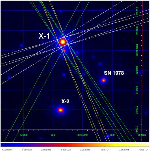
XMM–Newton image of the NGC 1313 field obtained by combining all the data available from EPIC-pn and MOS 1,2. The green, yellow, and white dashed lines indicate the RGS extraction region for the old Low–Int, new Low–Int, and new Int–Bright spectra, respectively (see notation in Table 1). The other ULX (X-2) and the supernova remnant (SN 1978) are also labelled. The apparent lower number of data sets is due to the fact that some pointings have the same average position angles.
The choice of the time windows was dictated by the historical light curve of NGC 1313 X-1 taken with the Neil Gehrels Swift Observatory (hereafter Swift; Gehrels et al. 2004), which shows long-term variability on time-scales of 2–3 months (see Fig. 2). Such variability is of crucial importance as an ∼ 60 d modulation has been detected in some ULXs and interpreted as the orbital or the superorbital period of the binary system (see e.g. Kaaret, Simet & Lang 2006; Motch et al. 2014; Walton et al. 2016b; Fürst et al. 2018; Brightman et al. 2019). Observations of NGC 1313 X-1 separated by 2–3 months may therefore provide insights on the geometry of the ULX system and the complex structure of the wind. More detail on the analysis of the Swift observations and the long-term variability of NGC 1313 X-1 will provided elsewhere (Middleton et al. in preparation).
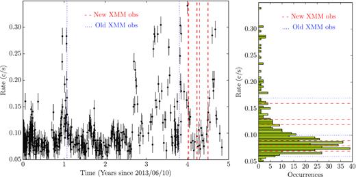
Left: Long-term Swift/XRT light curve of NGC 1313 X-1 with the dates of the XMM–Newton observations indicated by dotted (old) and dashed (new, 2017) lines. Right: Corresponding count rate histogram with the XMM–Newton observations indicated.
The observations of NGC 1313 X-1 were therefore divided in three groups each consisting of a pair of full orbits within a few days of each other in order to obtain a combined, deep (≳200 ks), RGS spectrum of the ULX representative of a specific flux regime or accretion rate.
In addition to the 6 orbits awarded during AO16, one additional orbit was awarded to perform EPIC calibration. During this observation, only RGS and OM could be operated for the full duration of the observation, while the CCD cameras (pn and MOS 1,2) were active for only approximately 10 ks each. We also use these observations, but their CCD data have limited statistical weight.
2.3 NuSTAR and Chandra follow-up
Details of the NuSTAR archival and follow-up observations are given in Table 2. We also report whether the observations were simultaneous to XMM–Newton or Chandra. The Chandra observations taken throughout 2017 accumulate up to 500 ks of exposure time, but each is relatively short (between 10 and 50 ks). In this paper, we only use the NuSTAR time-averaged spectrum to cover the high-energy (>10 keV) range to build-up our broad-band spectral energy distribution (SED) and perform accurate photoionization modelling.
NuSTAR observations used in this paper.
| OBS_ID | Date | tFMPA, B | Notes |
|---|---|---|---|
| (ks) | |||
| 30002035002 | 2012-12-16 | 154 | (*) |
| 30002035004 | 2012-12-21 | 206 | (*) |
| 80001032002 | 2014-07-05 | 73 | (*) |
| 90201050002 | 2017-03-29 | 125 | (*) |
| 30302016002 | 2017-06-14 | 100 | (**) |
| 30302016004 | 2017-07-17 | 87 | (***) |
| 30302016006 | 2017-09-03 | 90 | (**) |
| 30302016008 | 2017-09-15 | 108 | (***) |
| 30302016010 | 2017-12-09 | 100 | (**) |
Notes. (*, **) archival and new observations simultaneous with XMM–Newton, (***)new observations simultaneous with Chandra. All exposures are given to the nearest ks.
2.4 Data reduction
In this work, we use data from the broad-band European Photon-Imaging Camera (EPIC; Turner et al. 2001) and the RGS (den Herder et al. 2001) aboard XMM–Newton as well as the two focal plane modules (FPMA/B) aboard NuSTAR (Harrison et al. 2013).
The primary science is carried out with the RGS which can detect and resolve narrow spectral features. The broad-band cameras (EPIC and FPMA/B) are mainly used to provide the correct spectral continuum and cover the hard X-ray band which is not covered by the RGS. The EPIC count rate is much higher than RGS in the soft (|$\lt \, 2$| keV) band. However, the energy resolution of the EPIC CCD cameras is insufficient to resolve narrow features, particularly in the soft band (|$R_{\, 0.3-2 \, \rm keV, \, pn}=\Delta E/E \sim 10\!-\!20$|). Therefore, we only use the EPIC-pn spectrum between 2 and 10 keV. Below 2 keV, we only use RGS data (|$R_{\, 0.3-2 \, \rm keV, \, RGS}=\Delta E/E \sim 100\!-\!600$| for the first-order spectra). We have decided not to use the MOS 1,2 cameras for spectroscopy but just for imaging as each has 3–4 times less effective area (and even less above 8 keV) than pn. Moreover, we mainly use broad-band spectra to constrain the continuum shape and minimize its effects on to the RGS line search.
The NuSTAR data are only used here between 10 and 20 keV to cover the hard X-ray band and determine the source continuum. This choice is dictated by the fact that (1) only a few NuSTAR and XMM–Newton observations are fully simultaneous and (2) we want to maximize the statistical weight of the high-resolution RGS spectra. A detailed and in-depth analysis of the NuSTAR data are presented in Walton et al. (2019). Here, we briefly give the main steps of the data reduction and the production of the time-averaged NuSTAR spectrum. We reduce the NuSTAR data with the NuSTAR Data Analysis Software (nustardas v1.8.0 and caldb v20171204). The unfiltered event files are cleaned with nupipeline. We adopt the standard depth correction, which significantly reduces the internal background at high energies, and periods of Earth-occultation and passages through the South Atlantic Anomaly are also excluded. Source products are extracted from circular regions of radius 30 arcsec and the background is estimated from a larger square in a nearby region of the same detector free of contaminating point sources. Spectra and light curves are extracted from the cleaned event files using NUPRODUCTS for both focal plane modules (FPMA and FPMB). In addition to the standard ‘science’ data (mode 1), we also extract the ‘spacecraft science’ data (mode 6) following Walton et al. (2016c). Finally, all NuSTAR spectra are combined into a single time-averaged spectrum using the FTOOL ADDASCASPEC.
We reduce the 12 XMM–Newton observations with the sas2 v16.0.0 (caldb available on 2019 February). Briefly, EPIC-pn, MOS, and RGS data are reduced with the epproc, emproc, and rgsproc tasks, respectively, to produce calibrated event files, spectra response matrices and images. Following the standard procedures, we filter the MOS and pn event lists for bad pixels, bad columns, cosmic ray events outside the FOV, photons in the gaps (FLAG = 0), and apply standard grade selection, corresponding to PATTERN ≤12 for MOS and PATTERN ≤4 for pn. We correct for contamination from soft-proton flares through the sas task evselect by selecting background-quiescent intervals on the light curves for MOS 1, 2, and pn in the 10–12 keV energy band, while we use the data from the CCD number 9 for RGS (corresponding to ≲7.5 Å or ≳1.7 keV). The light curves are grouped in 100 s intervals and all the time bins with a count rate above 0.4 c s−1 are rejected for pn, 0.2 c s−1 for both MOS and RGS. We build the good time interval (GTI) files with the accepted time events for the pn, MOS, and RGS data through the sas task tabgtigen and filter the data with these GTI files. For RGS 1 and 2, we join the GTI and obtain the same exposure times. The RGS 1-2, MOS 1-2, and pn total clean exposure times are quoted in Table 1.
Solar flares significantly affected the EPIC data throughout the low-flux observations of our campaign for about 50 per cent of the exposure time. Fortunately, solar flares affect the RGS data on a much lower level. We extract EPIC MOS 1–2 and pn images in the 0.3–10 keV energy range and stack them with the emosaic task (see Fig. 1). We also extract EPIC-pn spectra from within a circular region of 30 arcsec radius centred on the emission peak. The background spectra are extracted from within a larger box in a nearby region on the same chip, but away from bright sources and the readout direction (see Fig. 1). We also make sure that the background region is not placed in the copper emission region (Lumb et al. 2002).
We extract the first-order RGS spectra in a cross-dispersion region of 0.8 arcmin width, centred on the emission peak, and the background spectra by selecting photons beyond the 98 per cent of the source point spread function, making sure that the background regions do not overlap with either X-2 or SN 1978, and check for consistency with blank field data.
2.4.1 Spectral states of NGC 1313 X-1
The EPIC-pn spectra of NGC 1313 X-1 are shown in Fig. A1. It is clear that our observing strategy was appropriate because it enabled us to recovered a broad and continuous range of spectra ranging from the low flux to very bright states (or hard ultraluminous and broadened disc, e.g. Sutton, Roberts & Middleton 2013). The archival observations provide further useful information and fill some small flux gaps in our new exposures (Fig. A1). It is not strictly accurate to speak of individual spectral states as the source does not jump from one to another but rather moves smoothly among them. However, in order to simplify the terminology, we still refer to low-to-intermediate (hard) and intermediate-to-bright (broadened-disc) states (see also Table 1). For instance, the other ULX in the same galaxy, NGC 1313 X-2, seems to switch between two preferred states (see e.g. Weng & Feng 2018), perhaps due to some processes related to the presence of strong magnetic fields from the neutron star recently discovered (Sathyaprakash et al. 2019).
In order to better understand our spectra and place them within the context of the source variability, we extract the historical light curve of NGC 1313 X-1 as obtained by Swift/XRT using the website tool3 (Evans et al. 2009) which processes the data with heasoft v6.22. In Fig. 2 (left), we show the Swift/XRT light curve from 2013 June where good sampling with intervals of a few days was available. The source has shown a remarkable activity in the last 2 yr if compared to previous periods of time (more detail on the long-term behaviour will be provided by Middleton et al. in preparation). The XMM–Newton observations were taken towards the end of a bright period (middle 2017 June), during the central part of its low-flux time range (early September) and finally in the beginning of the new rise (early December). Fig. 2 (right) shows the histogram of the count rate taken from the Swift/XRT light curve with the dashed-red and dotted-blue lines indicating the flux levels of the new and archival XMM–Newton observations, respectively. These flux levels are interpolated between the two closest Swift points in the light curve and provide rough approximations of the actual levels, useful to place the XMM–Newton observations in the general context of long-term source variability.
2.4.2 Flux-/time-resolved spectra
We stack the first-order RGS 1 and 2 spectra from the observations with a similar flux level and spectral state (either archival/old low-to-intermediate, or new low-to-intermediate or new intermediate-to-bright) with the task rgscombine (see Table 1). Similarly, we stack the EPIC-pn spectra for the archival and the new observations using epicspeccombine. The NuSTAR data are used mainly to cover the hard band and, since there is no major variability above 10 keV during our campaign and in the archival spectra used in this paper (Walton et al. 2019), we prefer to stack all NuSTAR FPMA,B spectra into a single deep spectrum and use only the data points between 10 and 20 keV. We remind the reader that the wind search is driven by the high-resolution RGS spectra. In summary, for the spectral analysis in this paper, we will focus on three pairs of simultaneous XMM–Newton/RGS (0.4–2 keV) and EPIC-pn (2–10 keV) deep spectra and one NuSTAR (10–20 keV) spectrum.
The flux–resolved RGS and EPIC spectra are shown in Fig. 3. The top panel shows the archival XMM–Newton RGS-EPIC spectrum that was also used in Pinto et al. (2016). This spectrum shows the canonical low-to-intermediate flux hard ultraluminous state according to the classification of Sutton et al. (2013). Well-known rest-frame emission (and blueshifted absorption) lines are labelled with solid red (dotted/dashed blue) lines. The middle panel shows the low-to-intermediate flux spectrum taken during our new XMM–Newton campaign. The spectrum is indeed very similar to the archival spectrum. However, it is clear that some features have weakened (if not disappeared) while some new ones show up in the new spectrum. Some emission lines, in particular, seem to have strengthened. This suggests long-term temporal variability of the wind and provides another reason to avoid the stacking of the old data set with the new low–intermediate data. This is even more obvious in the high-state (intermediate-to-bright) spectrum of our campaign (bottom panel in Fig. 3) where most emission lines appear stronger and broader than in the low state spectra.
![Flux-resolved XMM–Newton RGS (0.45–2 keV), EPIC-pn (2–10 keV), and NuSTAR (10–20 keV) spectra. The top panel shows the RGS and pn spectra obtained by stacking the archival data (see also Pinto et al. 2016). The middle panel shows the stacked spectra produced using the low-to-intermediate flux observations of our 2017 campaign (ID: 0803990301, 0401, 0701). The bottom panel shows the stacked spectra produced using the new intermediate-to-high flux observations (ID: 0803990101, 0201, 0501, 0601); see also Table 1. The range between 10 and 20 keV is covered by the time-averaged NuSTAR spectrum. The red lines show the baseline continuum models [hot(mbb + mbb + comt), see Table 3]. The strongest emission lines are indicated with solid red labels. Previously known and confirmed absorption features are indicated with dotted blue lines. New possible features are shown as dashed light-blue lines.](https://oup.silverchair-cdn.com/oup/backfile/Content_public/Journal/mnras/492/4/10.1093_mnras_staa118/1/m_staa118fig3.jpeg?Expires=1750675721&Signature=Yjhj7F-jZb07TSh8OoXzHqp3ZaENIkYJExMIV5YQEOtyD2~ysg8MRgkjRuAsV32ydY7pzVWSzoCBtjKydGq-FKSRlgZr5RjkH1CGVATN3pPVX7jNjhMuVPiZFdNFtB1VsIDebHw~LOn4gkfIOLzzEshasYPmyqCNB0Lu77e~vJcCU01h6yj329WR3JmsZFjWeFgHfOIGl0qiyGoSHo29l8mitgPXqx6Cofo86S7Dg0c2pizTvXP8Kfk-LzeCGQzE~GHZNNXzKb4ZhDFgPbCf1X6panqJVE0sXK~EljQqxNdLNx9GymWPqxDv7LZJZxUXas549THboYzqss8sroYwAQ__&Key-Pair-Id=APKAIE5G5CRDK6RD3PGA)
Flux-resolved XMM–Newton RGS (0.45–2 keV), EPIC-pn (2–10 keV), and NuSTAR (10–20 keV) spectra. The top panel shows the RGS and pn spectra obtained by stacking the archival data (see also Pinto et al. 2016). The middle panel shows the stacked spectra produced using the low-to-intermediate flux observations of our 2017 campaign (ID: 0803990301, 0401, 0701). The bottom panel shows the stacked spectra produced using the new intermediate-to-high flux observations (ID: 0803990101, 0201, 0501, 0601); see also Table 1. The range between 10 and 20 keV is covered by the time-averaged NuSTAR spectrum. The red lines show the baseline continuum models [hot(mbb + mbb + comt), see Table 3]. The strongest emission lines are indicated with solid red labels. Previously known and confirmed absorption features are indicated with dotted blue lines. New possible features are shown as dashed light-blue lines.
All XMM–Newton and NuSTAR spectra are sampled in channels of at least 1/3 of the spectral resolution, for optimal binning and to avoid oversampling, and at least 25 counts per bin, using sas task specgroup. However, all stacked spectra have long exposure times and high quality, which means that such binning affects only the spectral range at the very low and high energies. We have double checked and found no effect on to our line or continuum modelling by decreasing the binning to simply 1/3 of the spectral resolution.
3 SPECTRAL ANALYSIS
In this section, we present the spectral analysis of NGC 1313 X-1. We first show the baseline, continuum, model that describes the broad-band (0.4–20 keV) spectrum. Then we perform an in-depth analysis of the high-resolution RGS spectra in order to detect strong sharp features and to search for variability in the line strength between different spectral states and epochs. We then build-up self-consistent models of gas in photoionization and collisional ionization equilibrium to study the ionization and dynamical structure of the wind responsible for both emission and absorption lines.
3.1 Baseline continuum model
ULX spectra require several components to obtain a satisfactory description of the continuum. Here, we adopt a broad-band spectral continuum similar to that one used in Walton et al. (2018). Two modified blackbody components, mbb1, 2, account for the outer and inner disc; a comptonized component comt describes the hard tail (see also Middleton et al. 2015a). All emission components are corrected by absorption due to the foreground interstellar medium and circumstellar medium using the hot model in spex with a low temperature 0.5 eV (e.g. Pinto et al. 2013). In the spectral fits, we couple the column density of the hot model across all observations as we do not know physical reasons for which the amount of neutral gas should significantly change on time-scales of a few days. Moreover, a preliminary spectral fit performed with free column densities in the three spectra using the mbb1, 2 + comt model yields consistent column densities.
We apply the hot(mbb + mbb + comt) continuum model to the three flux-resolved spectra that we have defined and produced in Section 2.4.2. This phenomenological model provides a good description of the three broad-band spectra. The results are shown in Fig. 3 and Table 3. We obtain an average column density of NH = (1.9 ± 0.1) × 1021 cm−2, which is close to the value of (2.5 ± 0.1) × 1021 cm−2 measured for different continuum models in Walton et al. (2019); see also Miller et al. (2013).
Best-fitting broad-band continuum models.
| Parameter | OLD L–I | NEW L–I | NEW I–B |
|---|---|---|---|
| Baseline model : |$hot\, (mbb+mbb+comt)$| | |||
| |$L_{X\, mbb1}$| | 3.1 ± 0.4 | 2.4 ± 0.3 | 5.7 ± 0.4 |
| |$L_{X\, mbb2}$| | 3.5 ± 0.5 | 3.5 ± 0.7 | |$1.5 \pm _{1.5}^{2.5}$| |
| |$L_{X\, comt}$| | 3.7 ± 0.8 | 3.6 ± 0.9 | 7.9 ± 0.9 |
| kTmbb1 (keV) | 0.37 ± 0.02 | 0.37 ± 0.02 | 0.5 ± 0.1 |
| kTmbb2 (keV) | 1.5 ± 0.2 | 1.6 ± 0.2 | 1.3 ± 0.5 |
| |$kT_{in,\, comt}$| (keV) | 1.5(a) | 1.6(a) | 1.3(a) |
| |$kT_{e,\, comt}$| (keV) | 3.8 ± 0.2 | 3.9 ± 0.2 | 4.1 ± 0.1 |
| τcomt | 5.1 ± 0.4 | 5.1 ± 0.5 | 3.9 ± 0.1 |
| |$N_{\rm H}\, (10^{21} {\rm cm}^{-2})$| | 1.9(a) | 1.9 ± 0.1 | 1.9(a) |
| C-stat/d.o.f. | 779/614 | 789/604 | 809/614 |
Notes. |$L_{X\, (0.3-20\, \rm keV)}$| luminosities are calculated in 1039 erg s−1, assuming a distance of 4.2 Mpc and are corrected for absorption (or de-absorbed). The grouped spectra are defined in Section 2.4.2. The best-fitting models and the corresponding data are shown in Fig. 3. The acronyms OLD L–I, NEW L–I, and NEW I–B stay for old low–intermediate, new low–intermediate, and new intermediate–bright states.
coupled parameters: for each observation |$kT_{in,\, comt}=kT_{mbb2}$|, while NH is coupled between the observations.
The C-statistics are high when compared to the corresponding degrees of freedom due to strong sharp residuals in the form of absorption and emission features (see Fig. 4) as previously shown in Pinto et al. (2016) for the archival data. The best-fitting parameters of the models for the old and new low-to-intermediate spectra are consistent with each other. This means that we can compare these spectra to obtain information on wind long-term variability at different epochs. The comparison between the bright and low spectra of our 2017 campaign instead provide useful constraints on changes occurring at time-scales of about 2–3 months, similarly to the superorbital periods detected in some ULXs (e.g. Walton et al. 2016b) and might be associated with precession in analogy to that seen in SS433 (e.g. Fabrika 2004).
![Flux-resolved XMM–Newton RGS (0.45–2 keV), EPIC-pn (2–10 keV), and NuSTAR (10–20 keV) spectra. The plots show the residuals calculated for the spectra in Fig. 3 with respect to the baseline continuum models [hot(mbb + mbb + comt), see Table 3]. The labels for the lines and the spectra are the same as in Fig. 3. The ‘ins’ refers to an EPIC-pn instrumental feature around 2.5 keV.](https://oup.silverchair-cdn.com/oup/backfile/Content_public/Journal/mnras/492/4/10.1093_mnras_staa118/1/m_staa118fig4.jpeg?Expires=1750675721&Signature=oc~2QkrPONtvQjFwSmQxg0QsKPItwGQxSqPydkJ6SHJ9XX-MEVzqvdtMgU7-OTM5qoHCsNcrirssiZ8mrHtV1s8g9vMxh9t0tPaV~nmBQKPlcs2nsCyNbJqsVN9x359aZvaOnnUpEjN7HwGxCC20GC1nPQbvfbQJP3E7YI46NLA0c83gSUt3h1tBhsAxfrCkqT75z~aFGHyBPtJumQuDMU-8UWTclNjC6dDyLgnD5fOvL3MNqBJquln8Wxb-xOyftCX1afuybaVFCDHFywediSflXG8kP-0gJMKrwzjdxdcDWjPh50fFl2FPbesGcb0gcyNMusrFmK~tMJABKwecog__&Key-Pair-Id=APKAIE5G5CRDK6RD3PGA)
Flux-resolved XMM–Newton RGS (0.45–2 keV), EPIC-pn (2–10 keV), and NuSTAR (10–20 keV) spectra. The plots show the residuals calculated for the spectra in Fig. 3 with respect to the baseline continuum models [hot(mbb + mbb + comt), see Table 3]. The labels for the lines and the spectra are the same as in Fig. 3. The ‘ins’ refers to an EPIC-pn instrumental feature around 2.5 keV.
3.2 Line search with the flux-resolved spectra
Following the approach used in Pinto et al. (2016), we search for narrow spectral features by scanning the spectra with Gaussian lines. We adopt a logarithmic grid of 450 points with energies between 0.45 (27.5 Å) and 10 keV (1.24 Å). This choice provides a spacing that is comparable to the RGS and pn resolving power in the energy range we are investigating (|$R_{\, \rm RGS}\sim 100\!-\!500$| and |$R_{\, \rm pn}\sim 20\!-\!50$|). We test the full width at half-maximum (FWHM) line widths between 500 (comparable to the RGS spectral resolution) and 10 000 km s−1, which is a few times the EPIC resolution. At each energy we record the ΔC-stat improvement to the best-fitting continuum model and express the significance (at the energy of the grid) as the square root of the ΔC-stat. This provides the maximum significance for each line (because it neglects the number of trials performed). We also multiply it by the sign of the Gaussian normalization in order to distinguish between emission and absorption features.
In Fig. 5, we show the results of the line scan obtained for the three RGS + pn spectra using line widths of 1000, 5000, and 10 000 km s−1. The line scan of the archival data once again picks out the strong absorption feature above 1 keV already reported in Pinto et al. (2016) along with other features. We can notice that such an absorption feature is not significantly detected in the new data, but the lower energy features have strengthened along with the emission lines. Moreover, the relative strength of the O vii triplet (∼22 Å or 0.56 keV) and the O viii (19.0 Å or 0.653 keV) emission line seems to have changed. This suggests that the ionization structure of the line-emitting gas is variable, which was not clear in previous work, mainly due to the lack of deep RGS observations from different epochs and spectral states.
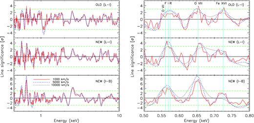
Gaussian line scan performed on the three XMM–Newton spectra shown in Fig. 3 using RGS between 0.45 and 2 keV and EPIC-pn from 2 to 10 keV. The results for three different line widths (FWHM) are shown. The line significance is calculated as square root of the ΔC-stat times the sign of the Gaussian normalization (positive/negative for emission/absorption lines). The right-hand panel is a zoom in the 0.5–0.8 keV energy range. The labels ‘F’, ‘I’, and ‘R’ refer to the forbidden, intercombination, and resonant lines of the O vii triplet, respectively.
3.2.1 Variability of the emission lines
We compare the observed fluxes of the strongest emission lines detected with the Gaussian scan for the three flux-resolved spectra in Fig. 6. Here, we use the results of the broad core (FWHM = 5000 km s−1), which maximizes the O vii and O viii significance. Owing to low statistics above 20 Å and the large line width, the O vii triplet is not well resolved. We therefore prefer to accumulate the fluxes of the O vii lines (resonance 21.6, intercombination 21.8, and forbidden 22.1 Å lines).
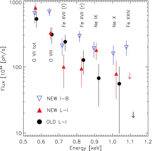
Fluxes of the strongest emission lines in the RGS stacked spectra of NGC 1313 X-1 (new intermediate–bright and low–intermediate and old low–intermediate). The fluxes of the O vii triplet have been accumulated. Notice the significant line variability especially in the new observations. The centroids of the lines have been slightly shifted for displaying purposes. In two cases only 90 per cent upper limits could be obtained.
It is clear that the emission lines significantly change, particularly during the bright state, but it is not straightforward to understand the variability of the emission measure distribution by simply comparing the single Gaussian lines (Fig. 6). However, the largest changes are seen in the O viii and other high-ionization lines, whose brightening might suggest a higher ionization state in the brighter spectrum. A self-consistent model is required to tie the results from multiple lines together and obtain further insights into the gas dynamics. This is done in Section 3.3.3 where we build-up photoionization and collisional-ionization emission models and perform model-scans on to the data.
The emission lines are broadly consistent with being at their rest wavelengths, although the centroids of the O vii and O viii lines in the bright state seem to be redshifted by ∼3000 km s−1 with respect to those of the low state as clearly shown in Fig. 7 for the O viii Lyman α line.
O viii Lyman α (1s–2p) velocity profile for the three RGS flux-resolved spectra of NGC 1313 X-1 (see also Fig. 3). A positive velocity indicates gas motion towards the observer. A line centroid of 18.967 Å (∼0.654 keV) is adopted (blue dashed line). The dotted vertical lines indicate shifts of |$\pm \, 3000$| km s−1. In the brighter state the line seems to exhibit a stronger red wing.
3.3 Photoionization modelling
An accurate photoionization model requires the knowledge of the radiation field. Pinto et al. (2020) have studied the thermal stability of ULX winds and compared them with other high Eddington sources such as narrow-line Seyfert 1 galaxies. In that paper, the SED of NGC 1313 X-1 was computed from IR to hard X-ray energies using literature data for the IR/optical/UV domain, complemented with the optical monitor aboard XMM–Newton. The X-ray spectral portion is provided by XMM–Newton and NuSTAR.
3.3.1 SED and stability curves
In this work, we construct the SEDs of the low-to-intermediate and intermediate-to-bright states using the low-energy portion (IR, optical, and far-UV) of the SED computed by Pinto et al. (2020) for the time-averaged spectrum of NGC 1313 X-1. For the high-energy part (soft and hard X-rays from 0.4 to 20 keV) we use the best-fitting continuum model, hot(mbb + mbb + comt), estimated in Section 3.1, Fig. 3 and Table 3. The absorption from the ISM is removed to obtain the intrinsic source spectrum. As shown in the spectral modelling, the SED above 10 keV is taken to be constant and is provided by the time-averaged NuSTAR spectrum. In fact, Walton et al. (2019) show that there is very little variability above 10 keV in the NuSTAR spectra of NGC 1313 X-1. The final SEDs are shown in Fig. 8 (top).
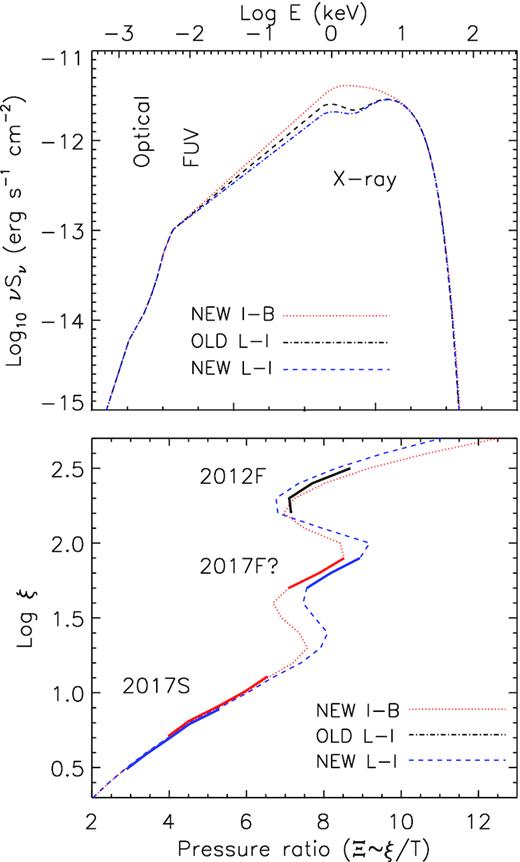
SED (top) and thermal stability curve (ionization parameter versus radiation/thermal pressure ratio, bottom) computed for the three spectra under investigation (see also Pinto et al. 2020). The solid lines in the bottom panel indicate the ionization parameters (±1σ errors) of the photoionized absorbers with higher significance in the archival (2012 at latest) and in the new (2017) spectra (see Table A1). The labels ‘F’ and ‘S’ refer to the fast and slow components, while ‘F?’ indicates the component with lower significance (≲3σ) in the new data.
The study of the relationship between the UV and X-ray flux will be done elsewhere, as well as a detailed time-resolved study of NGC 1313 X-1 comparing individual exposures or nearby pairs of exposures. For this work, we adopt a constant flux at the low energies (IR, optical, and far-UV). A study of some systematic effects introduced by the variability of the low-energy portion of the spectrum on to the ionization balance is briefly discussed in Pinto et al. (2020). They show that the main effect of a lower IR-to-UV flux is that of strengthening thermal instabilities in the plasma at intermediate temperatures and ionization parameters (e.g. Log T (K) ∼5 and Log |$\xi \, ({\rm erg\, s^{-1} \, cm}) \sim 1.5$|, respectively), but are not expected to produce major effects to our results.
The stability curves of the three spectra under investigation are very similar, which means that thermal instabilities should not affect the evolution of the wind. The study of thermal stability in each observation is relevant but is beyond the scope of this paper and will be done elsewhere.
We have tested the effect of non-Solar metallicity by calculating the ionization balance for Z between 0.5 and 1.5. Mildly sub-Solar (∼0.7) metallicities have very small effects on to the ionization balance with shifts comparable to those observed in Fig. 8. In particular, sub-Solar metallicities tend to increase the stable brunch. For Z ≳ 1.5 the unstable portion of the S curves increases. We therefore do not expect significant issues in our ionization balance calculation and spectral fits due to the uncertainties in the abundance pattern (see also Pinto et al. 2012).
3.3.2 Absorbing gas
Physical models are useful to determine the significance and nature of spectral features and to study plasma dynamics. We first focus on the modelling of the absorption features by using the fast xabs model in spex. xabs calculates the transmission of a slab of material, where all ionic column densities are linked through a photoionization model.
In principle, one could fit for several parameters of the xabs model such as the column density, NH, the ionization parameter, ξ, the line-of-sight velocity, vLOS, the velocity dispersion, the abundances, etc. However, in order to determine the best solution based on the observational data set, we perform automated spectral scans with the xabs model using a pre-defined multidimensional grid, similar to Kosec et al. (2018b). This technique is very efficient at locating possible solutions and prevents the fits from getting stuck in local minima, although is computationally expensive. It also provides a proxy for the absorption (emission) measure distribution if applied to line absorption (emission) models.
In this case, we construct a multidimensional grid of vLOS and ξ, whilst keeping free the NH. We adopted a vLOS blueshift ranging from 0 to 0.3c with steps of 500 km s−1 (comparable to the spectral resolution of the highest resolution instrument, RGS). A grid of log ξ from 0.1 to 5.0 with a 0.1 step is also used. We also do not fit the line widths but rather assume a grid of specific values similarly to the line scan in Section 3.2 (σv,1D = 1/2.355 FWHM of 500, 1000, and 5000 km s−1). All element abundances are chosen to be Solar for the same reasons mentioned in Section 3.3.1. Freeing the abundances could possibly provide significant improvements to the model search, but also increase the number of trials and the computing time. For every (ξ, vLOS, σv) combination a spectral fit is performed to each of the three flux-resolved spectra, starting from the baseline continuum model defined in Section 3.1, with the continuum parameters and the column density of the absorber free to vary, and the statistical fit improvement in |$\Delta \, C$| is recovered, as done for the Gaussian line scan in Section 3.2.
In Fig. 9, we show the probability distributions (in |$\Delta \, C$| and σ) from scans of the three spectra with σv = 500 km s−1 for the archival data and 1000 km s−1 for the two new spectra, which yield strong detections of both emission and absorption lines. As expected, our code finds and confirms the best-fitting ∼0.2c solution previously found in Pinto et al. (2016). Additional, weaker, peaks are found at lower ionization states (log ξ ∼ 0.6–0.8) and velocities (0.06–0.08c).
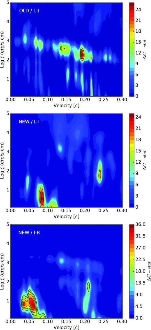
Photoionization absorption model scan of the archival data (top), the new low-to-intermediate (middle), and the new intermediate-to-bright spectra (bottom). The colour is coded according to the ΔC-stat fit improvement to the continuum model. The black contours refer to the 2.5 σ, 3.0 σ, 3.5 σ, and 4.0 σ confidence levels estimated through 3 × 10 000 Monte Carlo simulations.
As anticipated by the line scan in Fig. 5, the model scan shows that the absorber has radically changed, with the bulk of the absorption occurring at lower velocities (see Fig. 9) in the new data. These velocities agree with those suggested by PCA (see Section 4). Secondary peaks ranging from 0.2–0.25c with higher ξ similar to the archival data are also found in the new data albeit at much lower significance.
The two components with low or high (ξ, v) are likely independent as they account for different features in the RGS spectra. Although their individual significance is lower when both components (and the model for the line emission) are present in the model, they still provide substantial improvements to the fits (see Appendix A, Table A1 and Fig. A2).
We note that the global |$\Delta \, C$| levels are lower than those quoted in Pinto et al. (2016) because here we do not use the EPIC data below 2 keV, which has a larger count rate but lower spectral resolution than RGS, by more than an order of magnitude, in order to decrease the degeneracy. We have done a quick check by temporarily including pn data between 0.3 and 2 keV and obtained |$\Delta \, C$| of up to 48 with respect to the continuum (no absorption model) for the archival (OLD L–I) data and |$\Delta \, C$| up to 36 and 83 for the new spectra (NEW L–I and NEW I–B, respectively). These values correspond to the highest peaks shown in Fig. 9.
As can be seen in Fig. 9, our data selection is not optimal for plasmas with log ξ ≳ 4.0. The significance and thorough modelling of the putative, weaker, absorption features in the Fe K energy band (see Fig. 4) will require to combine data from EPIC and FPM-A/B as previously done in Walton et al. (2016a) and will be focus of a forthcoming paper.
3.3.3 Emitting gas
In order to determine the emission measure distribution of the plasma in the three spectra, we perform a similar model scan through the pion model in spex. The pion model calculates the transmission and emission of a photoionized plasma, whilst the xabs model is only optimized for absorption. The photoionization equilibrium in this model is calculated self-consistently. In principle, we could just use pion for both emission and absorption. However, this model re-calculates the ionization balance at every iteration and therefore is much more computationally expensive than the xabs model. For this reason, we prefer to use it only for emission studies. The pion model shares several parameters with xabs, but it also allows us to fit the density (for line emission) and retrieve more information on the plasma properties.
The emission lines detected with the Gaussian line scan are consistent with being at their rest-frame wavelengths (Fig. 6), which agrees with what was previously found in Pinto et al. (2016). We therefore build a simple grid of pion models with ξ between 0.1 and 5.0 with 0.1 steps and NH between 1020–24 cm−2. Based on the results of the line scan and the O vii triplet shape discussed in Section 3.2.1, we adopt the plasma density to be equal to nH = 1010 cm−3 and the line width σv = 1000 km s−1. We prefer not to increase the nH further as there are some issues with certain level populations at very high densities in pion. These ξ grids are used for the pion model, which is then an additive component in our spectral model on top of the continuum model (the xabs absorption component is removed from this model). For the pion model, we also adopt covering fraction equal to zero (i.e. using pion only to produce emission lines) and solid angle Ω = 4π. Fitting additional parameters such as Ω might provide even better fits but would significantly increase the computing time. Zero line-of-sight velocity is adopted here.
We run the model scan for the three spectra in investigation and plot the results in Fig. 10. Each panel shows the probability distribution of the emitting gas in terms of ΔC-stat and the confidence level expressed in σ, which is constrained using Monte Carlo simulations (i.e. including look-elsewhere effects). As we predicted above, the main peaks of the distributions show up at lower ionization parameters during the 2017 observations, particularly in the low-flux spectrum. However, the picture seems rather complex with evidence for multiphase structure and larger fractions of hotter gas during the high state.
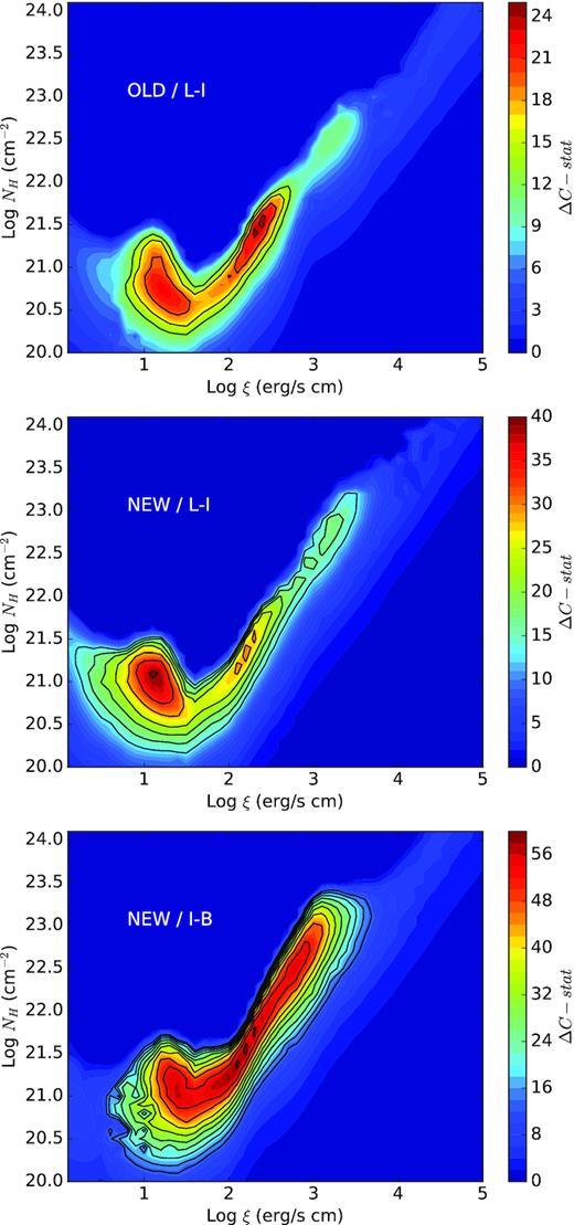
Photoionization emission model scan of the archival data (top), the new low-to-intermediate spectra (middle), and the new intermediate-to-bright spectra (bottom panel). The colour is coded according to the ΔC-stat fit improvement to the continuum model. The black contours refer to the 2.5σ, 3.0σ, 3.5σ, 4.0 σ, etc. confidence levels estimated through 10 000 Monte Carlo simulations for each spectrum. Negative values of ΔC-stat for high NH at low-to-mild ξ are kept to zero for displaying purposes.
4 PRINCIPAL COMPONENT ANALYSIS
In this section, we use an alternative technique to search for time-dependent spectral features at lower spectral resolution using PCA and the high-statistics EPIC-pn spectra to search for spectral features that respond to continuum variations.
In the field of active galactic nuclei, PCA has proven to be a reliable tool to detect broad-band or narrow spectral features that have correlated variability (see e.g. Mittaz, Penston & Snijders 1990; Francis & Wills 1999; Vaughan & Fabian 2004; Miller et al. 2007; Miller, Turner & Reeves 2008; Parker et al. 2014). For instance, Parker et al. (2017b) used PCA to detect the spectral component of the ultrafast (∼0.2c) outflow in narrow-line Seyfert 1 IRAS 13224−3809 thanks to the fact that the wind responds to the variations in the source continuum (Parker et al. 2017a; Pinto et al. 2018). They identified a series of variability peaks in both the first PCA component and Fvar spectrum, which correspond to the strongest predicted absorption lines from the ultrafast outflow previously found in high-resolution X-ray spectra. The main requirements for this method to be successful are (a) availability of a large data set, (b) source variability at time-scales larger than the time slices used (typically 1–10 ks), and (c) wind and continuum correlated variability.
We apply this technique, using the code of Parker et al. (2017a), to the whole NGC 1313 X-1 EPIC-pn data in order to search for similar peaks (all 12 observations in Table 1). We adopt 10 ks time bins and a logarithmic energy grid for a total of 165 pn spectra. The results for principal component one, PC1, are shown in Fig. 11. Some features appear at intermediate energies (1–3 keV) that would correspond to a 0.08c outflow if we identify them with the strongest transitions in this energy band (also detected in IRAS 13224–3809). At high energies noise dominates and it is difficult to obtain further information, while at low energies either PCA is not very sensitive to the features or they are weakly correlated to the continuum or the variability is weaker in the soft band. There is an interesting tentative drop at 5.9 keV similar to the bright spectrum (Fig. 5).
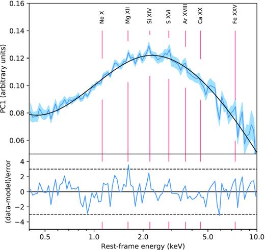
XMM/EPIC-pn PCA first-order spectrum, calculated from the entire data set (top). The main relevant transitions, blueshifted by 0.08c, are marked by vertical lines, and the shaded area shows the 1σ errors. The black line shows a spline fit to these data. The bottom panel shows the residuals to this fit, in units of standard deviations. Dashed horizontal lines mark the 3σ levels.
We fit the PCA spectrum with a cubic spline, using the univariateSpline function from scipy, weighting the points by the inverse of their errors. This gives a reasonable description of the broad-band shape, which we can then use to estimate the line significances. For the transitions that have clear corresponding peaks in the PCA spectrum (Ne x, Mg xii, Si xiv, S xvi, and Ar xviii), we calculate their deviation from the spline in σ (1.2, 3.6, 2.5, 1.7, and 0.8, respectively). We convert these to probabilities, assuming Gaussian statistics, and multiply them together to calculate the probability of finding five lines of this strength at the same blueshift. We then account for the number of trials by dividing by the number of resolution elements over the relevant range of velocities (for v = 0 to v = 0.4c, at 2 keV, this gives ∼8 resolution elements). This gives a final chance probability of 2.75 × 10⁻⁷, or 5.0σ. Considering only the strongest and most obvious three features (Mg xii, Si xiv, and S xvi) this falls to P = 2.8 × 10⁻⁶, or 4.5σ.
We attempt to repeat the PCA analysis using only the new data from the 2017 campaign and obtained consistent results albeit with higher noise. The archival data alone, where strong absorption was detected above 1 keV, is not ideally deep for our PCA analysis, but a quick check shows a weak peak above 1 keV, interestingly at the same location of the absorption features detected by the line scan (see Figs 3 and 5, and previously published in Pinto et al. 2016 for both RGS and EPIC spectra).
5 DISCUSSION
5.1 The NGC 1313 X-1 campaign
It is currently believed that the majority of ULXs consists of stellar-mass compact objects accreting above the Eddington limit by factors of a few up to hundreds, particularly after the discoveries of pulsars in some ULXs and mildly relativistic winds as predicted by models of super-Eddington accretion. This research field is rather young and several problems are still to be solved regarding the nature and launching mechanism(s) of the winds, their energy budget and effects on the circumstellar medium and on the life of the binary system.
We have been awarded 6 orbits targeting the NGC 1313 galaxy with XMM–Newton with the aim of achieving a better understanding of ULX winds. Some of these observations have been taken simultaneously with NuSTAR in order to improve the coverage of the hard X-ray band and Chandra to search for further narrow lines in the 2–7 keV energy band, which is not covered by RGS and where EPIC has low-energy resolution. In this first paper, we focus on the study of the wind in NGC 1313 X-1 and, in particular, its variability with the ULX spectral state based on the well-known spectral variability (Middleton et al. 2015a) and detection of emission and absorption lines (Pinto et al. 2016). We notice that this campaign has already provided interesting results such as the first discovery of pulsations in NGC 1313 ULX-2 (Sathyaprakash et al. 2019), which added a new candidate to the presently small list of PULXs.
The study of the broad-band spectral continuum is presented in a companion paper (Walton et al. 2019). The search for additional narrow spectral features at intermediate energies (1–7 keV) with Chandra is presented in Nowak et al. (in preparation). The spectral-timing analysis and the application of Fourier techniques on to our new data are also described in another paper of this series (Kara et al. 2020) where we show the first discovery of a soft lag in NGC 1313 X-1 similarly to other two ULXs with wind detections: NGC 5408 X-1 and NGC 55 X-1.
Here, we briefly note that our observations scheduled in pairs separated by long periods of 2–3 months enabled us to detect NGC 1313 X-1 at different fluxes covering a smooth range of spectra (see Swift/XRT light curve in Fig. 2 and spectra Figs 3 and A1). The source shows a continuum behaviour typical of the subclass of ULXs with hard spectra at low fluxes and softer, broad disc-like, spectra at high fluxes in according to the classification of Sutton et al. (2013).
XMM–Newton EPIC and RGS spectra from observations with similar flux levels and spectral shape have been combined to compare the wind appearance in three different epochs and luminosity regimes (see Fig. 3). The three broad-band spectra have been modelled with a multicomponent spectral continuum model consisting of two modified-disc-blackbody components to reproduce the classical two broad peaks around 1 and 3–7 keV in the low state (see Table 3, Figs 3 and A1) plus a comptonization component to fit the hard tail often found in ULXs (see e.g. Walton et al. 2018).
Our results are broadly consistent with those presented in the paper by Walton et al. (2019) to whom we refer for a more detailed analysis of the X-ray broad-band continuum and of its variability. During the bright state the spectral curvature around 2 keV decreases (see Fig. 3) and the two thermal components are not well distinguished in our model (see Table 3) but this has no effects on the search for narrow spectral features.
5.2 The wind
5.2.1 Emission lines
Strong positive residuals are found in correspondence of the transition energies of several ions such as O vii, O viii, Ne x, and Fe xvii in agreement with Pinto et al. (2016) and confirmed in this work (see Figs 4 and 5).
Some emission lines clearly change, becoming stronger in the softer, bright, state (see Fig. 6). This occurs for O viii and several lines around 1 keV. However, their equivalent widths are lower in the bright state because the continuum around 1 keV is about four times higher than in the L–I hard state. This broadly agrees with the results Middleton et al. (2015b) who showed that the residuals around 1 keV weaken in the bright spectra. Hints of variability in both the absorption and emission lines were already found in Pinto et al. (2016), but this is the first time that we can robustly confirm it. Photoionization emission modelling further strengthens the variability of the emission lines with the spectral state and with the time (see Fig. 10). This is the first unambiguous evidence that the emission lines are intrinsic to the ULX.
The emission lines are stronger, broader, and likely redshifted in the bright state (see Fig. 7), which would be consistent with them being emitted from the outer disc and progressively stronger at high accretion rates. They resemble the flat-top profile with steep wings of Paschen lines in broad-line regions of AGN or disc winds of X-ray binaries such as GRO J1655−40 (Soria, Wu & Hunstead 2000). In this case, the emission lines may be produced near or outside the spherization radius, in the irradiated part of the disc, with their strength proportional to accretion rate (see cartoon in Fig. 12).
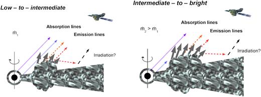
Simplified scheme of a variable high mass accretion rate source. The compact object is surrounded by an inner corona (or accretion column) and a thick disc of matter from the companion star. Left-hand panel: Above the Eddington limit (|$\dot{m}_1 \gt \dot{m}_E$|) radiation pressure thickens the disc and launches a powerful wind from a region around the spherization radius (|$R\sim 25\, R_\mathrm{ S}$| for vesc ∼ 0.2c). Right-hand panel: At even higher accretion rates (|$\dot{m}_2 \gt \dot{m}_1 \gt \dot{m}_E$|), the source simultaneously brightens and softens, the spherization radius extends to larger radii and a cooler phase of the wind is launched at larger radii (|$\sim 150\, R_\mathrm{ S}$| for 0.08c). The emission lines, presumably coming from the outer irradiated disc, also become stronger and broader. These trends are observed in NGC 1313 X-1.
The g, r line ratios of the O vii triplet suggest a high-density hybrid gas (nH ∼ 1010–12 cm−3) where both recombination and collisional processes occur (Porquet & Dubau 2000). Models of collisionally ionized emitting plasma provide similar results to those obtained using photoionization equilibrium, but generally slightly worse fits (see Appendix A and Fig. A3). Photoionization is therefore preferred, but we cannot rule out some contribution from collisions e.g. due to shock between the wind and the companion star or the surrounding interstellar medium.
The luminosity of the line-emission component is remarkably high (|$L_{\, 0.3-10\, \rm keV}\gt 10^{38}$| erg s−1), about 2–3 orders of magnitude higher than winds – including colliding winds – in classical supergiant X-ray binaries (hosting a neutron star accreting below the Eddington limit from a supergiant OB star, see e.g. El Mellah & Casse 2017) and much higher than lines from accretion disc coronae of low-mass X-ray binaries (LMXBs; see e.g. Kallman et al. 2003). CCD spectra provide comparable results (see e.g. Middleton et al. 2015b and references therein). Such luminosity is consistent with that measured by Wang et al. (2019) for the plasma producing blueshifted emission lines in Chandra and XMM–Newton spectra of a transient ULX in NGC 6946.
Interestingly, both the column densities of 1021–22 cm−2 and the volume densities (nH ∼ 1010–12 cm−3) measured for the line-emitting gas in NGC 1313 X-1 (assuming Solar abundances, see Table A1) are comparable to those measured in accretion disc coronae of some LMXBs (see e.g. Cottam et al. 2001; van Peet et al. 2009; Iaria et al. 2013; Psaradaki et al. 2018). We note that we adopt a full solid angle for the emitting gas in order to speed up our fit in this paper. A lower solid angle of e.g. Ω/4π ∼ 0.1, as found in the plasmas around many X-ray binaries, would yield a larger column density in NGC 1313 X-1. We remark that our volume density estimates might be affected by uncertainties due to the low statistics above 20 Å and the possible contribution from collisional ionization. For a volume density nH ∼ 1012 cm−3 and an ionization parameter ξ ∼ 100 erg s−1 cm, using equation (3), we obtain a distance R ∼ 0.5 U.A., which is comparable to the size of the Roche lobe estimated for the pulsating ULX NGC 7793 P13 by Fürst et al. (2018).
5.2.2 Absorption lines
In Pinto et al. (2016), a highly significant ultrafast outflow was detected in NGC 1313 X-1 through the combination of the EPIC and RGS absorption features in the soft X-ray band. Here, we confirm the detection, even using only RGS below 2 keV (albeit at lower significance because of the more restrictive data selection used in this work; see Fig. 5, top left panel). The wind has remarkably changed from 2012 (and before) to 2017 with the fast, ∼0.2c, and highly ionized, log ξ ∼ 2.3, component significantly weaker and a slower, 0.08c, and lower ionization, log ξ ∼ 0.8, phase now also clearly detected (see Fig. 9). The relative strengthening of such a ‘cooler’ phase compared to the ‘hotter’ one is more evident in the bright state. The absorption lines of this new cooler phase appear broader (see Fig. 5 and Table A1).
These findings are corroborated by the results of the PCA (see Fig. 11) which showed new features at intermediate energies that agree with the most relevant Lyman α lines of Mg, Si, S, and Ar all blueshifted by about 0.08c. The variations in the wind velocity and ionization parameter may explain why its features are weak in the PCA. This technique commonly shows stronger features in coherently changing winds and at consistent velocities.
5.3 A scenario of variability in the accretion rate
Our results are consistent with a scenario in which a higher accretion rate has occurred during the middle and the end of 2017 and, possibly, during the previous year (as suggested by the high variability and average flux levels in the Swift light curve from 2016, see Fig. 2). We speculate that the recent higher accretion rate has caused the brighter and softer state of the source, the appearance of a cooler and slower component of the wind, the strengthening of the emission lines, and the broadening of most emission and absorption lines.
Regarding the emission lines, assuming that they are produced near the spherization radius, an increase in the accretion rate would move the spherization radius outwards, broadening the emitting region and the velocity pattern. Otherwise, if they are emitted from the portion of the disc external to the spherization radius, then their broadening might be caused by the inner wind that increasingly shields the outer disc at higher |$\dot{m}$|, which lowers the ionization of the disc and enables emission of (broader) lines from smaller radii, where previously the ions were fully ionized.
Assuming that the velocities measured in our line of sight are proxies for the (escape) launching velocities of the wind, we estimate an outer launching radius (|$\sim 150\, R_\mathrm{ S}$| for 0.08c) than for the faster component detected previously (|$\sim 25\, R_\mathrm{ S}$| for 0.2c). The smaller launching radius and the higher velocity are comparable to those estimated in the inner regions of the disc through GR-MHD simulations, while the slower and outer wind are similar to the outer region where the wind becomes clumpy (see e.g. Takeuchi et al. 2013; Kobayashi et al. 2018).
The emission lines would be produced even further out (see Fig. 12). During the L–I state in 2017 September the imbalance between the slow and fast phases seems milder than in the I–B state (see Fig. 9 and Table A1), maybe due to a lower accretion rate. The fast wind could be still hard to detect if the inner regions are obscured by the newly discovered cooler phase of the wind (as illustrated in Fig. 12, right-hand panel). We note that the lower statistics of the new L–I state prevent us from making strong claims. Finally, the kinetic power of the two main wind components is comparable (|$L_{\rm kin, \, Fast / Slow} \sim 1$|). This is because the velocity of the fast component |$v_{\rm \, Fast} \sim 2\!-\!3 \, v_{\rm \, Slow}$|, the ionization parameter |$\xi _{\rm \, Fast} \sim 10\!-\!30 \, \xi _{\rm \, Slow}$|, the ionizing luminosity (see Table A1) |$L_{\rm ion, \, I-B} \sim 1.5 \, L_{\rm ion, \, L-I}$| (see e.g. Table 3), and the kinetic power goes as |$L_{\rm kin} \propto L_{\rm ion}\, (v^3_{\rm out} / \xi)\, C_V\, \Omega$|. Here, we assume the same covering factor and opening angle of the wind components, which can of course differ.
In summary, the general picture may be that the X-ray continuum comes from the inner (supercritical) disc, the line absorption comes from the wind launched inside the spherization radius and the line emission comes from the thinner, slower wind launched from the irradiated standard-disc surface outside the spherization radius. This is consistent with the fact that blueshifted emission lines are seen in NGC 55 ULX (see Pinto et al. 2017), a spectral hybrid between soft ULXs and supersoft ultraluminous sources (see e.g. Feng et al. 2016) that is believed to be viewed at a larger inclination than NGC 1313 X-1. Further, in-depth, work is required to confirm this scenario and indeed several forthcoming papers are being produced focusing on the broad-band variability spectral variability on different time-scales (e.g. Walton et al. 2019; Kara et al. 2020).
5.4 Future studies of ULX winds with ATHENA
Current X-ray observatories such as XMM–Newton and Chandra have opened up new research channels to understand ULXs and, more in general, super-Eddington accretion. However, their high-energy-resolution spectrometers have low effective area, requiring exposure times of 1–2 d to achieve high statistics. This prevent us from tracking the wind variability down to time-scales as short as 1 ks (or even less), which are similar to the time lags found in some ULXs including NGC 1313 X-1 (Kara et al. 2020) and those shown by the PCA (Section 4). The study of the winds behaviour at such time-scales could place stronger constraints on their nature and structure. The future X-ray mission XRISM (Guainazzi & Tashiro 2018) will enable to detect and resolve features from hotter wind phases in the hard X-ray band (∼2–10 keV), providing complementary information to RGS but still requiring days of observations (see Pinto et al. 2020 for a XRISM simulation of NGC 1313 X-1).
X-ray astronomy will dramatically change in the 2030s after the launch of ATHENA (Nandra et al. 2013). Its X-ray Integral Field Unit (X-IFU), in particular, will be the first X-ray microcalorimeter to provide both high spatial (5 arcsec) and spectral (2.5 eV) resolution with an effective area an order of magnitude higher than any current high-spectral-resolution X-ray detector, which gives an improvement of almost 2 orders of magnitude in the detection of narrow features in the canonical 0.3–10 keV X-ray energy band (see e.g. Barret et al. 2018).
We simulate three X-IFU spectra of NGC 1313 X-1 using the best-fitting wind models of the three RGS spectra (see Table A1 and Fig. A2) and adopting an X-IFU exposure time of 25 ks each. The expected results are extremely promising with the lines obviously changing between the states, while in RGS spectra – without a careful analysis – might appear comparable (Fig. 13). A short snapshot of 1 ks with the X-IFU will still provide a high signal-to-noise spectrum with several emission and absorption lines detected at |$5\, \sigma$| each. This will enable to study the wind at the variability time-scales probed by the PCA (Section 4) and by ULX soft lags (few 10-to-1000 s). Moreover, the X-IFU will detect winds in ULXs at much larger distance, boosting the explored volume of ULXs and determining wind properties at much higher accuracy. The comparison between their properties with those of the interstellar cavities around many ULXs will determine the role ULXs feedback, particularly in the early Universe.
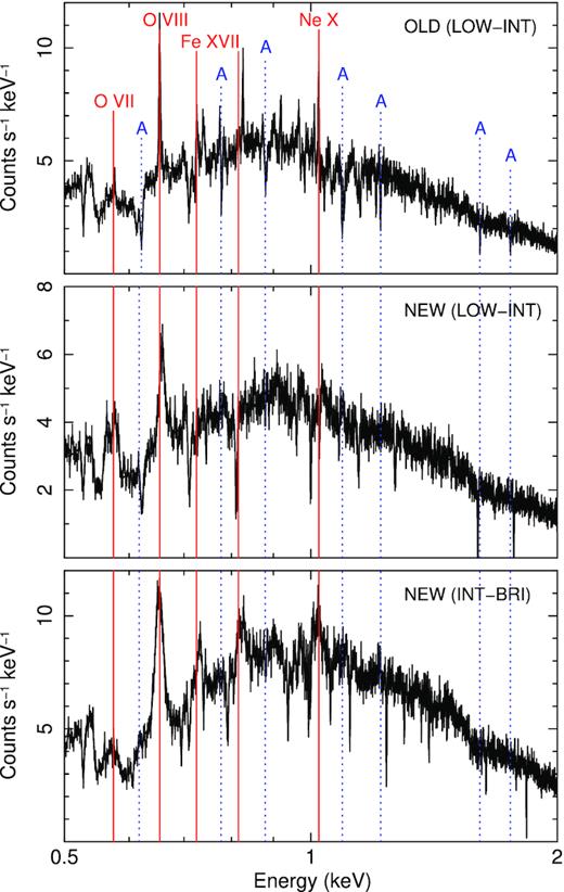
ATHENA / X-IFU simulations of the ULX NGC 1313 X-1 for the three spectra with overlaid the best-fitting multiphase wind model. The wind model consists of photoionized emitting plasma and a two-phase absorber (see Table A1 and Fig. A2). Cosmic X-ray background and particle background are accounted for. The X-IFU response matrix is dated 10-2018 with 1.4 m2 effective area at 1 keV. Note how the lines strongly differ in these spectra.
6 CONCLUSIONS
Most ULXs are believed to be powered by super-Eddington accreting neutron stars and black holes. If the compact object is not a neutron star with a magnetar-like magnetic field, the disc is expected to thicken and launch powerful winds through radiation pressure or magnetic fields might launch winds themselves. Evidence of winds has been found in the ULXs through the high-resolution spectrometers onboard XMM–Newton. In order to understand the wind geometry, its relationship with the accretion rate and the source state, we undertook a large observing campaign with XMM–Newton to study the NGC 1313 (UL)X-1, which exhibits strong rest-frame emission and blueshifted absorption lines.
The new observations show remarkable wind variability, with the previously known fast component (∼0.2c) to have weakened, and a new, cooler and slower (∼0.08c), wind component appearing. Significant variability is found in the highly significant emission lines, showing for the first time that they are most likely produced in the accretion disc or the outer wind. We describe the simultaneous change of the wind and the spectral continuum in terms of variability in the super-Eddington accretion rate. The geometry that can describe the observables and agrees with the theoretical models of super-Eddington accretion discs, implies that the continuum is emitted within the inner supercritical regions, the line absorption is produced by the wind launched near the spherization radius and the emission lines come from a slower wind component in the outer, likely irradiated, disc.
ACKNOWLEDGEMENTS
This work is based on observations obtained with XMM–Newton, an ESA science mission funded by ESA Member States and USA (NASA). CP, MP, and FF are supported by European Space Agency (ESA) Research Fellowships. We acknowledge support from STFC and ERC Advanced Grant Feedback 340442 and the European Union’s Horizon 2020 Programme under the AHEAD AO5 project (grant agreement n. 654215). We also thank J. de Plaa and M. Mehdipour for support in optimizing spex and I. Psaradaki for help with PYTHON. We thank the XMM–Newton SOC and, in particular, Jan-Uwe Ness for excellent support in optimizing our observing campaign. We finally acknowledge the anonymous referee for useful comments that improved the clarity of the paper.
Footnotes
REFERENCES
APPENDIX A: TECHNICAL DETAILS
In this section, we put the plots and tables that are excluded from the main body of the paper to facilitate the reading.
Fig. A1 (left-hand panel) shows the EPIC-pn spectra extracted for the 12 individual exposures. In the right-hand panel the spectra are in the same units, but have been shifted in the Y-axis, multiplying for a constant for display purposes.
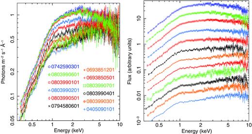
Left-hand panel: XMM–Newton/EPIC-pn spectra for both archival and new (080399) observations. The spectra cover a continuous distribution of fluxes from low (ultraluminous-hard) to the bright (broadened-disc) states. Most flux variations occur in the soft-intermediate X-ray energy band, while the spectra overlap beyond 5 keV. Right-hand panel: same data and colour code as shown in the left-hand panel, but here the spectra have been shifted along the Y-axis for displaying purposes.
The best-fitting wind models with the three main emission and absorption components are shown in Fig. A2 with their relevant parameters detailed in Table A1. We also quote the spectral fit improvement ΔC and the significance σ for all the components. We report them in the case where each component was fit alone with the continuum as for the model scans (ΔCa and σa) and also where all emission and absorption components where included in the model (ΔCe and σe). The latter represents a test for independence among the several components. Here their individual significances decrease but each of them still provides substantial improvements to the spectral fits, some of which well beyond 3σ and 4σ.
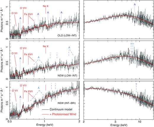
RGS (left), EPIC-pn, and FPM A,B(right) spectra with overlaid the best-fitting multiphase wind model (red line) and the broad-band continuum model (black line). The wind model consists of a two-phase photoionized absorber and a photoionized emission component (see Table A1). Data and line labels are the same as in Fig. 3.
NGC 1313 X-1: main wind components.
| Phase | Parameter | OLD L–I | NEW L–I | NEW I–B |
|---|---|---|---|---|
| EMI | NH | 3.0 ± 0.8 | 1.4 ± 0.3 | 3.5 ± 1.3 |
| (rest) | log ξ | 2.4 ± 0.1 | 1.1 ± 0.1 | 2.2 ± 0.2 |
| vLOS (km s−1) | 100 ± 300 | 2000 ± 700 | −550 ± 350 | |
| vσ (km s−1) | 200 ± 200 | 1600 ± 400 | 2100 ± 500 | |
| ΔCa(e) | 25(21) | 40(35) | 55(50) | |
| σa(e) | 3.5(3.1) | >4(>4) | >4(>4) | |
| ABS 1 | NH | 0.3 ± 0.1 | 0.4 ± 0.1 | 0.7 ± 0.1 |
| (slow) | log ξ | 0.8 ± 0.3 | 0.7 ± 0.2 | 0.9 ± 0.2 |
| vLOS (c) | 0.081 ± 0.004 | 0.084 ± 0.003 | 0.084 ± 0.004 | |
| vσ (km s−1) | 700 ± 400 | 800 ± 400 | 3500 ± 1500 | |
| ΔCa(e) | 17(10) | 25(21) | 38(30) | |
| σa(e) | 2.6(2.0) | 3.5(3.2) | >4(> 4) | |
| ABS 2 | NH | 4.1 ± 1.5 | 0.7 ± 0.2 | 0.6 ± 0.2 |
| (fast) | log ξ | 2.3 ± 0.1 | 1.8 ± 0.1 | 1.8 ± 0.1 |
| vLOS (c) | 0.191 ± 0.002 | 0.240 ± 0.002 | 0.210 ± 0.002 | |
| vσ (km s−1) | 100 ± 100 | 420 ± 260 | 120 ± 120 | |
| ΔCa(e) | 26(21) | 18(15) | 19(13) | |
| σa(e) | 3.7(3.1) | 2.9(2.5) | 2.9(2.3) |
Notes. Best-fitting wind components: photoionized emission (EMI) and absorption (ABS, see also Figs 9 and 10). The ionization parameters are in log (ξ, erg cm s−1) and the column densities, NH, in 1021 cm−2. The line-of-sight velocities, vLOS, are in units of light speed c for ABS 1,2 and km s−1 for EMI (assumed positive for blueshift and motion towards the observed); the line widths, vσ, are in km s−1. The spectra are defined in Section 2.4.2. The ΔCa(e) refer to the ΔC-statistics of each component computed when the component is the only one in model (a) or when the other two are included (e). The same applies to the detection significances, σa(e), which are evaluated with Monte Carlo simulations.
In Fig. A3, we show the search for a shocked wind performed by scanning an emission model of gas in collisional equilibrium (cie model in spex) over the three flux-/time-resolved spectra: archival low-to-intermediate state (solid black line), the new low-to-intermediate state (dashed green line), and the new intermediate-to-bright state (dotted red line); see also Section 3.3.3. For a comparison with a similar scan using photoionization emission models see Fig. 10. Collisional ionization equilibrium provides generally worse fits than photoionization except for the archival data.
![Wind search through scans of collisional ionization emission models for the archival low-to-intermediate (solid black line), the new low-to-intermediate (dashed green line), and the new intermediate-to-bright spectra (dotted red line); see also Section 3.3.3. The X-axis shows the plasma temperature, kT (slightly shifted for displaying purposes). The top panel shows ΔC-stat fit improvement for each kT and the bottom panel is the corresponding emission measure [Log $n_\mathrm{ e} n_{\rm H} V \, ( 10^{58}$ cm−3)].](https://oup.silverchair-cdn.com/oup/backfile/Content_public/Journal/mnras/492/4/10.1093_mnras_staa118/1/m_staa118figa3.jpeg?Expires=1750675721&Signature=tT06ra2RUjFgxI9Uf5EOYWHiclAoALkjJVaw5ntJ8GA0p5~l92lI~ye6iIh0yt3nsSfkb7B0OzYt6wAmFGw0rI2bOveJCePoBegAPEXUDBGraL-72YY6bz5E~AKoGXZPEQiF5MlQAPK3D1kAsd72c9Yhx6ZexkqaME4JRdrq9qqpHjUlZm7uwFPRheRKNPXCWBIJiwrEJwqIa8nz-lLaSIVjrZK7f8-CGELKtZqnItrGNhimSuPXT48--MxWt7Zr4lTHygdF9qaXWnz10-tLUURgIPxLiSqUHpXzOaQyO7gI30-UhDn1z8R28XKGutekrj1YVir5mKPlHGRUUsOmHA__&Key-Pair-Id=APKAIE5G5CRDK6RD3PGA)
Wind search through scans of collisional ionization emission models for the archival low-to-intermediate (solid black line), the new low-to-intermediate (dashed green line), and the new intermediate-to-bright spectra (dotted red line); see also Section 3.3.3. The X-axis shows the plasma temperature, kT (slightly shifted for displaying purposes). The top panel shows ΔC-stat fit improvement for each kT and the bottom panel is the corresponding emission measure [Log |$n_\mathrm{ e} n_{\rm H} V \, ( 10^{58}$| cm−3)].
