Population synthesis of exocometary gas around A stars

Marino, S; Flock, M; Henning, Th; Kral, Q; Matrà, L; Wyatt, M C

doi:10.1093/mnras/stz3487

ABSTRACT

The presence of CO gas around 10–50 Myr old A stars with debris discs has sparked debate on whether the gas is primordial or secondary. Since secondary gas released from planetesimals is poor in H₂, it was thought that CO would quickly photodissociate never reaching the high levels observed around the majority of A stars with bright debris discs. Kral et al. showed that neutral carbon produced by CO photodissociation can effectively shield CO and potentially explain the high CO masses around 9 A stars with bright debris discs. Here, we present a new model that simulates the gas viscous evolution, accounting for carbon shielding and how the gas release rate decreases with time as the planetesimal disc loses mass. We find that the present gas mass in a system is highly dependant on its evolutionary path. Since gas is lost on long time-scales, it can retain a memory of the initial disc mass. Moreover, we find that gas levels can be out of equilibrium and quickly evolving from a shielded on to an unshielded state. With this model, we build the first population synthesis of gas around A stars, which we use to constrain the disc viscosity. We find a good match with a high viscosity (α ∼ 0.1), indicating that gas is lost on time-scales ∼1–10 Myr. Moreover, our model also shows that high CO masses are not expected around FGK stars since their planetesimal discs are born with lower masses, explaining why shielded discs are only found around A stars. Finally, we hypothesize that the observed carbon cavities could be due to radiation pressure or accreting planets.

methods: numerical, circumstellar matter, planetary systems, accretion, accretion discs

1 INTRODUCTION

The discovery of circumstellar gas around young main-sequence stars with debris discs dates back more than two decades, with a few systems showing molecular emission at millimetre wavelengths (e.g. Zuckerman, Forveille & Kastner 1995) and others atomic absorption in the UV (Slettebak 1975), some of which varies with time (Ferlet, Vidal-Madjar & Hobbs 1987). Thanks to Herschel, it also became possible to study the gas component in the far-IR through atomic emission from ionized carbon and neutral oxygen (e.g. Riviere-Marichalar et al. 2012; Roberge et al. 2013; Cataldi et al. 2014), adding a third tool for the observational study of gas in systems with debris discs. Today, we know of about 20 systems with debris discs and gas detected in emission, and another ∼11 systems (with and without infrared excess) with circumstellar gas detected in absorption only (e.g. Montgomery & Welsh 2012; Iglesias et al. 2018; Rebollido et al. 2018; Welsh & Montgomery 2018).

While there has been some consensus on the origin of the absorption lines as arising from falling evaporating bodies (FEBs; Ferlet et al. 1987; Beust et al. 1990; Beust & Morbidelli 1996; Kiefer et al. 2014), no model has been completely successful at explaining the colder emitting gas at tens of au that is now found around ∼20 systems (e.g. Moór et al. 2011, 2015, 2017; Dent et al. 2014; Greaves et al. 2016; Lieman-Sifry et al. 2016; Marino et al. 2016, 2017; Matrà et al. 2017b, 2019), mostly through CO detections. Since CO molecules exposed to stellar and interstellar UV radiation will photodissociate in short time-scales (≲120 yr, Hudson 1971; van Dishoeck & Black 1988; Visser, van Dishoeck & Black 2009), the CO detected in some of these systems suggests that we are observing these systems at a very particular moment (e.g. at the later stages of protoplanetary disc dispersal, hereafter primordial origin) or CO and other gas species are being replenished in these systems (hereafter secondary origin). Zuckerman & Song (2012) proposed that gas could be released in the same collisional cascade that replenishes the dust levels in debris discs. The amount of gas and dust could then be used to infer the volatile composition of planetesimals. This scenario would be consistent with systems with the low CO levels observed, for example, around β Pic, HD 181327 and Fomalhaut. However, a significant fraction of the systems with detected CO would require planetesimals much richer in CO and/or CO₂ compared to Solar system comets, or gas release rates that are decoupled from the inferred dust production rates (Kral et al. 2017). Furthermore, the systems with the highest CO content have ages between 10–50 Myr and their content is not necessarily correlated with their debris disc-like dust (Moór et al. 2017). Therefore, these have been tagged as hybrid discs meaning they have primordial gas leftovers and secondary dust (Kóspál et al. 2013), although it is not clear how primordial gas has survived for so long in those systems.

A potential pathway to alleviate these tensions in the secondary origin scenario, is that the CO becomes shielded from UV radiation in systems with high gas content and its lifetime is much longer than in the unshielded case. While debris discs are optically thin hence dust cannot effectively shield the gas, CO can become self-shielded or shielded by molecular hydrogen (van Dishoeck & Black 1988; Visser et al. 2009). This is difficult since H₂ is unlikely to be present at high densities in this secondary origin scenario, and CO would need to be released at a very high rate to reach the necessary column densities to become self-shielded (Kral et al. 2017). However, carbon that is produced through CO photodissociation can also shield CO from UV photons, becoming ionized (Rollins & Rawlings 2012). Carbon and oxygen are expected to viscously evolve and form an atomic accretion disc (Kral et al. 2016), even if the stellar luminosity is high enough to blow out carbon since it can remain bound due to self-shielding and interactions with more bound species such as oxygen (Fernández, Brandeker & Wu 2006; Kral et al. 2017). Kral et al. (2019) found that if viscosities were low or the CO input rate high, enough carbon could accumulate to shield CO and explain hybrid discs as shielded discs of secondary origin.

So far, none of the above studies has considered the viscous evolution of an exocometary gas disc coupled with the time-dependent gas release rate. If the release of gas is regulated by the mass-loss rate in the planetesimal disc, then we expect this to decrease steeply with time relaxing into a collisional equilibrium (e.g. Dominik & Decin 2003; Krivov, Löhne & Sremčević 2006; Wyatt et al. 2007a). This means that the total gas mass input into a system depends strongly on its previous evolution if the gas lifetime is similar or longer than the age of the system (or collisional time-scales). If viscosities are low, this could well be the case for shielded discs, thus collisional evolution cannot be neglected a priori. In this paper, we consider the effect of an evolving mass input rate on the viscous evolution of the gas in the system, particularly we focus on CO and carbon. This paper is structured as follows. We first present our model and numerical simulations in Section 2. Then in Section 3, we use this model to produce a population synthesis of A stars with debris discs that release gas, which we compare with observations. In Section 4, we show that the same model applied to FGK stars is also consistent with observations. In Section 5, we discuss our results and some of our assumptions, and finally in Section 6, we report our conclusions.

2 MODEL

The gas evolution is treated with a simple viscous evolution 1D model, focusing only on the radial dimension and assuming axisymmetry (similar to Moór et al. 2019). In this model, gas is input into the system at the radial locations of the planetesimal belt, from where it is allowed to viscously evolve. The gas surface density evolution, Σ_G, is then set by the usual viscous evolution equation (Lynden-Bell & Pringle 1974) with the addition of an input source that arises from a collisional cascade of planetesimals, |$\dot{\Sigma }^{+}_\mathrm{coll}(r,t)$|⁠,

$$\begin{eqnarray*} \frac{\partial \Sigma _{\rm G}}{\partial t} = \frac{3}{r} \frac{\partial }{\partial r} \left[r^{1/2} \frac{\partial }{\partial r} (\nu \Sigma _{\rm G}r^{1/2}) \right] + \dot{\Sigma }^{+}_\mathrm{coll}(r,t), \end{eqnarray*}$$

(1)

where ν is the kinematic viscosity. In equation (1), we have also made the usual approximation that the orbital velocity does not significantly differ from circular Keplerian rotation.

Rather than studying Σ_G, in this paper we are mainly interested in following the evolution of CO, C, and O, which can have significantly different distributions (Kral et al. 2016). Therefore, instead of solving equation (1), we solve for the evolution of the surface density of each gas species Σ_i by advecting its mass at the viscous radial velocity, v_r, hence

$$\begin{eqnarray*} \frac{\partial \Sigma _i}{\partial t} &=& - \frac{1}{r}\frac{\partial }{\partial r} (r v_r \Sigma _i) + \dot{\Sigma }_i^{\pm }(r,t), \\ \Sigma _{\rm G}v_r &=& - \frac{3}{\sqrt{r}} \frac{\partial }{\partial r} (\nu \Sigma _{\rm G}\sqrt{r}), \\ \Sigma _{\rm G}&=& \sum _{i} \Sigma _i , \end{eqnarray*}$$

(2),(3),(4)

where |$\dot{\Sigma }_i^{\pm }(r,t)$| represents the additional production and destruction processes (e.g. CO photodissociation, see below) and v_r the radial velocity of the gas. Equation (2) is a continuity equation with a source term, while equation (3) is the conservation of angular momentum which is applicable to the total mass. We solve equations (2) and (3) using first-order explicit finite-volume update following Bath & Pringle (1981) and Booth et al. (2017). We also include the diffusion of the gas species, that is given by

$$\begin{eqnarray*} \frac{\partial f_i}{\partial t} = \frac{1}{r\Sigma _{\rm G}} \left(r \nu \Sigma _{\rm G}\frac{\partial f_i}{\partial r}\right), \end{eqnarray*}$$

(5)

where f_i = Σ_i/Σ_G and we have taken a Schmidt number of unity (Stevenson 1990; Turner et al. 2006). The addition of equation (5) accounts for the diffusion due to turbulent mixing rather than an accretion flow. It does not affect the total surface density, but the relative abundances of CO, carbon, and oxygen.

For the viscosity, we make the standard assumption of an alpha disc model, with |$\nu =\alpha c_\mathrm{ s}^2/\Omega _\mathrm{K}$|⁠, where c_s is the sound speed and Ω_K the Keplerian speed. The sound speed is calculated from the gas temperature, which is fixed and taken equal to the blackbody temperature for simplicity (⁠|$T=278 L_\star ^{1/4} r^{-1/2}$|⁠) and a mean-molecular weight that can vary between 28 and 14 depending on if the gas is dominated by CO or by atomic oxygen and carbon. This choice of parametrization of ν is arbitrary, but it offers a form simple enough to understand the gas evolution. Note that we expect α to be smaller than unity, although its value has only been constrained between 10⁻⁴ and 0.5 (Kral et al. 2016, 2019; Kral & Latter 2016; Moór et al. 2019).

The input of gas in the system happens through the release of volatile species that escape after the breakup of volatile rich bodies in a collisional cascade. This release is spatially confined to a planetesimal belt that extends in radius and is radially resolved by our simulations. Furthermore, we assume that the released gas is completely dominated by CO. In principle, other molecular species such as CO₂, H₂O, HCN, etc. could also be released; however, current observations are roughly consistent with CO dominated gas release. The addition of other gas species is discussed in Section 5.1.1.

Once CO is released and exposed to interstellar UV radiation it will photodissociate into carbon and oxygen on a short time-scale of 120 yr (Visser et al. 2009), or even shorter depending on the strength of the stellar UV flux (Matrà et al. 2017a). For example, a stellar luminosity higher than 20 L_⊙ will shorten the CO photodissociation time-scale to less than 10 yr within ∼100 au if unshielded (see fig. 1 in Kral et al. 2017). This time-scale, however, can be much longer if the CO column densities are high enough to shield itself or if neutral carbon is present. The latter is of special interest since depending on how fast CO is released and carbon viscously spreads, it could explain the existence of large amounts of CO in 10–50 Myr old systems (Kral et al. 2019).

In this work, we will focus solely on the effect of interstellar UV radiation and will neglect the stellar contribution. This is justified by the two following reasons. First, most of the discs that we want to explain have stellar luminosities below 20 L_⊙ and debris disc sizes of ∼100 au, which means that if CO was completely unshielded its lifetime would be of 120 yr and dominated by ISRF. Secondly, the column densities of CO and carbon along the radial direction will be 1–5 orders of magnitude larger than in the vertical direction because the radial distribution of gas is typically much broader than the disc scale height. This means that CO will be highly shielded in the radial direction (see estimates in Section 5.1.3). Therefore, UV interstellar radiation from the top and bottom of the disc will be the predominant factor that sets the CO lifetime.

Then, |$\dot{\Sigma }_i^{+,-}(r,t)$| for CO and C/O becomes (Kral et al. 2019)

$$\begin{eqnarray*} \dot{\Sigma }_\mathrm{CO}^{\pm }(r,t) &=& \dot{\Sigma }^{+}_\mathrm{CO} - \frac{\Sigma _\mathrm{CO}}{T_\mathrm{ph}(\Sigma _\mathrm{CO}, \Sigma _\mathrm{C})}, \\ \dot{\Sigma }_\mathrm{C}^{\pm }(r,t) &=& + \frac{3}{7}\frac{\Sigma _\mathrm{CO}}{T_\mathrm{ph}(\Sigma _\mathrm{CO}, \Sigma _\mathrm{C})}, \\ T_\mathrm{ph}(\Sigma _\mathrm{CO}, \Sigma _\mathrm{C}) &=& \mathrm{120\ yr} \frac{\exp [\Sigma _\mathrm{C}/ \Sigma ^\mathrm{c}_\mathrm{C}]}{\Theta (\Sigma _\mathrm{CO})}, \end{eqnarray*}$$

(6),(7),(8)

where |$\dot{\Sigma }^{+}_\mathrm{CO}$| is the input rate of CO and T_ph is the photodissociation time-scale of CO which depends both on the column or surface density of CO (self-shielding) and neutral carbon C. The self-shielding function Θ is calculated by interpolating tabulated values in Visser et al. (2009, table 6). This has a power-law-like dependence, with the CO lifetime increased by a factor of 2.7 when the average column density is 10¹⁵ cm⁻² or a surface density of 4 × 10⁻⁹ M_⊕ au⁻² (1.1 × 10⁻⁷ g cm⁻²). On the other hand, shielding by neutral carbon has an exponential dependence (Rollins & Rawlings 2012), with a critical surface density |$\Sigma ^\mathrm{c}_\mathrm{C}=10^{-7}$| M_⊕ au⁻² (2.7 × 10⁻⁶ g cm⁻²). A caveat in the calculation of T_ph is that in reality it will depend on the amount of material along every line of sight since the 120 yr reference lifetime assumes radiation is coming from all directions, therefore the average CO lifetime is expected to be slightly longer depending on the disc scale height.

Our model has two further simplifications. First, we consider that the ionization fraction of carbon is negligible, or at least that the fraction of neutral carbon is not much lower than unity for discs in which neutral carbon plays an important role (this assumption is discussed in Section 5.1.2). Secondly, we neglect the stellar radiation pressure acting on carbon. In principle, neutral carbon could be blown out by radiation pressure for stellar luminosities greater than ∼20 L_⊙ (Fernández et al. 2006, note that the specific threshold depends on the model spectrum used). This, however, probably does not happen in the discs we typically observe since even with a thousandth of the CO input rate estimated in β Pic, carbon is continuously produced and can reach densities that are high enough to become self-shielded from stellar UV and stay bound to the system (Kral et al. 2017). The effect of radiation pressure on carbon is further discussed in Sections 5.3 and 5.5.

Finally, we consider the following boundary conditions. We use an inner radius of 1 au and we set ν_inΣ_{G, in} = const, such that the accretion rate is constant between the inner two cells and Σ_G(r) tends to the expected solution that is inversely proportional to ν(r). For the surface density at the outer edge of our simulations (r_out), we take whichever is smaller between a power-law extrapolation or ν_outΣ_{G, out} = const. We find that when the CO mass input rate is constant, r_out = 30r_belt is large enough and solutions converge. However, for CO mass input rates varying in time (Section 2.2) we find that convergence between solutions is achieved when r_out is a few times larger than the viscous characteristic radius (r_belt(1 + t/t_ν)), thus we set r_out = 3r_belt(1 + t_f/t_ν)], where t_f and t_ν are the length of the simulation and viscous time-scale at r_belt (⁠|$t_\nu =r_\mathrm{belt}^2/\nu (r_\mathrm{belt})$|⁠). This ensures that the results from our simulations are not sensitive to the outer boundary conditions.

2.1 Constant CO input rate

Consider a disc of planetesimals around a 2 M_⊙ (16 L_⊙) star, sustaining a collisional cascade that releases both dust and CO gas. Let’s assume that CO is released at a constant rate |$\dot{\Sigma }^{+}_\mathrm{CO}$|⁠, parametrized as a Gaussian centred on r_belt = 100 au (belt mid-radius) and with full width at half-maximum (FWHM) Δr_belt = 50 au. These are arbitrary choices, but overall consistent with the observed distribution of planetesimal disc radii and width around high-luminosity stars (Matrà et al. 2018b). In Fig. 1, the resulting evolution of the CO (left-hand panels) and carbon (middle panels) surface densities and total masses (right-hand panels) are shown for different CO mass input rates and values of α: 0.1 and 0.001. Hereafter, we will refer to these α’s and resulting viscosities as high and low, respectively.

Figure 1.

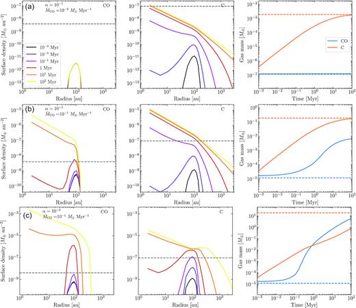
Viscous evolution of a gaseous disc over 100 Myr, with a constant input rate of CO over time and released roughly between 75 and 125 au, for three different cases. Top: high viscosity and low CO input rate. Middle: high viscosity and high CO input rate. Bottom: low viscosity and high CO input rate. The left and middle columns show the evolution of the CO and carbon surface density, respectively. The right column shows the evolution of the total gas mass of CO (blue continuous line) and carbon (orange continuous line). The dashed blue and orange lines represent the CO and carbon mass expected in steady state when CO is unshielded and the mass input rate of CO is constant over time.

Open in new tab Download slide

The top panel shows a simple case that would be applicable to systems that are observed to have a low CO gas mass (e.g. β Pic, HD 181327, and Fomalhaut, Dent et al. 2014; Marino et al. 2016; Matrà et al. 2017b). CO is input in the system and in a few hundred years it reaches steady state with |$\Sigma _\mathrm{CO}=\dot{\Sigma }^{+}_\mathrm{CO} \times 120\ \mathrm{yr}$| and thus is confined in space and co-located with planetesimals and large dust grains (top left). Carbon instead viscously spreads forming an accretion disc which reaches a steady state in a few times the viscous time-scale at the belt location (⁠|$t_\nu =r_\mathrm{belt}^2/\nu =0.6$| Myr, top middle). Neither the surface density of CO nor C reach the necessary levels to shield CO (grey dashed lines), except for carbon within a few au where no CO is present. The final CO and C mass (top right) are consistent with analytic predictions where |$M_\mathrm{CO}=\dot{M}_\mathrm{CO}\times 120\ \mathrm{yr}$| and M_C calculated by integrating equation (B17) in Metzger, Rafikov & Bochkarev (2012) assuming that the viscosity scales linearly with radius (true for our case if μ is constant),

$$\begin{eqnarray*} M_\mathrm{C}= \frac{2 \dot{M}_\mathrm{CO} r_\mathrm{belt}^2 }{7 \nu _\mathrm{belt}} \left[ 2 \left(\frac{r_{\max }}{r_\mathrm{belt}} \right)^{1/2}-1 \right] , \end{eqnarray*}$$

(9)

where r_max is the maximum radius in the simulation. Note that |$M_\mathrm{C}\propto r_{\max }^{1/2}$|⁠, thus the total mass reported here is dominated by low-density gas at large radii to which observations can be less sensitive. Therefore, the carbon masses reported in this section cannot be compared directly with observations. Later in Section 3, we report instead the CO and carbon masses within 500 au which is a more sensible estimate to compare with typical observations. Note that if the viscosity did not scale linearly with radius, then the bulk of the mass could reside at small radii.

In the middle panels, the CO mass input rate is now 100 times higher. While the CO is slightly self-shielded within the first 0.1 Myr of evolution (note that the blue line in the right-hand panel is above the dashed line), by 1 Myr the surface density of carbon reaches the critical level to shield CO at 100 au. The subsequent evolution has CO viscously spreading inwards forming an accretion disc and slightly diffusing outwards, although it is truncated at ∼170 au where the CO lifetime becomes much shorter than the viscous time-scale. Over time the carbon mass increases similarly to the upper panel, although the carbon mass saturates at a slightly lower level than the theoretical maximum because some of the CO is never photodissociated into carbon and oxygen (⁠|${\sim}15\, {\rm per\, cent}$|⁠).

In the lower panels, we show a case with a low viscosity and high CO mass input rate. Due to the lower viscosity, carbon is locally piling up and so reaching a higher surface density much faster than it can spread out. By 0.1 Myr CO becomes shielded by carbon and starts to build-up and viscously spread. With CO’s significantly longer lifetime, the production rate of carbon is much lower, and the mass of CO overcomes the carbon mass after 1 Myr. Nevertheless, the carbon surface density is still comparable to the high viscosity case near the belt location, but orders of magnitude larger beyond 100 au. This means that CO can also significantly spread outwards since it is shielded out to 1000 au, although the viscous time-scale to reach those regions can be shorter than its lifetime. Given the longer viscous time-scale at r_belt (60 Myr), only by the end of the simulation the surface density of CO and carbon is close to steady state at the belt location. Something worth noticing in this last scenario is that the surface density of carbon after 10 Myr has a flat slope in between from r_belt out to where the CO surface density drops exponentially. In the two cases where CO becomes shielded, we find that CO spreads inwards reaching our simulation boundary at 1 au, and spreads outwards out to a radius where its lifetime against photodissociation (determined by both carbon and CO surface densities) is too short for CO to viscously spread or diffuse from where it is produced.

The CO and carbon evolution presented here is overall consistent with the 0D model presented in Kral et al. (2019, see their fig. 18). The main difference is that the predicted masses of carbon and CO (when completely shielded) are overall larger in this study for the same α since in Kral et al. (2019) we used the local viscous time-scale which is a twelfth of the viscous time-scale. Moreover, here we are considering the total gas mass in the system, which can be orders of magnitude higher than the gas mass around the belt location. Therefore, the disc mass saturates at a lower level in our previous simulations and in a shorter time-scale.

2.2 Collisional evolution

An important ingredient that so far has not been considered in previous gas evolution studies (e.g. Kral et al. 2016, 2017, 2019) is the disc collisional evolution. These have assumed that CO gas is released at a constant rate equal to the product between the CO mass fraction in planetesimals, f_CO, and the mass-loss rate due to collisions |$\dot{M}$|⁠. While the first might stay constant over time if planetesimals do not devolatize, the second typically decreases with time (e.g. Dominik & Decin 2003; Krivov, Löhne & Sremčević 2006; Thébault & Augereau 2007; Wyatt et al. 2007a; Löhne, Krivov & Rodmann 2008; Kral, Thébault & Charnoz 2013) as planetesimals are ground down and mass is removed from the system through the blow out of small grains (Burns, Lamy & Soter 1979). Since the rate at which planetesimals suffer disruptive collisions is proportional to the total disc mass, M, it is easy to show that when assuming a single slope size distribution the disc mass should decrease with time as 1/t, with

$$\begin{eqnarray*} M(t) &=& \frac{M_0}{t/t_\mathrm{c}+1}, \\ \dot{M}(t)&=& - \frac{M(t)^2}{M_0t_\mathrm{c}}, \end{eqnarray*}$$

(10),(11)

where t_c is the collisional lifetime of the largest planetesimals at t = 0 and M₀ is the initial disc mass. Note that t here represents the time since planetesimals were stirred enough to cause catastrophic collisions. Here, we assume debris discs are pre-stirred and collisions start immediately after the protoplanetary disc is dispersed.

These equations have two strong implications for the evolution of the disc mass. First, for t ≫ t_c the disc mass will be simply proportional to 1/t and independent of M₀. Thus two systems could have similar masses today although one started its evolution with a much higher disc mass than the other. Therefore the total gas mass released into the system over time can be orders of magnitude different depending on the initial conditions. Secondly, the mass-loss rate decreases as t⁻², which is much faster than the t^−1/2 and t^−3/2 expected for the total mass and surface density of a gaseous disc that evolves viscously according to equation (1) (without input sources). This means that the amount of gas in a debris disc can be out of equilibrium given its current gas release rate which has been decreasing with time.

The collisional lifetime is a function of the initial disc mass and other parameters such as the planetesimal strength, |${Q_\mathrm{D}^{\star }}$|⁠, maximum planetesimal size, D_c, mean eccentricity, e, mean inclination, I, disc mean radius, r, and width, dr. More generally, t_c is given by (Wyatt et al. 2007b)¹

$$\begin{eqnarray*} t_\mathrm{c}=\frac{3.8\rho r^{7/2} (dr/r) D_\mathrm{c}}{M_\star ^{1/2} M}\frac{8}{9 G(X_\mathrm{c}, q)}, \end{eqnarray*}$$

(12)

in years, where ρ is the internal density of solids in kg m⁻³, r and dr are units of au, D_c is in units of km, M_⋆ is in units of M_⊙. G(X_c, q) is a factor defined by equation (10) in Wyatt et al. (2007b) that is a function of q (mass distribution exponent, N(m) ∝ m^−q) and X_c = D_cc/D_c, with D_cc as the size of the smallest planetesimal that has sufficient energy to destroy a planetesimal of size D_c. Its value depends on the relative velocities and |${Q_\mathrm{D}^{\star }}$|⁠, and can be written as (Wyatt & Dent 2002)

$$\begin{eqnarray*} X_\mathrm{c}=1.3\times 10^{-3} \left(\frac{{Q_\mathrm{D}^{\star }}r M_\star ^{-1}}{1.25e^2+I^2} \right)^{1/3}, \end{eqnarray*}$$

(13)

with |${Q_\mathrm{D}^{\star }}$| in units of J kg⁻¹. Assuming ρ = 2700 kg m⁻³, I = e, and X_c ≪ 1, q = 11/6, then |$G\approx 6.5\times 10^{6} [{Q_\mathrm{D}^{\star }}r/(M_\star e^2)]^{-5/6}$| and t_c can be written more simply as

$$\begin{eqnarray*} t_\mathrm{c}=1.4\times 10^{-9} r^{13/3} (dr/r) D_\mathrm{c}{Q_\mathrm{D}^{\star }}^{5/6} e^{-5/3} M^{-1} M_\star ^{-4/3}, \end{eqnarray*}$$

(14)

which is the same as equation (16) in Wyatt (2008).

We use equation (12) to calculate t_c and |$\dot{M}(t)$| assuming an internal density of 2700 kg cm⁻³, a maximum planetesimal size D_c = 1 km, eccentricities and inclinations of 0.1, |${Q_\mathrm{D}^{\star }}$| of 330 J kg⁻¹, q = 11/6 (i.e. a size distribution with a power-law index of −3.5) and a fractional disc width of 0.5. Note that this particular choice of parameters is arbitrary, but in Section 3, we will fix these parameters to those chosen in Wyatt et al. (2007b) to fit the infrared excess evolution at 24 and 70 µm in nearby A stars (Rieke et al. 2005; Su et al. 2006), which are the focus of this paper. Finally, we assume a CO mass fraction in planetesimals of 0.1, consistent with levels inferred in Solar system comets (Mumma & Charnley 2011). Using this set of parameters, below we study the evolution of CO and carbon when the initial planetesimal disc mass is 300 or 30 M_⊕ (t_c = 2 and 20 Myr, respectively), and assuming α = 0.1 (Section 2.2.1) and 10⁻³ (Section 2.2.2). This choice of masses is arbitrary, but it helps to illustrate how important the collisional evolution can be for the gas evolution.

2.2.1 High α

In Fig. 2, we show the gas evolution for two discs starting with a total mass of 300 and 30 M_⊕ (10 per cent of which is in CO) in the high viscosity case. In the high initial mass case (top panel), CO becomes self-shielded before carbon reaches the critical mass since the initial mass-loss rate and CO mass input rate are very high (⁠|$\dot{M}_\mathrm{CO}\sim 20$| M_⊕ Myr⁻¹). Both CO and carbon viscously spread within 0.1 Myr, with carbon reaching larger radii, but not high enough surface densities to shield CO at radii larger than 500 au. For this initial mass, t_c = 2 Myr, hence the evolution after a few Myr is characterized by a declining CO mass input rate (1/t²) which cannot support anymore the high CO surface densities reached at t = 1 Myr since the lifetime of CO at the belt location is about 10 Myr. Therefore, the surface density of CO starts to decline, but not as steeply as an exponential decline because the more CO is photodissociated the higher the surface density of carbon which indeed shields CO (negative feedback). By 10 Myr the carbon surface density and CO lifetime peak, after which CO declines steeply approaching a new and less massive quasi equilibrium (see blue dashed line in right-hand panel). Carbon, on the other hand, decreases slowly with time due to accretion. This difference in the lifetime of CO versus carbon could be observed and tested, but at the moment there are not enough observations of carbon to constrain its lifetime.

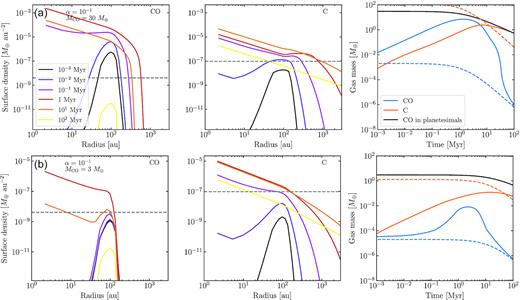
$Same as Fig. 1, but with a CO input rate decaying in time and high viscosity (α = 0.1). Top: initial disc mass of 300 M⊕ with a 10 per cent CO fractional mass. Bottom: initial disc mass of 30 M⊕ with a 10 per cent CO fractional mass. In the right-hand panels, the black line represents the CO mass that is still trapped in planetesimals and which decreases in time as the disc collisionally evolves. The steady state mass represented by dashed lines now decrease with time as the CO mass input rate declines.$

Figure 2.

Same as Fig. 1, but with a CO input rate decaying in time and high viscosity (α = 0.1). Top: initial disc mass of 300 M_⊕ with a 10 per cent CO fractional mass. Bottom: initial disc mass of 30 M_⊕ with a 10 per cent CO fractional mass. In the right-hand panels, the black line represents the CO mass that is still trapped in planetesimals and which decreases in time as the disc collisionally evolves. The steady state mass represented by dashed lines now decrease with time as the CO mass input rate declines.

Open in new tab Download slide

If the starting mass is lower (bottom panel), CO is only slightly self-shielded given the lower CO mass input rate (⁠|$\dot{M}_\mathrm{CO}\sim 0.2$| M_⊕ Myr⁻¹). After 0.1 Myr, the carbon surface density is high enough at 100 au to shield CO and thus the surface density of CO increases until 3 Myr when it reaches its maximum. After a few Myr the CO mass input rate starts declining reducing both the CO and carbon surface densities (although the total carbon mass stays almost constant as the gas viscously spreads to larger radii).

An interesting consequence of the nature of how the mass input rate evolves is that at 100 Myr both scenarios have similar planetesimal disc masses (∼10 M_⊕), and thus also fractional luminosities (f_IR) or dust masses. However, their gas content is not the same because it depends on the mass-loss rate integrated over time and thus there is some memory from their previous state. For example, if we compare the carbon final masses or surface densities, we find that in the high initial mass case they are a factor 10 and 3 larger, respectively. This is because the viscous evolution is slower than the collisional evolution as commented above.

Larger initial disc masses would increase this difference on the gas content even more, while keeping constant the disc mass at 100 Myr, thus unnoticeable from the amount of dust in the system (assuming gas and dust do not interact, see Section 5.6 for a discussion on this). On the other hand, much lower initial masses would result in an evolution with an almost constant |$\dot{M}_\mathrm{CO}$| because it traces M², where M is constant because the lifetime of the largest planetesimals is longer than 100 Myr, thus analogous to the picture presented in Fig. 1(a).

2.2.2 Low α

These differences in the final gas content are more extreme if the viscosity is lower, i.e. if the viscous evolution is slower, thus being even more sensitive to the evolutionary history of the system. As an example, in Fig. 3 we show the evolution of two systems with the same initial masses as in Fig. 2, but with a lower α value. For both examples, CO becomes shielded and stays as such beyond 100 Myr since the viscous time-scale in this case is 60 Myr at r_belt, hence there is not enough time for the gas to viscously evolve and accrete on to the star. Therefore, at 100 Myr the differences in gas masses and surface densities are even larger between the two scenarios. For example, there is an order of magnitude difference in the final CO and carbon masses and CO surface density between the two scenarios. The carbon final surface density, on the other hand, is very similar for both scenarios, with differences only beyond 200 au.

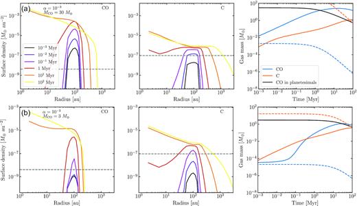
Same as Fig. 2, but with a low viscosity (α = 10−3).

Figure 3.

Same as Fig. 2, but with a low viscosity (α = 10⁻³).

Open in new tab Download slide

Here, we have found that not only the present mass input rate is important, but also the input rate in the past since this is likely to have started at a higher value. This adds a degree of extra complexity to the results shown in Kral et al. (2019, see their fig. 19), where it was shown that the carbon and CO mass depend on the viscosity and CO input rate (assumed to be constant). Moreover, the systems simulated here are far from a quasi steady state between 10 and 100 Myr, except for CO if the initial mass was low enough for CO to be unshielded in which case its evolution would follow the blue dashed line in Figs 2 and 3. But even in this case, the carbon surface density and mass will be out of equilibrium as the viscous evolution is slower than the fast decline rate of |$\dot{M}_\mathrm{CO}$|⁠. These degeneracies and non-linearity between the model parameters, initial conditions, and subsequent evolution complicate the interpretation of observations of gas in debris discs, especially for shielded cases. Nevertheless, population studies can be used as a tool to constrain some of the model parameters by comparing observed and model distributions (see Section 3 below).

3 POPULATION STUDY FOR A STARS

In this section, we study the gas component of a sample of A stars through population synthesis. This approach is ideal for degenerated problems such as the unknown initial disc mass of a particular system, and can provide constraints on population properties. Our population synthesis model simulates the collisional evolution of their planetesimal discs and how the released gas would evolve in those systems. Here, we use the results from Wyatt et al. (2007b) that used the same collisional evolution model to fit the observed distribution of disc temperatures and evolution of infrared excess (or f_IR) around A stars. Wyatt et al. used the distribution of observed 24 and 70 µm excess as a function of age to constrain the initial distribution of disc radii (approximating grains by blackbody spheres) and the maximum f_IR that a disc of a given age and radius can have. The latter is determined by planetesimal intrinsic properties and level of stirring. In particular, they assume all systems are born with a debris disc with a random blackbody radius between 3 and 120 au with a power-law distribution N(r) ∝ r^γ with γ = −0.8 and initial mass following a lognormal distribution with a mean of M_mid and a standard deviation of 1.14 dex. Because the initial fractional luminosity of discs is proportional to |$M_\mathrm{mid} D_\mathrm{c}^{-0.5}$| and the maximum fractional luminosity to |$M_\mathrm{mid}t_\mathrm{c}D_\mathrm{c}^{-0.5}$|⁠, Wyatt et al. (2007b) could constrain these products to |$B\equiv M_\mathrm{mid} D_\mathrm{c}^{-0.5}=1.3$| and |$A\equiv D_\mathrm{c}^{1/2} {Q_\mathrm{D}^{\star }}^{5/6}e^{-5/3}=7.4\times 10^{4}$|⁠, respectively, despite the degeneracy that exists between |${Q_\mathrm{D}^{\star }}$|⁠, e, I, D_c, and M_mid.

To study the gas evolution, the main quantity we aim to obtain from previous dust studies is the mass-loss rate since in our model it determines the gas input rate. However, the collisional evolution model used here does not fully constrain the total mass and mass-loss rate of discs. This can be shown using equations (10) and (11), and the products constrained by Wyatt et al. (2007b). We find that |$\dot{M}\propto B M_\mathrm{mid}/A$| for t ≪ t_c and AM_mid/B for t ≫ t_c. This means that fixing A and B does not fully constrain |$\dot{M}$|⁠, but further assumptions need to be made. Because the gas evolution is very sensitive to |$\dot{M}$|⁠, one could try to vary D_c or M_mid to fit gas observations, but these parameters are degenerated with the fraction of CO in planetesimals. For example, increasing M_mid would increase the CO mass input rate generating larger gas masses, which could also be achieved by increasing the fraction of CO in planetesimals, or alternatively lowering the viscosity. Note that in principle, under certain assumptions one can estimate |$\dot{M}$| from the disc radius, emitting area (or fractional luminosity) and the mass of the particles that contribute the most to the disc’s cross-sectional area (e.g. Matrà et al. 2017b, Appendix B), without making assumptions about the large planetesimals in the disc. We discuss such an approach in Section 5.7. In this section, we keep M_mid fixed to a default value and in Section 5.7, we show that our choice is roughly consistent with inferred mass-loss rates from the dust emission.

Here, we make two subtle changes to the relations that define A and B. First, we introduce a correction factor Γ which is the ratio between the true disc radius over the blackbody radius. This is necessary since the previous study used the blackbody radius (r_BB) when calculating collisional time-scales (since it is the dust temperature which is fitted), which usually differs significantly from the true disc radius being on average underestimated (Booth et al. 2013; Pawellek et al. 2014; Pawellek & Krivov 2015). The difference is due to small grains that tend to have higher temperatures than blackbody spheres, therefore their distance to the star is usually underestimated when fitting blackbody models to SEDs (note that the model in Section 2.2 is based on the true radius). Since the initial fractional luminosity is proportional to |$r_\mathrm{belt}^{-2}$|⁠, and the maximum fractional luminosity to |$r_\mathrm{belt}^{-2}$| and t_c (with |$t_\mathrm{c}\propto r_\mathrm{belt}^{13/3}$|⁠), with the introduction of Γ, we obtain

$$\begin{eqnarray*} D_\mathrm{c}^{1/2}\ {Q_\mathrm{D}^{\star }}^{5/6}\ e^{-5/3}\ \Gamma ^{7/3} &=& 7.4\times 10^{4},\\ M_\mathrm{mid} D_\mathrm{c}^{-1/2} \Gamma ^{-2} &=& 1.3 \end{eqnarray*}$$

(15),(16)

which is the same as used in Kains, Wyatt & Greaves (2011).

Secondly, the planetesimal strength can be parametrized as a function of planetesimal size, with |${Q_\mathrm{D}^{\star }}\propto D_\mathrm{c}^{b_g}$| for planetesimal sizes above a few hundred meters (gravity dominated). For example, for compact planetesimals with sizes larger than a few hundred meters, simulations by Benz & Asphaug (1999) show |${Q_\mathrm{D}^{\star }}=330 D_\mathrm{c}^{1.36}$|⁠. We will take this value as reference, although |${Q_\mathrm{D}^{\star }}$| could be significantly lower if planetesimals are made of aggregates (see Krivov et al. 2018, and references therein). This change assumes however that the collisional evolution can still be approximated by q = 11/6 and equation (10) where t_c is the lifetime of the largest body.

With these changes and a fixed value of Γ, the general evolution of fractional luminosities is left with only one degree of freedom, e.g. fixing e or M_mid leaves completely constrained the rest of the parameters. For Γ = 1 and assuming e = 0.05, we have the canonical values D_c = 4.7 km, |${Q_\mathrm{D}^{\star }}=2700$| J kg⁻¹, and M_mid = 2.8 M_⊕, which are equivalent to the ones used in Wyatt et al. (2007b). For an arbitrary value of Γ and e we have for A stars

$$\begin{eqnarray*} M_\mathrm{mid} &=& 1.7 \left(\frac{e}{0.01}\right)^{0.5} \left(\frac{\Gamma }{1.7}\right)^{1.2} \mathrm{ M}_\oplus ,\\ D_\mathrm{c} &=& 0.2 \left(\frac{M_\mathrm{mid}}{1.7}\right)^2 \left(\frac{\Gamma }{1.7}\right)^{-4} \mathrm{km}. \end{eqnarray*}$$

(17),(18)

Here, we assume Γ = 1.7 which is in the middle of the observed range for A stars (1–2.5, Matrà et al. 2018b), and adopt the following values as standard: D_c = 0.02 km, |${Q_\mathrm{D}^{\star }}=1.6$| J kg⁻¹ and M_mi_d = 0.5 M_⊕ and e = 0.001. Note that there are strong degeneracies between these parameters, and thus these cannot be interpreted physically. The values used here are chosen such that the mass-loss rate in the discs that we model is roughly consistent with the mass-loss rate inferred from their fractional luminosity (see Section 5.7).

We now proceed with these parameters and generate a random sample of 8000 A stars. The mass of each star is randomly chosen between 1.7 and 3.4 M_⊙ and its corresponding luminosity estimated using the mass–luminosity relation. The total disc mass is drawn from a lognormal distribution centred at M_mid and with a standard deviation of 1.14 dex as in Wyatt et al. (2007b). The planetesimal strength, mean eccentricity, and maximum size are set to the values defined above, and we assume a CO mass fraction of 0.1. The disc radii are drawn following a power-law distribution of exponent –0.8 and with a minimum and maximum radius of 5.1–204 au, consistent with Wyatt et al. (2007b) when Γ is set to a value of 1.7. Finally, we assume exocometary gas release starts at an age of 3 Myr (i.e. shortly after protoplanetary disc dispersal) and we evolve systems up to a random age between 3 and 100 Myr to get an age spread and we keep the value of α fixed to 0.1 (Section 3.1) or 0.001 (Section 3.2).

In the following Sections 3.1 and 3.2, we compare the model distributions of CO and carbon masses to observations of a sample of A stars. To do so, it is important to first consider biases of any selected sample. We choose to compare our results with the complete sample of A stars within 150 pc that have been targeted by ALMA, and that meet the following criteria (Moór et al. 2017, the most complete study of gas around A stars with debris discs): (i) disc fractional luminosity between 5 × 10⁻⁴ and 10⁻²; (ii) dust temperature below 140 K; (iii) detection at ≥70 µm with Spitzer or Herschel; and (iv) age between 10 and 50 Myr. We apply the same filtering process to our synthesized sample to do a fair comparison between model and observations. In this way both observed and model samples have the same biases. In the following sections, we present both whole and filtered model populations, representing them with small dots and blue contours, respectively.²

3.1 High α

In Fig. 4, we present the distribution of the initial disc mass (M₀), final CO mass contained within 500 au (at a random age between 3 and 100 Myr), and the final surface density of CO and carbon at the belt location, that result from our simulations. We overlay in blue contours the distribution of systems that would have been selected by Moór et al. (2017). We find that the distributions of some parameters are highly correlated as expected. First, the more massive the initial disc mass is, the higher the amount of CO and carbon gas that will be present at a later epoch. For initial disc masses higher than ∼10 M_⊕, the CO mass distribution of the filtered sample extends to much higher values as CO becomes shielded. This is also true for the full population, but it is harder to see due to the age and radius spread which means that small warm discs with low initial masses can also reach shielded states for a short period. On the other hand, the surface density of carbon never reaches values as high as CO because the more carbon there is, the more CO is shielded and thus the lower carbon production rate.

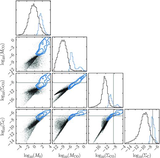
Distribution of the initial disc mass M0, final CO mass MCO, and final surface density of CO and carbon. The contours represent regions that enclose the 68 per cent, 95 per cent, and 99.7 per cent of the distribution of the filtered population. The grey lines represent the critical surface density over which CO and carbon can shield CO from UV photons. All variables are in units of M⊕ or M⊕ au−2. The marginalized distributions in the top panels are shown at an arbitrary scale for display purposes.

Figure 4.

Distribution of the initial disc mass M₀, final CO mass M_CO, and final surface density of CO and carbon. The contours represent regions that enclose the 68 per cent, 95 per cent, and 99.7 per cent of the distribution of the filtered population. The grey lines represent the critical surface density over which CO and carbon can shield CO from UV photons. All variables are in units of M_⊕ or M_⊕ au⁻². The marginalized distributions in the top panels are shown at an arbitrary scale for display purposes.

Open in new tab Download slide

The top panel of the second column shows the distribution of CO. While the bulk of the population is unshielded, the distribution has a tail extending to larger masses, with a small fraction (2 per cent) having CO masses between 10⁻⁴ and 1 M_⊕ (the typical CO masses derived for shielded discs, Moór et al. 2017) or carbon surface densities at the belt location above the critical value to shield CO (4 per cent). We find that applying the same selection mentioned above filters 99 per cent of systems. Of the remaining 1 per cent, 33 per cent have CO masses higher than 10⁻⁴ M_⊕ displaying a bimodal distribution, and 49 per cent have carbon surface densities above the critical value. These numbers are both consistent with the number of A stars that meet the selection criteria (17 of ∼8000 main-sequence A stars within 150 pc) and with the statistics for shielded discs (i.e. 9/17 systems with CO masses ≳10⁻⁴–1 M_⊕, Bovy 2017; Moór et al. 2017).

As expected, discs with large CO masses all have carbon surface densities above which shielding by carbon becomes important (grey lines). Note that there are no discs that are self-shielded but with carbon surface densities below the critical value. The reason for this can be understood by assuming quasi-steady state. Consider a disc with a constant input rate |$\dot{M}_\mathrm{CO}$|⁠. The minimum CO mass input rate such that CO is self-shielded is |$\Sigma _\mathrm{CO,c} \pi r_\mathrm{belt}^2/T_\mathrm{ph}$| (assuming CO does not viscously spread and Δr_belt/r_belt = 0.5), while the minimum to reach carbon shielding is |$7\Sigma _\mathrm{C,c}\pi \nu _0 r_\mathrm{belt}$| (where ν = ν₀r, Metzger et al. 2012). By equating these two expressions, we find that shielding by carbon will be more important in debris discs larger than

$$\begin{eqnarray*} r_\mathrm{c}=7\ T_\mathrm{ph} \nu _0 \frac{\Sigma _\mathrm{C,c}}{\Sigma _\mathrm{CO,c}}, \end{eqnarray*}$$

(19)

which evaluated for α = 0.1 gives 3 au (lower than the 5 au minimum disc radius considered here). Therefore, it is very unlikely to observe a disc in the bottom right corner of the intersection between the grey lines, i.e. only self-shielded. Lower viscosities will make r_c even lower. A caveat in this estimate is that for mass input rates much higher than the minimum to become shielded, at early times CO might become self-shielded before becoming shielded by carbon as shown in Fig. 2.

In order to understand what is the dependence of the CO mass with the age, belt radius, and fractional luminosity of a system, Fig. 5 shows the scatter of these parameters for each simulated system and their distribution in blue when applying the selection criteria commented above. As a comparison, the red circles and triangles represent the CO detections and upper limits around A stars that meet the selection criteria (Kral et al. 2017; Moór et al. 2017; Kennedy et al. 2018; Booth et al. 2019; Hales et al. 2019, see table A1). For the non-detections around HD 98363, HD 109832, HD 143675, and HD 145880 we use the non-LTE tool from Matrà et al. (2018a) to compute CO mass upper limits, assuming kinetic temperatures of 150 K and a radial distance of 1.7 their dust blackbody temperatures (their belts have not been resolved). The top panel shows M_CO versus age. This distribution reveals how the fraction of systems with large CO gas masses decreases with time and by 50 Myr less than 1 per cent of the whole population remain with CO masses higher than 10⁻⁵ M_⊕. The time-scale at which shielded discs disappear is related to how fast gas viscously evolves, thus a smaller viscosity would result in long-lasting shielded discs as discussed in Section 2.2.2. Note that the distribution of red dots is consistent with the blue density map, and we do not expect CO masses lower than 10⁻⁷ M_⊕, which depending on line excitation conditions is at the limit of typical deep ALMA observations (e.g. Marino et al. 2016; Matrà et al. 2017b), but below the sensitivity of shallow CO surveys (e.g. Kral et al. 2017; Moór et al. 2017). Hence given the above selection cuts, the distribution of CO gas masses inferred from observations is consistent with our model. It is also worth mentioning that the CO mass estimates shown here have uncertainties that typically are an order-of-magnitude wide.

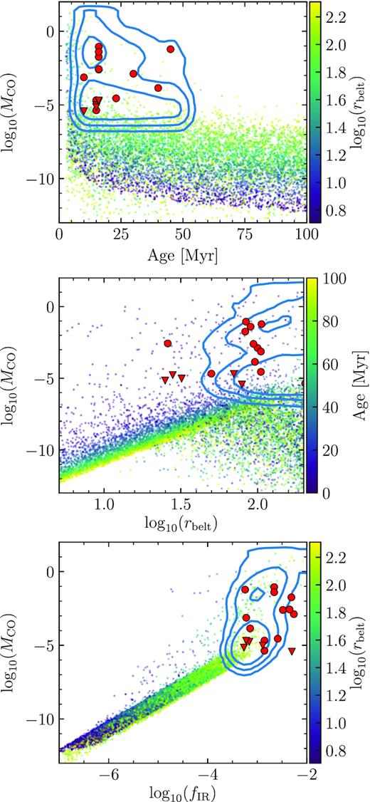
$Population synthesis for A stars with α = 10−1. Top: CO gas mass (MCO) in M⊕ versus age. Middle: CO gas mass versus radius. Bottom: CO gas mass versus disc fractional luminosity. Each point corresponds to a different simulation. The contours represent regions that enclose the 68 per cent, 95 per cent, and 99.7 per cent of the distribution of the filtered population. The red circles and triangles represent the CO detections and upper limits around A stars that meet the same selection criteria as the filtered population.$

Figure 5.

Population synthesis for A stars with α = 10⁻¹. Top: CO gas mass (M_CO) in M_⊕ versus age. Middle: CO gas mass versus radius. Bottom: CO gas mass versus disc fractional luminosity. Each point corresponds to a different simulation. The contours represent regions that enclose the 68 per cent, 95 per cent, and 99.7 per cent of the distribution of the filtered population. The red circles and triangles represent the CO detections and upper limits around A stars that meet the same selection criteria as the filtered population.

Open in new tab Download slide

The middle panel of Fig. 5 shows the distribution of M_CO versus r_belt. We find that the bimodal distribution of M_CO discussed above is present across the whole distribution of r_belt, and can be split into three populations, two with low CO masses and one with shielded and massive CO discs. For those systems that are unshielded, CO mass seems to increase with radius up to r_belt ∼ 50 au after which the median CO mass decreases with radius. This is expected given that the CO mass in the unshielded case is simply proportional to the mass-loss rate, which for t ≫ t_c is proportional to t_c ∝ r^13/3 (equation 14), whereas for t ≪ t_c is proportional to 1/t_c ∝ r^−13/3. The transition happens where t_c ∼ 50 Myr (mean system age), which using M_mid we find this should happen at r_belt ∼ 56 au. The larger dispersion for discs with a large radius is due to the mass input rate being proportional to |$M_0^2$| (for t ≪ t_c) which has a large dispersion. The third population is composed of shielded discs that exists predominantly in young systems with a high initial mass and with a large disc radius. We find that the distribution of observed discs matches reasonably well the expected distribution, with the exception of HD 121191, whose belt has not been resolved with enough sensitivity (we used 1.7 times its blackbody radius, which could be easily an underestimate, Moór et al. 2017), thus it could be significantly larger than the value used here.

The bottom panel of Fig. 5 shows the distribution of M_CO versus fractional luminosity (f_IR). The fractional luminosity is calculated using equations (14) and (15) in Wyatt (2008), but using the blackbody radius instead of the true radius. For f_IR ≲ 10⁻⁴, we find that M_CO is roughly proportional to |$f_\mathrm{IR}^2$|⁠, a result that is expected since the CO release rate and mass-loss rate in a belt is proportional to the square of the mass or |$f_\mathrm{IR}^2$|⁠. On the other hand, for larger f_IR the CO masses grow steeply with fractional luminosity since CO is shielded in these systems. Overall, the observed distribution (red dots) is consistent with the filtered model population (blue contours) given the typical uncertainties in gas masses (∼1 dex). The big exception is HR 4796. The CO mass upper limit for this system is below the blue 3σ confidence region by orders of magnitude. This disc has one of the highest fractional luminosities and is very narrow, hence the CO release rate should be high. Kennedy et al. (2018) concluded that the planetesimals must have a CO + CO₂ ice mass fraction below 2 per cent. This is discussed further in Section 5.1.1.

Finally, in the top panel of Fig. 6 we compare the carbon and CO masses of our models (contained within 500 au) with the estimated CO and neutral carbon mass in four discs (β Pic, 49 Ceti, HD 131835, HD32297, Higuchi et al. 2017, 2019; Cataldi et al. 2018; Cataldi et al. 2019; Kral et al. 2019). Overall, we find that the observed carbon masses are lower than predicted by our model. This has been highlighted recently by Cataldi et al. (2018, 2019) and used to argue in favour of a scenario in which gas was released only recently in the β Pic and HD 32297 systems. This comparison is difficult since most of the carbon mass resides at large radii where typically ALMA observations are less sensitive (due to the primary beam and low-surface densities). This is why we report gas masses as the total masses contained within 500 au, as a proxy for the observable mass. Note that this affects more the carbon mass than the CO mass, since carbon is always distributed up to larger radii. In steady state, we expect the total carbon mass to be proportional to |$r_{\max }^{1/2}$| for r_max > r_belt (equation 9), so the observable mass could vary by a factor of a few if we used a different definition. This together with the low number statistics, unknown ionization fraction (see Section 5.1.2) and uncertain excitation conditions for the observed lines, hinders any strong conclusions on the model success at reproducing observations. If the carbon mass was indeed lower than predicted by our model, this could be due to a higher viscosity, however this would lower the CO mass of shielded discs in our model (lower shielding and shorter viscous time-scale) making it inconsistent with observations. Alternatively, we can estimate an observable carbon mass as the product between the carbon surface density at the belt location times the area of the belt, i.e. |$\Sigma _{\mathrm{C},r_\mathrm{belt}} \pi r_\mathrm{belt}^2$| (for a fractional width of 0.5). This is shown in the bottom panel of Fig. 6. Using this definition for carbon mass, we find a better agreement with observations. This illustrates that simple comparisons between model and observations are difficult. We identify the gas surface density at the belt location as a better quantity to test shielding models, since it is the vertical column densities of carbon and CO that set the CO photodissociation time-scale in this context. Note that estimating the neutral carbon surface density from current observations is very difficult since the observed systems were edge-on (β Pic and HD32297) or marginally resolved (HD 131835). Moreover, the observed single carbon line in some of these systems is close to being optically thick and degenerate with excitation conditions, hindering determining the total carbon mass present (49 Ceti).

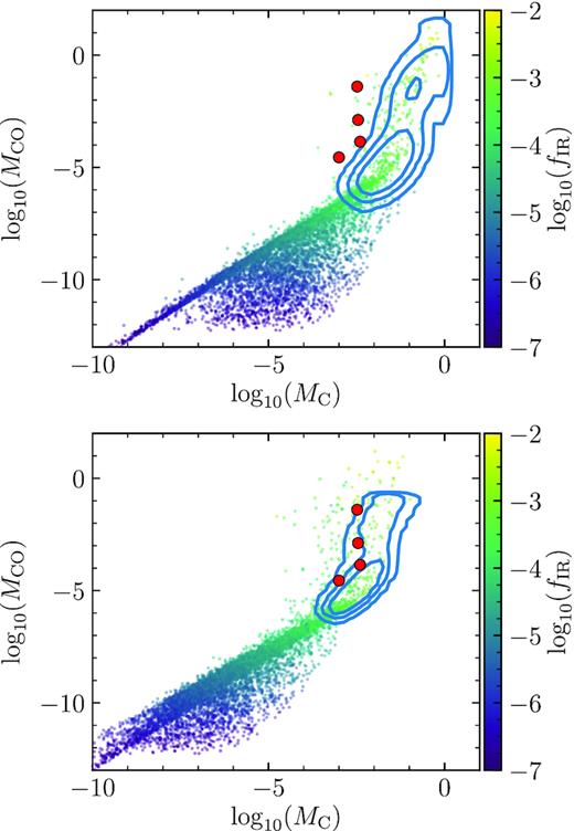
$Population synthesis model for the carbon and CO masses around A stars assuming a high viscosity (α = 0.1). Top: The carbon model mass represents all mass within 500 au. Bottom: The carbon model mass is calculated as $\Sigma _{\mathrm{C},r_\mathrm{belt}} \pi r_\mathrm{belt}^2$. Each point corresponds to a different simulation. The contours represent regions that enclose the 68 per cent, 95 per cent, and 99.7 per cent of the distribution of the filtered population. As a comparison, the red circles represent the CO and carbon detections around A stars that meet the same selection criteria as the filtered population.$

Figure 6.

Population synthesis model for the carbon and CO masses around A stars assuming a high viscosity (α = 0.1). Top: The carbon model mass represents all mass within 500 au. Bottom: The carbon model mass is calculated as |$\Sigma _{\mathrm{C},r_\mathrm{belt}} \pi r_\mathrm{belt}^2$|⁠. Each point corresponds to a different simulation. The contours represent regions that enclose the 68 per cent, 95 per cent, and 99.7 per cent of the distribution of the filtered population. As a comparison, the red circles represent the CO and carbon detections around A stars that meet the same selection criteria as the filtered population.

Open in new tab Download slide

3.2 Low α

Using the same collisional evolution model as in the previous section, we use a lower α = 10⁻³ and make predictions for the mass of CO and carbon for a population of systems around A stars. Fig. 7 shows the results for the CO mass as a function of age (top), r_belt (middle), and f_IR (bottom). We find a stronger bimodal distribution compared to the results with a high α. A larger fraction of systems become shielded and stay almost constant in time because the viscous evolution time-scale for these discs is 100 times longer. Moreover, the CO masses of shielded discs are much higher because accretion is slower, and inconsistent with the observations (compare the blue contours with the red markers). In fact, even discs with low fractional luminosities which would have been undetectable with Spitzer or Herschel have high levels of shielded CO which hints at their high initial masses and fast collisional evolution. Because viscosity is low, CO gas takes much longer to disappear compared to solids. Therefore, the model in this paper disfavours low viscosities. Nevertheless, unbiased searches for CO have not been done around nearby A stars, thus we cannot rule out the presence of massive gas discs around stars without detectable debris discs.

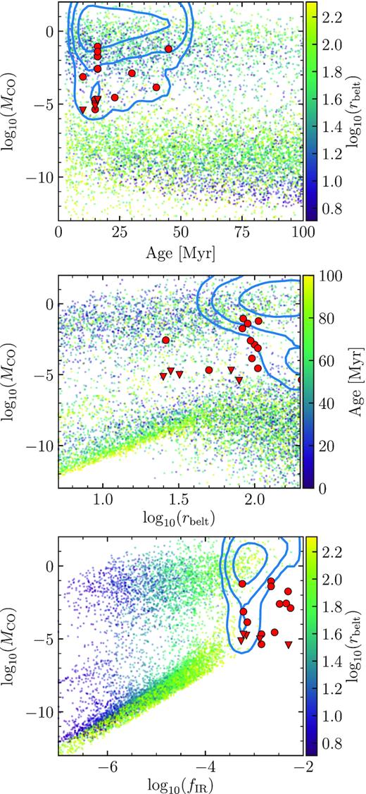
$Population synthesis for A stars with α = 10−3. Top: CO gas mass (MCO) in M⊕ versus age. Middle: CO gas mass versus radius. Bottom: CO gas mass versus disc fractional luminosity. Each point corresponds to a different simulation. The contours represent regions that enclose the 68 per cent, 95 per cent, and 99.7 per cent of the distribution of the filtered population. The red circles and triangles represent the CO detections and upper limits around A stars that meet the same selection criteria as the filtered population.$

Figure 7.

Population synthesis for A stars with α = 10⁻³. Top: CO gas mass (M_CO) in M_⊕ versus age. Middle: CO gas mass versus radius. Bottom: CO gas mass versus disc fractional luminosity. Each point corresponds to a different simulation. The contours represent regions that enclose the 68 per cent, 95 per cent, and 99.7 per cent of the distribution of the filtered population. The red circles and triangles represent the CO detections and upper limits around A stars that meet the same selection criteria as the filtered population.

Open in new tab Download slide

Because the solid mass-loss rate and thus the CO mass input rate are not fully constrained by the collisional evolution model used here, it might still be possible to fine tune parameters such that with a low viscosity the predicted CO masses are lower. We showed above that the mass input rate of the population is proportional to M_mid or |$D_\mathrm{c}^{0.5}$| (and constants), so in order to reduce the mass input rate by a factor of 100 to counteract the 100 times lower viscosity, we would need to reduce D_c by a factor of 10⁴, and thus also decrease M_mid by a factor 100 and increase |${Q_\mathrm{D}^{\star }}$| by a factor 250. Such a large strength for such small bodies is unrealistic (Benz & Asphaug 1999), thus we conclude that α values as low as 10⁻³ are unlikely to explain the observed properties of gas in high fractional luminosity discs. Moreover, high-gas masses are only found in systems younger than 50 Myr (Greaves et al. 2016), thus favouring a viscous time-scale shorter than 50 Myr at the belt location.

Another source of degeneracy is the assumed CO fraction in planetesimals. A lower CO abundance would lower the input rate of CO, which combined with a low viscosity could still fit the observed distribution of CO masses. This is not explored in this paper, but in Section 5.2.1, we discuss avenues to break these degeneracies using independent observations.

4 SOLAR-TYPE STARS

Exocometary gas is not only found around A stars, but also around lower mass stars, from F to M (Lieman-Sifry et al. 2016; Marino et al. 2016, 2017; Matrà et al. 2019), however high CO mass discs are only found around A stars so far. This could be due to A stars being born with more massive discs on average, which was hinted by Matrà et al. (2019) based on a higher fractional luminosity in the more luminous stars that have been observed with ALMA. Here, we aim to show that shielded discs are unlikely to be found around FGK stars simply because their planetesimal belts are born less massive than their A stars counterpart (or equivalently have a lower |$\dot{M}$|⁠).

We take the same approach as for A stars, and we simulate a population of FGK stars following the results by Sibthorpe et al. (2018) that used both Spitzer and Herschel FIR photometry of 275 FGK stars to fit a collisional evolution model, similar to Wyatt et al. (2007b). That study found best-fitting parameters A = 5.5 × 10⁵, B = 0.1, and γ = −1.7. We assume the same planetesimal strength relation as before, eccentricities of 0.001 and Γ = 3.1 (the average true to blackbody radius ratio for FGK stars resolved by ALMA, Matrà et al. 2018b). Fixing these parameters we have D_c = 0.03 km and M_mid = 0.16 M_⊕ (versus 0.02 km and 0.5 M_⊕ for A stars), i.e. discs around FGK stars are born on average with a lower mass and lower fractional luminosities. We can anticipate that FGK stars will have lower mass CO discs, and for the same α value used here (0.1) viscosities will be slightly lower (a factor ∼2) due to the different stellar masses and luminosities. We simulate then 8000 FGK stars with stellar masses between 0.56 and 1.6 M_⊙, blackbody radius between 1 and 1000 au (i.e. real radius between 3.1 and 3100 au), and ages between 3 and 100 Myr. Note that this large upper limit on the disc radius beyond 500 au is unrealistic given the observed population of debris and protoplanetary discs. Moreover, temperatures beyond 500 au might be below the CO sublimation temperature and thus CO would not be released. We keep this large upper limit because if not there is no guarantee that the model distribution would still fit the distribution of fractional luminosities of FGK stars. Nevertheless, because of the low value of γ only a very small fraction of simulated systems have radii larger than 500 au. Therefore, this unrealistic choice of upper boundary in the radius distribution does not affect our conclusions.

Similar to the previous figures, we present in Fig. 8 the distribution of CO masses versus age, belt radius, and fractional luminosity. We find that overall the CO masses of the population are much lower, even after applying the same selection cuts as for A stars (blue contours, 2 per cent of the whole population). This is because for a fixed fractional luminosity, the gas release rate is higher for more luminous stars (Matrà et al. 2019). We find that only 1 per cent of the whole fraction has CO masses above 10⁻⁴ M_⊕, most of which are young systems with small discs. This fraction only grows to 4 per cent for the filtered population. When we look instead at the carbon surface density at the belt location, we find that only 3 per cent is above the critical value to shield CO, and this number increases only to 11 per cent in the filtered population. Note that the filtered population is consistent with observations of FGK stars with bright debris discs represented by red circles and triangles (see Table A2). Our model then explains why we do not find hybrid/shielded discs around FGK stars as they are not as common given the collisional evolution models that fit their infrared excesses.

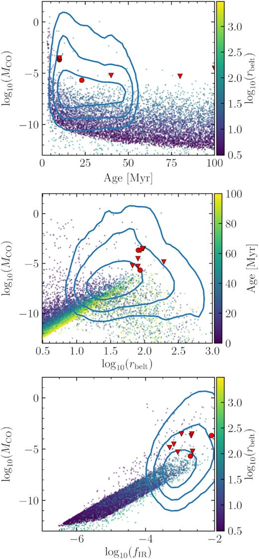
$Population synthesis for FGK stars with α = 10−1. Top: CO gas mass (MCO) in M⊕ versus age. Middle: CO gas mass versus radius. Bottom: CO gas mass versus disc fractional luminosity. Each point corresponds to a different simulation. The contours represent regions that enclose the 68 per cent, 95 per cent, and 99.7 per cent of the distribution of the filtered population. The red circles and triangles represent the CO detections and upper limits around FGK stars that meet the same selection criteria as the filtered population.$

Figure 8.

Population synthesis for FGK stars with α = 10⁻¹. Top: CO gas mass (M_CO) in M_⊕ versus age. Middle: CO gas mass versus radius. Bottom: CO gas mass versus disc fractional luminosity. Each point corresponds to a different simulation. The contours represent regions that enclose the 68 per cent, 95 per cent, and 99.7 per cent of the distribution of the filtered population. The red circles and triangles represent the CO detections and upper limits around FGK stars that meet the same selection criteria as the filtered population.

Open in new tab Download slide

5 DISCUSSION

5.1 Caveats

In this section, we discuss some of the assumptions made in our modelling, when these are justified and how replacing these by more complex models could have an impact on some of our conclusions.

5.1.1 Other volatiles

In this paper, we have focused on the release of CO only. Other volatiles that are abundant in Solar system comets such as H₂O, CO₂, CH₄, HCN, CN, C₂H₆, NH₃, H₂S, etc. could also be released in collisions that expose the interior of planetesimals. This will only happen if temperatures are high enough for thermal desorption (before or after collisions) or if there is a strong UV radiation so photodesorption is effective (Grigorieva et al. 2007). Assuming planetesimals at large radii are similar in composition to Solar system comets, we expect that only water and CO₂ to be as abundant or more than CO so their effect could be important in the model presented here. We expect that water thermal desorption will only be important interior to 10–20 au where blackbody temperatures are higher than 150 K around A stars, although photodesorption could act instead as the release mechanism at large radii. This could mean that the total amount of gas is higher by a factor of a few, but this would not affect the evolution of CO and carbon since the viscous evolution equations are scale independent for the mass and these molecules cannot act as shielding agents because they photodissociate at (UV) wavelengths longer than CO photodissociates and C ionizes. The only noticeable effect on the gas would be that the oxygen to carbon ratio in the disc would be higher, which was used as an argument in Kral et al. (2016) to infer that water is also being released around β Pic, although not detected (Cavallius et al. 2019). On the other hand, including CO₂ would be equivalent to increasing the fraction of CO in planetesimals, since CO₂ is photodissociated into CO and oxygen in a time-scale shorter than CO. Even if neutral carbon is present, it cannot shield CO₂ by more than a factor 0.33 (Rollins & Rawlings 2012), thus whether the CO in the model was released directly from collisions or is a result of CO₂ photodissociation has little effect. The only effect would be that the oxygen to carbon ratio in the disc would be higher, and even more if water is released too. A potential noticeable effect of including other volatile species could be that the higher gas density could increase the gas drag on the dust (see discussion in Section 5.6).

One effect that could be important and neglected here, is that if temperatures of the largest planetesimals are higher than the water sublimation temperature, volatiles might not remain trapped in the interiors and planetesimals could devolatize on short time-scales compared to their collisional lifetime. Therefore, any conclusion on the evolution of gas in discs within 20 au must be taken with caution since gas released might not be controlled by collisional processes (e.g. Marino et al. 2017).

Moreover, in this paper we have assumed a constant CO abundance in planetesimals. This could not be the case since we expect that the CO abundances will depend both on the CO abundance in their progenitors protoplanetary discs, but also on the disc temperature where planetesimals formed. If mid-plane temperatures at formation were close or higher than ∼20 K (CO freeze out temperature), then planetesimals might lack CO. The best example for this possibility is HR 4796, which given that it is an A0 star and its belt is at only 79 au, it could well be that its planetesimals were formed within the CO snowline and thus poor in CO. In fact, HR 4796 is the system with the highest predicted mid-plane temperature at the belt location (see snowline locations in fig. 1 in Matrà et al. 2018b), or smallest radius compared to the CO snowline given its central star. Computing the effect of this temperature dependence on the CO abundance in planetesimals is difficult since it would involve knowledge of the temperatures in the parent protoplanetary disc. In addition, even if planetesimals were CO poor, they could contain large fractions of CO₂ which has a higher freeze out temperature. Therefore CO₂, which photodissociates very quickly and cannot be fully shielded by carbon, could be released producing large quantities of CO gas.

5.1.2 Carbon ionization fraction

Here, we discuss the effect of carbon ionization on the results presented in this paper. This can be important since it is the carbon ionization continuum that can shield CO and explain the observed massive CO discs around A stars. In our model, we neglect the presence of ionized carbon, or in other words we assume that the ionization fraction of carbon is much lower than 1 (i.e. ≲0.3). While carbon ionization can be significant (e.g. in discs with low CO masses like β Pic C⁰/C ∼ 0.015–0.2, Cataldi et al. 2014, 2018), it has only been constrained by observations in one shielded disc (lower than 0.4 in HD 131835, Kral et al. 2019). Here, we aim to show that the ionization fraction is lower than 0.3 for shielded discs, i.e. for discs with a carbon surface density higher than its critical surface density of 10⁻⁷ M_⊕ au⁻².

We calculate the ionization fraction of carbon using equation (15) in Kral et al. (2017), taking into account the stellar and interstellar radiation field (Draine 1978; van Dishoeck, Jonkheid & van Hemert 2006) and assuming an optically thin medium (worst-case scenario). In Fig. 9, we present the ionization fraction as a function of radius and carbon surface density for an A9V (top) and A0V star (bottom). The grey dashed horizontal line represents the critical surface density of neutral carbon for shielding and the continuous white contour represents an ionization fraction of 0.3. Overlaid in white dotted lines, we plot the surface density expected for carbon in steady state (Metzger et al. 2012) if it is being input at 100 au at a rate of 10⁻¹ and 10⁻³ M_⊕ Myr⁻¹ and with α = 0.1. We find that the ionization fraction is always lower than 0.3 when densities are higher than the carbon critical density. Only within 3 au for the A0V star, the ionization fraction is higher than 0.3 for surface densities above the critical value for shielding. Therefore, we conclude that for our 1D model neglecting carbon ionization is a valid assumption for shielded discs.

$Carbon ionization fraction as a function of radius and surface density around an A9V (top) and A0V star (bottom). The horizontal grey dashed line represents the critical density at which neutral carbon starts shielding CO. The white continuous line represents the 0.3 ionization level. The white dotted lines represent the expected surface density for a disc with a high viscosity (α = 0.1) where carbon is being input at 100 au at a rate of 10−1 and 10−3 M⊕ Myr−1.$

Figure 9.

Carbon ionization fraction as a function of radius and surface density around an A9V (top) and A0V star (bottom). The horizontal grey dashed line represents the critical density at which neutral carbon starts shielding CO. The white continuous line represents the 0.3 ionization level. The white dotted lines represent the expected surface density for a disc with a high viscosity (α = 0.1) where carbon is being input at 100 au at a rate of 10⁻¹ and 10⁻³ M_⊕ Myr⁻¹.

Open in new tab Download slide

For low mass gaseous discs, the ionization fraction can be close to one, specially for discs around early-A type stars, although the ionization fractions are likely lower when taking into account the optical depth in the UV. This high-ionization fraction has little effect on the lifetime of CO since it would be vertically unshielded even if all carbon were neutral. Therefore, the evolution of these discs is not dependant on the level of ionization. Note, however that for those discs, the mass of neutral carbon that our model predicts could be overestimated.

A caveat in this calculation is that we are computing the ionization fraction in the disc mid-plane, while the carbon atoms that could shield CO must lie in upper layers. Further work in 2D including the vertical dimension is necessary to estimate more precisely the ionization fraction of carbon in the upper layers, as well as the vertically dependent UV radiation impinging the CO molecules (e.g. Kral et al. 2019). Moreover, here we only considered the photospheric emission, while these stars can have significant additional chromospheric emission in the UV (Matrà et al. 2018a). These considerations require detailed modelling of the stellar emission and are beyond the scope of this paper.

5.1.3 CO photodissociation including stellar UV

Throughout this paper, we have assumed that the photodissociation of CO is controlled purely by UV radiation impinging CO molecules in the vertical direction. This is only valid when the stellar UV flux is lower than the ISRF (e.g. for gas at 100 au around stars with luminosities below ∼20 L_⊙) or if CO is shielded in the radial direction by carbon. We are interested in the second case since this could be common among massive discs independently of the stellar type. In order to check this, we first compare the radial column density of neutral carbon in the radial (towards the star) and vertical direction (from the mid-plane), assuming the following: (i) a disc surface density corresponding to an accretion disc with an input source at a belt radius of 100 au (Metzger et al. 2012); (ii) a disc inner edge at R_⋆ (2.1 R_⊙), 1 and 50 au; (iii) a surface density at 100 au equal to the carbon critical surface density (10⁻⁷ M_⊕ au⁻²); (iv) a disc scale height of 0.05r. Fig. 10 shows these column densities as a function of radius. We find that the radial component is always orders of magnitude larger than the vertical one, even when using a disc inner edge of 50 au.

Figure 10.

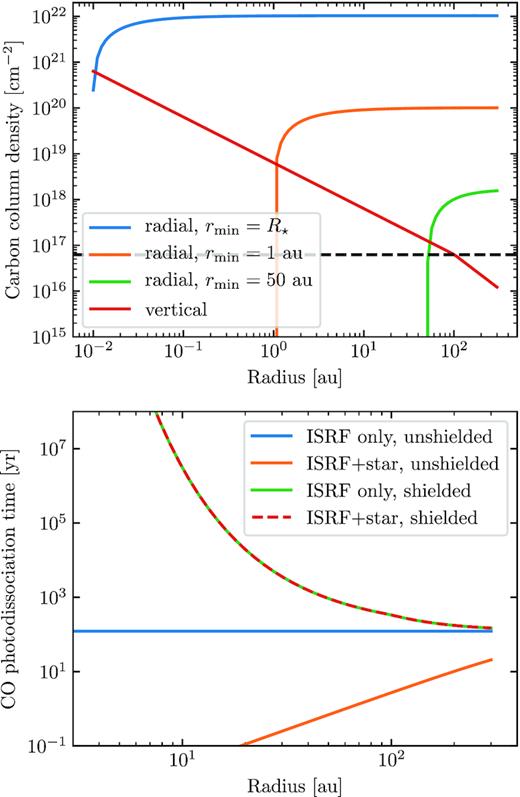
Top: Column density of carbon in the radial (towards the star) and vertical (from the mid-plane, red line) directions. The radial component is shown for three different cases in which the disc inner edge is at the stellar surface (2.1 R_⊙), 1 and 50 au (blue, orange, and green lines). The horizontal dashed black line represents the critical column density of carbon above which it can effectively shield the CO. Bottom: CO photodissociation time-scale assuming a carbon disc extending down to the stellar surface and calculated in four different scenarios: radiation dominated by the ISRF and neglecting shielding (blue), radiation dominated by the ISRF and considering shielding (green), radiation from the ISRF and an A0 star and neglecting shielding (orange line), and radiation from the ISRF and an A0 star and considering shielding (red dashed line).

Open in new tab Download slide

Then, in the case of a disc extending inwards until reaching the stellar surface, we calculate the CO photodissociation rate (Matrà et al. 2018a) around an A0 star considering shielding by carbon only. In the bottom panel of Fig. 10, we compare the photodissociation time-scale of four different cases or assumptions: ISRF only and no shielding; the ISRF plus the stellar radiation and no shielding; the ISRF only and vertical shielding (as in this paper); and the ISRF and stellar radiation and both vertical and radial shielding. We find that as expected, when neglecting carbon shielding (orange line), the photodissociation time-scale is much lower than 120 yr. However, when considering carbon shielding (red and green lines) the photodissociation time-scale is primarily set by the ISRF and vertical shielding. In fact, including the stellar contribution and the carbon shielding along the radial direction does not change significantly the CO photodissociation rate. We find this is true at 100 au even for low neutral carbon surface densities of 3 × 10⁻¹² M_⊕ au⁻², i.e. for all discs in the filtered model population and most of the discs that we model (see bottom right corner in Fig. 4). Therefore, we conclude that for the filtered population it is safe to neglect the stellar UV contribution to the CO photodissociation.

5.2 Breaking degeneracies

5.2.1 Measuring α

As commented in Section 3.2, in our population synthesis model a degeneracy exists between the kinematic viscosity (or α) and the fraction of CO in planetesimals. A potential way to break this is by estimating the level of turbulence in the disc through line observations and thus constraining α independently. Generally speaking, the local line width of an emission line in velocity units (without taking into account Doppler shifts due to Keplerian rotation) is

$$\begin{eqnarray*} \Delta v_\mathrm{line}=\sqrt{2 k_\mathrm{B} T / (\mu m_\mathrm{ p}) + v_\mathrm{turb}^{2}} , \end{eqnarray*}$$

(20)

where T is the gas temperature, μ the mean molecular weight, m_p the proton mass, and v_turb is the turbulent linewidth.³ The turbulent line width can be approximated by |$\sqrt{\alpha } c_\mathrm{ s}$|⁠, thus obtaining |$\Delta v_\mathrm{line}=c_\mathrm{ s}\sqrt{2+\alpha }$|⁠, where c_s is the sound speed. Therefore, if we can constrain c_s from the disc scale height or temperature (e.g. through line excitation temperature, line brightness from optically thick emission or dust observations), then α could be constrained independently from our population synthesis model, allowing to constrain the fraction of CO in planetesimals. This idea is not new, and multiple studies exist in protoplanetary discs trying to constrain α through line observations (e.g. Hughes et al. 2011). The difference here is that a larger α value compared to protoplanetary discs should be easier to observe and the vertical dependence of the temperature should be weaker since these discs are optically thin.

In order to constrain α to values near 0.1, it would be necessary to constrain the line FWHM with a precision below 1 per cent, which is achievable with high-S/N observations that can resolve the line intrinsic widths. The precision or fractional uncertainty on the line FWHM can be written as (Lenz & Ayres 1992)

$$\begin{eqnarray*} \frac{\sigma _\mathrm{FWHM}}{\mathrm{FWHM}} = 1.4 \sqrt{ \frac{ \Delta v}{ \mathrm{FWHM} }} \frac{1}{\mathrm{(S/N)}_0}, \end{eqnarray*}$$

(21)

where Δv is the spectral resolution and (S/N)₀ is the S/N at the line peak. Since the peak S/N typically scales as the square root of the spectral resolution for well-resolved lines, it can be shown that the expression above is equivalent to

$$\begin{eqnarray*} \frac{\sigma _\mathrm{FHM}}{\mathrm{FWHM}} = \frac{0.24}{\mathrm{(S/N)}} , \end{eqnarray*}$$

(22)

where S/N is the integrated line S/N. This form shows that as long as the line is well resolved, the precision to measure the linewidth does not depend on the spectral resolution, but only on the integrated line S/N (which does not depend on Δv for ALMA observations). The above expression then implies that in order to constrain the linewidth with a precision of 0.2 per cent, it is necessary to achieve an integrated line S/N greater than 100. Although such high S/N might be difficult to achieve over a single beam, azimuthal averaging with Keplerian masking can be employed (e.g. Matrà et al. 2017b; Teague et al. 2018) and thus obtaining high-precision measurements of the intrinsic linewidth and constraints on α.

5.2.2 Measuring the CO fraction in planetesimals

The degeneracies between α and fraction of CO in planetesimals (f_CO) could also be broken by estimating f_CO in unshielded discs. Because the CO mass in those discs only depends on the photodissociation time-scale (t_ph) and the product between the mass-loss rate and f_CO, i.e. |$M_\mathrm{CO}=t_\mathrm{ph} f_\mathrm{CO} \dot{M}_\mathrm{CO}$|⁠, by estimating the UV field at the CO location and mass-loss rate from the disc fractional luminosity it is possible to derive f_CO as shown by Marino et al. (2016) and Matrà et al. (2017b). The main obstacle for determining f_CO with this method is the uncertainties on the CO masses due to NLTE effects. Observations of multiple transitions could help improve these mass estimates (Matrà et al. 2017a).

5.3 Resolved observations of atomic carbon

An important test of the model presented here and previous viscous evolution modelling is to check whether the atomic gas is more spread than CO and planetesimal belts, with a surface density characteristic of an accretion disc and thus decreasing with radius. So far, the four resolved observations of atomic carbon have not found that, but rather inner cavities in the neutral carbon distribution (Cataldi et al. 2018, 2019; Higuchi et al. 2019; Kral et al. 2019). This could be due to low viscosities, but that would contradict our findings that high viscosities are preferred. Alternatively, it could be that carbon is significantly ionized within a few tens of au, although even the ionized carbon in β Pic was found to have a large inner cavity (Cataldi et al. 2014). Thus, it might be that something is preventing carbon from spreading inwards. As commented before, around A stars carbon can become unbound due to radiation pressure, but we expect both self-shielding and collisions with bound oxygen atoms to prevent this. If radiation pressure was stronger than previously estimated though (e.g. Kral et al. 2017), this could explain the gas cavities observed so far. In fact, there is already an evidence that the stellar UV flux where most of the stellar absorption occurs could be underestimated around these young A stars (e.g. Deleuil et al. 2001; Bouret et al. 2002). Matrà et al. (2018a) compared observed and photospheric model UV spectra for β Pic finding it was underestimated by orders of magnitude. If both carbon and oxygen are loosely bound, then this could explain why carbon is not forming an accretion disc.

A counter argument for this possibility is that if carbon and oxygen were not spreading inwards due to radiation pressure and instead accumulating near the planetesimal belt, then the carbon surface densities should be even higher, which is inconsistent with the observed carbon masses and analysis presented here. Only if radiation pressure can remove carbon from the system or at least beyond the planetesimal belt this could solve this apparent inconsistency. Alternatively, the gas distribution could still have large cavities if the gas was released recently in a giant collision, as suggested by Dent et al. (2014) and Cataldi et al. (2018, 2019), or the disc was stirred only recently (in less than a viscous time-scale) and thus gas release has only been in place for a small fraction of the ages of these systems. This however raises even more questions regarding the frequency of these events since we would also expect to observe systems where gas has viscously spread filling the cavities with gas.

5.4 Interaction with planets

The gas evolution modelled here does not take into account any possible interaction with planets. These planets might be massive and thus significantly affect the gas distribution and evolution, or small enough such that any exocometary accreted gas could dramatically change the mass and composition of their atmospheres. Because the accretion of gas on to low-mass planets requires detailed modelling, we leave this topic for future work. Here, we focus on the effects that massive planets could have on the gas distribution, which can be studied using simple relations. For a more detailed discussion on planet–disc interactions see Kral et al. in press.

Similarly to the study of planet–disc interactions in protoplanetary discs, there is a critical planet mass above which a planet could create a deep gap in the gas distribution around its orbit and affect the gas transport processes in the system (e.g. Crida, Morbidelli & Masset 2006). Such a planet can reduce the gas flow from the planetesimal belt (exterior to the planet’s orbit) into the inner regions of the system, creating a cavity (Lubow, Seibert & Artymowicz 1999; Lubow & D’Angelo 2006). This scenario is of particular interest here as it could solve the tension between the few carbon observations that show cavities and the viscous evolution models of exocometary gas in the literature (as suggested by Cataldi et al. 2019). Thus, the question is how massive must a planet be to reduce the gas flow. Both analytic and numerical studies have shown that the accretion rate on to the star can be a factor 4–10 times lower than the accretion rate outside of the orbit of the planet for planet-to-star mass ratios of 5 × 10⁻⁵–10⁻³ (Lubow & D’Angelo 2006). In this case, most of the gas flowing through the planet’s orbit will be accreted by the planet. One of the basic requirements to create such gaps and affect the radial flow is that the Planet’s Hill radius must be larger than the disc scale height. Defining the vertical aspect ratio of the gas disc as h = H/r, where H is the scale height of the gaseous disc, we find that in order to explain the observed cavities planets must be more massive than

$$\begin{eqnarray*} M_\mathrm{p}\gt 50\ \left(\frac{h}{0.03}\right)^3 \left(\frac{M_\star }{2\ {\rm M}_{\odot }}\right) \mathrm{ M}_\oplus . \end{eqnarray*}$$

(23)

This minimum planet mass is thus very sensitive to the disc scale height. Assuming blackbody temperatures for the gas and a mean molecular weight of 14 (i.e. gas is dominated by carbon and oxygen) we find h ≈ 0.03 at 40 au. Gas temperatures could be much lower (as suggested by the low excitation temperature of CO in some discs, Kóspál et al. 2013; Flaherty et al. 2016; Matrà et al. 2017a) and the mean molecular weight larger if dominated by CO, which would make h and the minimum planet mass smaller. So far, 49 Ceti is the only example there is where h has been constrained for the gas. Hughes et al. (2017) constrained h to be smaller than 0.04⁴ and therefore planets with masses similar or larger than Neptune could explain the observed carbon cavities. Note that planets with masses below a few Jupiter masses are currently undetectable through direct methods (e.g. direct imaging, Bowler & Nielsen 2018), thus the non-detections of planets within these cavities are still consistent with this scenario. Moreover, we can hypothesize that the inner edges of the observed planetesimal discs are truncated by planets, similar to the Kuiper belt in the Solar system. These planets could also be the ones responsible for stirring the orbits of planetesimals igniting a collisional cascade and the gas release (e.g. Mustill & Wyatt 2009). Therefore, the radial distribution of gas could provide important constraints to the presence of planets that are undetectable with current instrumentation.

These massive planets decreasing the inward flow of gas would accrete most of it (e.g. Machida et al. 2010). We can calculate the planet accretion rate using equation (3) and the analytic solution for the surface density of gas by Metzger et al. (2012) for an α disc model. In steady state and assuming only a small fraction of the gas flow is able to cross the gap, we find |$\dot{M}_\mathrm{p}=3\pi \nu \Sigma$|⁠, which for a given disc is independent of radius as long as the planet is interior to the planetesimal belt where gas is being released. Evaluating this expression we find

$$\begin{eqnarray*} \dot{M}_\mathrm{p} &=& 10^{-2} \left(\frac{\alpha }{0.1}\right) \left(\frac{\Sigma _{\rm G}(r_\mathrm{belt})}{10^{-7} \mathrm{ M}_\oplus \ \mathrm{au}^{-2}}\right) \left(\frac{r_\mathrm{belt}}{100\ \mathrm{au}}\right) \nonumber\\ &&\times \,\left(\frac{\mu }{14}\right)^{-1} \left(\frac{M_\star }{2\ {\rm M}_{\odot }}\right)^{-1/2} \left(\frac{L_\star }{16\ {\rm L}_{\odot }}\right)^{1/4} \mathrm{ M}_\oplus \ \mathrm{Myr}^{-1}. \end{eqnarray*}$$

(24)

Therefore, over 10–100 Myr of evolution we do not expect that the gas accretion will significantly change the mass of such a planet. Nevertheless, because the gas will be dominated by carbon and oxygen (in contrast to protoplanetary disc gas dominated by H₂) the abundance of these elements relative to hydrogen could change significantly. Even the abundance of carbon relative to oxygen (the C/O ratio) could be affected since the accreted gas could have a low C/O if originating from CO₂ or H₂O outgassed molecules compared to gas accreted during the protoplanetary disc phase with a C/O ratio close to one at tens of au (e.g. Öberg, Murray-Clay & Bergin 2011). Finally, the accretion luminosity of such an accreting planet will be ∼10⁻⁹ L_⊙, assuming a planet mass of 50 M_⊕ and a radius of 6 Earth radii. Therefore, it is unlikely that exocometary gas accretion will increase the intrinsic luminosity of these young planets (Mordasini, Alibert & Benz 2009).

5.5 Other gas removal processes

If gas were not being removed through viscous accretion on to the star or planets, then some other mechanism must be at play. We identify two potential candidates: radiation pressure acting on the gas and unbound grains pushing the gas out (Tazaki & Nomura 2015; Kuiper & Hosokawa 2018). For example, radiation pressure could remove mass in the form of winds launched from the surface of the disc where densities are low enough that atomic carbon is unshielded from stellar radiation. We have already discussed in Section 5.3 that radiation pressure on carbon could be underestimated by current models (e.g. Kral et al. 2017) and thus this scenario cannot be ruled out yet. If so, the α value derived here gives a sense for the time-scales involved. We found that observations were best matched with α = 0.1, which leads to a viscous time-scale of 0.6 Myr or ∼700 orbits for gas released at 100 au around a 2 M_⊙ star. This means that the mechanism is not efficient enough to remove the bulk of the gas mass on an orbital time-scale, which is expected given the large optical depth in the radial direction at the frequencies where gas absorbs and the low dust densities. Detailed modelling of these processes with more accurate stellar spectra are required to test these mechanisms.

5.6 Gas–dust interactions

So far through this paper, we have neglected how gas could affect the dynamics of dust; particularly, how gas could damp the eccentricity of small dust grains in high-eccentricity orbits or unbound trajectories due to radiation pressure, and how gas could drag small dust interior or exterior to the planetesimal belt on time-scales shorter than collisions or P–R drag. Here, we aim to quantitatively check if gas could affect the dust dynamics in the context of shielded discs (see also Kral et al. 2019).

First, to understand whether gas drag could be important we compute the dimensionless stopping time (or Stokes number)⁵ of grains of different sizes and at different radii around an A3V star (Fig. 11 top panel). We assume a steady state surface density of gas (Metzger et al. 2012) for a system where gas is released from a planetesimal belt at 100 au and the surface density of gas at 100 au is 10⁻⁶ M_⊕ au⁻² – a typical surface density for the predicted distribution of shielded discs (see Fig. 4). We find that all grains above the blowout size (dashed horizontal line) have Stokes numbers larger than 10 near 100 au where dust is released (in between the vertical dashed lines), and thus we do not expect grains to be significantly damped before experiencing disrupting collisions. In particular, mm-sized grains have Stokes numbers of ∼10⁴, thus are well decoupled from the gas. Nevertheless, we find that sub-µm grains below the blowout size have Stokes number close and below unity, and thus these unbound grains could remain in the system for longer time-scales due to gas drag. The dynamics of such grains has been studied by Lecavelier Des Etangs, Vidal-Madjar & Ferlet (1998), finding that unbound dust grains can be heavily decelerated by gas drag creating a stationary outflow. Therefore, gas rich debris discs might have more massive haloes of small grains which can be traced in scattered light (e.g. HD32297, Schneider, Silverstone & Hines 2005; Bhowmik et al. 2019).

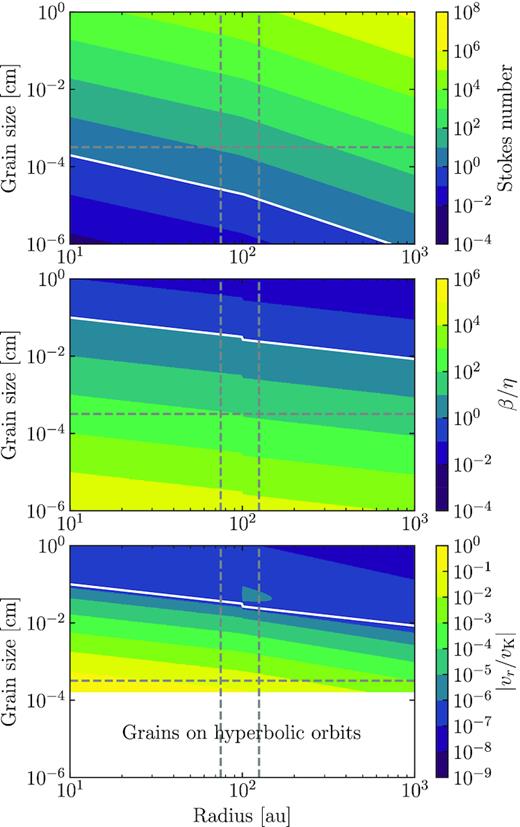
$Effect of gas on dust as a function of grain size and stellar distance assuming a steady state surface density of gas when released at 100 au, reaching a local surface density of 10−6 M⊕ au−2. Top: Dimensionless stopping time of Stokes number in the subsonic regime. The white line represents a Stokes number of one. Middle: Ratio between the β (the radiation to gravitational force ratio) and η the ratio between the pressure gradient force and gravitational force. If larger than 1, then grains will be pushed outwards and vice versa. Bottom: Modulus of the radial velocity of dust grains over the Keplerian velocity. In the three panels, the horizontal dashed line represents the blowout size for an A3V star and the vertical dashed lines represent the inner and outer edge of a belt at 100 au with a fractional width of 0.5.$

Figure 11.

Effect of gas on dust as a function of grain size and stellar distance assuming a steady state surface density of gas when released at 100 au, reaching a local surface density of 10⁻⁶ M_⊕ au⁻². Top: Dimensionless stopping time of Stokes number in the subsonic regime. The white line represents a Stokes number of one. Middle: Ratio between the β (the radiation to gravitational force ratio) and η the ratio between the pressure gradient force and gravitational force. If larger than 1, then grains will be pushed outwards and vice versa. Bottom: Modulus of the radial velocity of dust grains over the Keplerian velocity. In the three panels, the horizontal dashed line represents the blowout size for an A3V star and the vertical dashed lines represent the inner and outer edge of a belt at 100 au with a fractional width of 0.5.

Open in new tab Download slide

Even though grains above the blowout size have larger Stokes numbers, they could still systematically migrate in or out due to a difference in their orbital speed. Ignoring Poynting–Robertson drag (PR drag), the azimuthal velocity of a dust grain on a circular orbit is

$$\begin{eqnarray*} v_{\phi }=v_\mathrm{K}(1-\beta)^{1/2}, \end{eqnarray*}$$

(25)

where β is the ratio between the radiation and gravitational forces (Burns et al. 1979), thus small grains in circular orbits will have sub-Keplerian speeds. Similarly, because of pressure support gas will also orbit at a sub-Keplerian speed that is

$$\begin{eqnarray*} v_\mathrm{g} &=& v_\mathrm{K}(1-\eta)^{1/2},\\ \eta &=& - \frac{1}{r\Omega _\mathrm{K}^2 \rho _\mathrm{g}}\frac{dP_\mathrm{g}}{dr}, \end{eqnarray*}$$

(26),(27)

where ρ_g and P_g are the gas density and pressure, respectively, and η the ratio between the pressure gradient force and gravitational force. If β > η, dust grains will orbit slower than the gas, and thus gas drag will increase their angular momentum producing an outward migration (Takeuchi & Artymowicz 2001). In the middle plot of Fig. 11, we show the ratio β/η for different grain sizes at different radii. We calculate β assuming blackbody grains with an internal density of 2.7 g cm⁻³ and η according to blackbody temperatures and the analytic expression for the gas surface density profile. We find that grains below 1 mm have β > η and thus will experience outward migration, while larger grains will tend to migrate inwards. This will only happen if the time-scales are shorter or comparable to the collisional lifetime of these grains. Using equation (26) in Takeuchi & Artymowicz (2001), which assumes circular orbits, we compute the radial velocity of grains under the influence of gas and PR drag too (Fig. 11 bottom panel). We find that for small µm-sized grains their radial speed could be a few per cent of the Keplerian speed, and thus could exit the planetesimal belt within a few orbits.

Small grains will only migrate out of the belt efficiently if they can do so on a time-scale shorter than their collisional time-scale. In Fig. 12, we compare the time-scale at which a small grain at the bottom of the collisional cascade on a circular orbit would exit the belt, assuming a disc width of 50 au, with their collisional time-scale as a function of the disc fractional luminosity. For this, we use equations (B5) and (B6) in Matrà et al. (2017b) to calculate the mass-loss rate and collisional time-scales. We also assume a CO mass fraction of 0.1 inside planetesimals, which sets the gas release rate and thus the gas surface density which will affect the dust. We find that for α = 0.1 (blue line) and fractional luminosities larger than 10⁻³, grains can exit the belt on time-scales shorter than their collisional lifetime (blue line is below the dashed black line). For smaller f_IR drift time-scales due to gas drag become too long, and actually, for f_IR < 6 × 10⁻⁵ PR drag dominates as a drag force (see the blue line converging to the black dotted line). Nevertheless, PR drag time-scales will be longer than collisional time-scales for f_IR > 4 × 10⁻⁶, which is at the limit of detectability with current instrumentation (see Wyatt 2005, for a detailed discussion on PR drag). For smaller α’s, gas drag could become important even in less-massive planetesimal discs since gas can accumulate for longer and thus build larger gas surface densities. For α = 10⁻³, small dust in discs with f_IR > 2 × 10⁻⁵ could efficiently migrate outwards with the fastest drift achieved with f_IR ∼ 10⁻³, which is when the Stokes number for grains with β = 0.5 is equal to 1. Therefore, we conclude that outward migration of small dust grains due to gas drag in exocometary gaseous discs could be an efficient process, increasing the cross-sectional area of disc haloes (e.g. HD32297, Schneider et al. 2005; Bhowmik et al. 2019).

Figure 12.

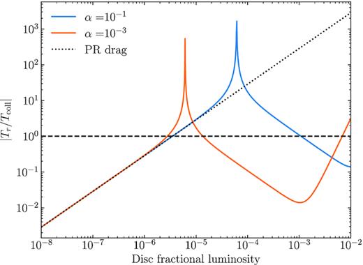
Radial migration time-scale over collisional time-scales for dust grains at the bottom of the collisional cascade. The blue and orange lines represent a case with an α viscosity value of 10⁻³ and 0.1, respectively. The black dotted line represents a case when neglecting gas drag and considering PR drag only.

Open in new tab Download slide

Based on the derived Stokes numbers, we find that photoelectric instability (Lyra & Kuchner 2013; Richert, Lyra & Kuchner 2018) should not play a major role affecting the distribution of gas and dust. This is because the Stokes numbers are significantly larger than unity for all grains sizes above the blowout size, and the dust-to-gas ratio is expected to be much lower than unity when considering only grains smaller than 10 µm as in Richert et al. (2018, see their fig. 2).

Finally, it is possible that the overall gas surface densities are higher than assumed here if other volatiles (e.g. water) are being released as well. Assuming a water ice fraction of 0.5 in planetesimals, the gas surface densities would be a factor 5 larger than assumed. Therefore, dust grains close to the blow-out size would have lower Stokes numbers in the range 1–10 (as suggested in Bhowmik et al. 2019), and migrate outwards even faster. Note that the smaller Stokes number could be enough to trigger the photoelectric instability, although the higher gas surface density would also decrease the dust-to-gas ratio. Detailed simulations are necessary to assess whether this instability could act on time-scales shorter than the age of these systems with these dust-to-gas ratios and Stokes numbers.

5.7 Mass-loss rate inferred from the SED

In this paper, we have shown that overall CO gas observations around A stars can be explained with our population synthesis model presented in Section 3. Nevertheless, this is not entirely satisfactory since our model has three main free parameters to fit one main observable, the observed CO gas mass. Moreover, these parameters (the viscosity, the fraction of CO in planetesimals, and the maximum planetesimal size or initial median disc mass) are degenerated. In Sections 5.2.1 and 5.2.2, we discuss how the first two could be constrained through independent methods and thus break degeneracies. The maximum planetesimal size is however unconstrained by the collisional model used here. Namely, given a disc radius and fractional luminosity, the total disc mass and mass-loss rate are unconstrained. Matrà et al. (2017b) showed however that the mass-loss rate at the bottom of the collisional cascade can indeed be estimated analytically based on the disc cross-sectional area and minimum grain size. The reason for this is that the lifetime or collisional rate of the smallest grains (near the blowout size) is dominated by grains of similar size which is not the case at the top of the size distribution. This slight but significant difference is not accounted for in the collisional model used here which assumes a single power-law size distribution.

In Fig. 13, we compare the mass-loss rate used in our model (Section 3) versus the mass-loss rate that would be inferred from the model fractional luminosity using equation (B6) in Matrà et al. (2017b). We find that for the chosen parameters (e = 0.001, D_c = 0.02 km, |${Q_\mathrm{D}^{\star }}=1.6$| J kg⁻¹, and M_mid = 0.5 M_⊕) the mass-loss rate in our model roughly agrees with the one calculated considering the bottom of the collisional cascade (⁠|$\dot{M}_{D_\mathrm{min}}$|⁠), except for belts with radius smaller than ∼50 au. The dependence on belt radius is due to both analytic expressions having a different dependence on r_belt. The belt radius sets the Keplerian and relative velocities, which are important for determining the minimum planetesimal size that disrupt the planetesimals at the top of the size distribution, whereas at the bottom of the size distribution that size is simply set by the blowout size. In order to reconcile the mass-loss rate from small grains and the largest planetesimals, more detailed modelling is necessary taking into account, for example, the size dependent planetesimal strength and wavy patterns in the size distribution (Krivov et al. 2006; Thébault & Augereau 2007).

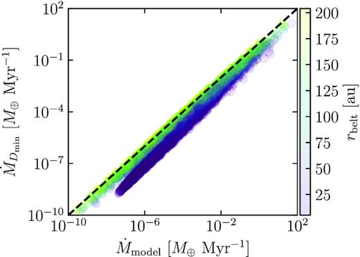
$Mass-loss rate used in our modelling based on planetesimal parameters and total mass (x-axis) versus mass-loss rate derived from our model fractional luminosity as in Matrà et al. (2017b, y-axis). Each circle corresponds to a different simulation presented in Section 3.1, and are colour coded according to their belt radius, with purple circles representing small belts and yellow circles large belts. The dashed line represents the y = x curve, i.e. points along the dashed line have consistent mass-loss rates.$

Figure 13.

Mass-loss rate used in our modelling based on planetesimal parameters and total mass (x-axis) versus mass-loss rate derived from our model fractional luminosity as in Matrà et al. (2017b, y-axis). Each circle corresponds to a different simulation presented in Section 3.1, and are colour coded according to their belt radius, with purple circles representing small belts and yellow circles large belts. The dashed line represents the y = x curve, i.e. points along the dashed line have consistent mass-loss rates.

Open in new tab Download slide

5.8 Hydrodynamic limit

Finally, here we discuss whether it is reasonable to treat the evolution of exocometary gaseous discs with the standard viscous evolution equations used here. While these equations are normally valid for the evolution of protoplanetary discs, the gas densities in the exocometary gas context can be much lower and thus we may approach the limit at which these equations are valid. To check this, we compare the disc scale height (H = c_s/Ω_K) with the mean free path in the gas, l (see Kral et al. 2016, for a specific discussion related to β Pic’s gaseous disc). We find that at 100 au, the mean free path of gas (not ionized) in the mid-plane will be smaller than H as long as the gas surface density is larger than ∼10⁻⁹ M_⊕ au⁻². If the gas is highly ionized as expected for low-density discs, the mean free path will be orders of magnitude smaller due to the large cross-section of ionized species, and therefore we estimate that for surface densities larger than ∼10⁻¹⁷ M_⊕ au⁻² our treatment is valid. This surface density is much lower than the typical gas surface densities of shielded discs (≳10⁻⁷ M_⊕ au⁻²) and the unshielded gas discs detected around A stars (M_gas > 10⁻⁵ M_⊕). Only for the lower tail of the population distribution of surface densities around A stars (see Fig. 4), the mean free path of molecules and atoms could be comparable or larger than H and thus the evolution of those discs with extreme low gas masses must be taken with caution. Note that this critical surface density is not very sensitive to the choice of H since l is proportional to H.

6 CONCLUSIONS

In this paper, we have presented a new numerical model to explain the presence of gas found around nearby young stars with debris discs, with an emphasis on A stars. This gas originates in the interior of planetesimals, and mutual collisions release both dust and gas. Our model (Section 2) solves for the viscous evolution of the gas (CO, carbon, and oxygen) in 1D as it is released by planetesimals (in the form of CO), taking into account the CO photodissociation, self-shielding, and shielding by neutral carbon. Our model has one significant addition compared to previous work, it takes into account the time dependent gas release rate due to the disc collisional evolution.

With this model, we found that the present gas mass of a disc is highly dependant on the assumed initial disc mass in the form of planetesimals. A system with a constant gas input rate can have a gas mass orders of magnitude lower compared to a system that started with a higher mass and collisionally evolved to an equal planetesimal disc mass. Because of the nature of collisional evolution of planetesimal discs, dust levels do not depend strongly on the initial disc mass and therefore it is a degenerate problem to try to infer the initial disc mass from dust levels. This means that while a disc might contain low quantities of dust in a collisionally evolved disc, it might have a massive gas disc due to a large initial disc mass. These considerations must be taken into account when analysing gas observations and comparing it with dust levels. However, if CO is unshielded, its short lifetime (∼120 yr) means that its mass will be set by the present mass-loss rate. Conversely, atomic carbon has a longer lifetime as it will viscously evolve on longer time-scales which will depend on the kinematic viscosity.

We used this new numerical code to produce the first population synthesis model for exocometary gas around A stars. Population synthesis studies are ideal to deal with degenerated problems and provide constraints on population properties rather than individual systems. Informed by previous studies that fit the dust evolution, we generated samples of 10⁴ stars hosting planetesimal discs with random radius, mass, and stellar properties. We evolved these systems up to a random age between 3–100 Myr and compare the final distribution to the observed distribution by applying the same selection filters to our model population. We found that our model can reproduce the distribution of CO masses well when viscosities are high (α ≈ 0.1), even producing a bimodal distribution with a large population of unshielded CO discs and a small fraction of shielded ones. The shielded population is nevertheless common in our models among systems with bright debris discs, which explains why shielded discs are common among the sample of 17 A stars with bright and cold debris discs. The high-α value implies that gas needs to be lost on time-scales of ∼1–10 Myr. Otherwise, carbon readily accumulates shielding CO and producing a large population of shielded and massive CO discs, even around systems with low planetesimal disc masses, which is inconsistent with observations.

Although, we focused on A stars, we also tested our model against observations of FGK stars. While massive and shielded CO gas discs are found around A stars, observations of FGK stars have showed that these have low CO gas masses, with only a few detections. Using our model, we showed that this is consistent with the collisional evolution studies of discs around FGK stars compared to A stars. Their lower initial disc masses means that gas release rates are lower. Our model quantitatively shows that massive CO gas discs should be very rare around FGK stars if they have similar viscosity levels compared to A stars.

An important test of viscous evolution models of gas in debris discs, is whether gas is observed to extend inwards and accrete on to the star. In Section 5, we discussed recent observations of neutral carbon around a few systems which seem to indicate that carbon has not spread inwards forming an accretion disc as expected in a viscous evolution scenario. This might suggest that either gas release started recently or is lost through another mechanism, e.g. radiation pressure. Nevertheless, our modelling constrains the gas loss time-scale to be ∼1–10 Myr (viscous time-scale), which could provide insights into alternative mass-loss mechanisms. More resolved observations of carbon are needed to conclude.

A potential explanation for the observed cavities in the distribution of carbon could be the presence of planets. A planet orbiting the system interior to the planetesimal belt could block the inward flow of gas if more massive that ≳50 M_⊕, accreting most of the exocometary gas flowing in. In this scenario, the gas distribution and dynamics could provide constraints on the mass and location of planets at tens of au and interior to massive planetesimal belts.

Finally, we also discussed if gas could affect the dynamics of dust grains. We found that dust should not be heavily affected by gas drag. Only small sub-µm grains that are unbound due to radiation pressure could feel a strong gas drag that could slow their unbound trajectories. However, we find that the predicted gas densities could be high enough to make µm-sized grains to effectively migrate out on time-scales comparable to their collisional time-scales.

ACKNOWLEDGEMENTS

We thank Richard Booth for valuable input and advice in setting up the numerical code to solve for the viscous evolution of gas considering multiple species. We also thank the anonymous referee for a constructive and thorough review. TH acknowledges support from the European Research Council under the Horizon 2020 Framework Program via the ERC Advanced Grant Origins 83 24 28. LM acknowledges support from the Smithsonian Institution as a Submillimeter Array (SMA) Fellow.

Footnotes

1

Note that there is a typo in Wyatt et al. (2007b)’s equation as it should be in years rather than Myr

2

To increase the number of points of this filtered sample, we simulated 8000 extra systems with the same initial random distribution, but that passed the Moór et al. selection criteria.

3

Note that Δv_line is defined as |$\sigma _\mathrm{line}/\sqrt{2}$|⁠, with σ_line being the standard deviation of the line profile.

4

Calculated at 40 au using their best-fitting parameters.

5

Using the subsonic stopping time.

REFERENCES

Bath

G. T.

,

Pringle

J. E.

,

1981

,

MNRAS

,

194

,

967

10.1093/mnras/194.4.967

Crossref

Search ADS

Benz

W.

,

Asphaug

E.

,

1999

,

Icarus

,

142

,

5

10.1006/icar.1999.6204

Crossref

Search ADS

Beust

H.

,

Morbidelli

A.

,

1996

,

Icarus

,

120

,

358

10.1006/icar.1996.0056

Crossref

Search ADS

Beust

H.

,

Vidal-Madjar

A.

,

Ferlet

R.

,

Lagrange-Henri

A. M.

,

1990

,

A&A

,

236

,

202

Bhowmik

T.

et al. .,

2019

,

A&A

,

630

,

A85

Crossref

Search ADS

Booth

M.

et al. .,

2013

,

MNRAS

,

428

,

1263

10.1093/mnras/sts117

Crossref

Search ADS

Booth

R. A.

,

Clarke

C. J.

,

Madhusudhan

N.

,

Ilee

J. D.

,

2017

,

MNRAS

,

469

,

3994

10.1093/mnras/stx1103

Crossref

Search ADS

Booth

M.

et al. .,

2019

,

MNRAS

,

482

,

3443

10.1093/mnras/sty2993

Crossref

Search ADS

Bouret

J. C.

,

Deleuil

M.

,

Lanz

T.

,

Roberge

A.

,

Lecavelier des Etangs

A.

,

Vidal-Madjar

A.

,

2002

,

A&A

,

390

,

1049

10.1051/0004-6361:20020741

Crossref

Search ADS

Bovy

J.

,

2017

,

MNRAS

,

470

,

1360

10.1093/mnras/stx1277

Crossref

Search ADS

Bowler

B. P.

,

Nielsen

E. L.

,

2018

, in

Deeg

H.

,

Belmonte

J.

, eds,

Handbook of Exoplanets: Occurrence Rates from Direct Imaging Surveys

.

Springer

,

Cham

, p.

155

Google Scholar

Google Preview

OpenURL Placeholder Text

WorldCat

Burns

J. A.

,

Lamy

P. L.

,

Soter

S.

,

1979

,

Icarus

,

40

,

1

10.1016/0019-1035(79)90050-2

Crossref

Search ADS

Cataldi

G.

et al. .,

2014

,

A&A

,

563

,

A66

10.1051/0004-6361/201323126

Crossref

Search ADS

Cataldi

G.

et al. .,

2018

,

ApJ

,

861

,

72

10.3847/1538-4357/aac5f3

Crossref

Search ADS

Cataldi

G.

et al. .,

2019

,

preprint (arXiv:1904.07215)

Cavallius

M.

,

Cataldi

G.

,

Brandeker

A.

,

Olofsson

G.

,

Larsson

B.

,

Liseau

R.

,

2019

,

A&A

,

628

,

A127

Crossref

Search ADS

Crida

A.

,

Morbidelli

A.

,

Masset

F.

,

2006

,

Icarus

,

181

,

587

10.1016/j.icarus.2005.10.007

Crossref

Search ADS

Deleuil

M.

et al. .,

2001

,

ApJ

,

557

,

L67

10.1086/323005

Crossref

Search ADS

Dent

W. R. F.

et al. .,

2014

,

Science

,

343

,

1490

10.1126/science.1248726

Crossref

Search ADS

PubMed

Dominik

C.

,

Decin

G.

,

2003

,

ApJ

,

598

,

626

10.1086/379169

Crossref

Search ADS

Draine

B. T.

,

1978

,

ApJS

,

36

,

595

10.1086/190513

Crossref

Search ADS

Ferlet

R.

,

Vidal-Madjar

A.

,

Hobbs

L. M.

,

1987

,

A&A

,

185

,

267

Fernández

R.

,

Brandeker

A.

,

Wu

Y.

,

2006

,

ApJ

,

643

,

509

10.1086/500788

Crossref

Search ADS

Flaherty

K. M.

et al. .,

2016

,

ApJ

,

818

,

97

10.3847/0004-637X/818/1/97

Crossref

Search ADS

Greaves

J. S.

et al. .,

2016

,

MNRAS

,

461

,

3910

10.1093/mnras/stw1569

Crossref

Search ADS

Grigorieva

A.

,

Thébault

P.

,

Artymowicz

P.

,

Brandeker

A.

,

2007

,

A&A

,

475

,

755

10.1051/0004-6361:20077686

Crossref

Search ADS

Hales

A. S.

,

Gorti

U.

,

Carpenter

J. M.

,

Hughes

M.

,

Flaherty

K.

,

2019

,

ApJ

,

878

,

113

10.3847/1538-4357/ab211e

Crossref

Search ADS

Higuchi

A. E.

et al. .,

2017

,

ApJ

,

839

,

L14

10.3847/2041-8213/aa67f4

Crossref

Search ADS

Higuchi

A. E.

et al. .,

2019

,

ApJ

,

883

,

180

Crossref

Search ADS

Hudson

R. D.

,

1971

,

Rev. Geophys. Space Phys.

,

9

,

305

10.1029/RG009i002p00305

Crossref

Search ADS

Hughes

A. M.

,

Wilner

D. J.

,

Andrews

S. M.

,

Qi

C.

,

Hogerheijde

M. R.

,

2011

,

ApJ

,

727

,

85

10.1088/0004-637X/727/2/85

Crossref

Search ADS

Hughes

A. M.

et al. .,

2017

,

ApJ

,

839

,

86

10.3847/1538-4357/aa6b04

Crossref

Search ADS

Iglesias

D.

et al. .,

2018

,

MNRAS

,

480

,

488

10.1093/mnras/sty1724

Crossref

Search ADS

Kains

N.

,

Wyatt

M. C.

,

Greaves

J. S.

,

2011

,

MNRAS

,

414

,

2486

10.1111/j.1365-2966.2011.18566.x

Crossref

Search ADS

Kennedy

G. M.

,

Marino

S.

,

Matrà

L.

,

Panić

O.

,

Wilner

D.

,

Wyatt

M. C.

,

Yelverton

B.

,

2018

,

MNRAS

,

475

,

4924

10.1093/mnras/sty135

Crossref

Search ADS

Kiefer

F.

,

Lecavelier des Etangs

A.

,

Boissier

J.

,

Vidal-Madjar

A.

,

Beust

H.

,

Lagrange

A.-M.

,

Hébrard

G.

,

Ferlet

R.

,

2014

,

Nature

,

514

,

462

Kóspál

Á.

et al. .,

2013

,

ApJ

,

776

,

77

Crossref

Search ADS

Kral

Q.

,

Latter

H.

,

2016

,

MNRAS

,

461

,

1614

10.1093/mnras/stw1429

Crossref

Search ADS

Kral

Q.

,

Thébault

P.

,

Charnoz

S.

,

2013

,

A&A

,

558

,

A121

10.1051/0004-6361/201321398

Crossref

Search ADS

Kral

Q.

,

Wyatt

M.

,

Carswell

R. F.

,

Pringle

J. E.

,

Matrà

L.

,

Juhász

A.

,

2016

,

MNRAS

,

461

,

845

10.1093/mnras/stw1361

Crossref

Search ADS

Kral

Q.

,

Matrà

L.

,

Wyatt

M. C.

,

Kennedy

G. M.

,

2017

,

MNRAS

,

469

,

521

10.1093/mnras/stx730

Crossref

Search ADS

Kral

Q.

,

Marino

S.

,

Wyatt

M. C.

,

Kama

M.

,

Matrà

L.

,

2019

,

MNRAS

,

489

,

3670

10.1093/mnras/sty2923

Crossref

Krivov

A. V.

,

Löhne

T.

,

Sremčević

M.

,

2006

,

A&A

,

455

,

509

10.1051/0004-6361:20064907

Crossref

Search ADS

Krivov

A. V.

,

Ide

A.

,

Löhne

T.

,

Johansen

A.

,

Blum

J.

,

2018

,

MNRAS

,

474

,

2564

10.1093/mnras/stx2932

Crossref

Search ADS

Kuiper

R.

,

Hosokawa

T.

,

2018

,

A&A

,

616

,

A101

10.1051/0004-6361/201832638

Crossref

Search ADS

Lecavelier Des Etangs

A.

,

Vidal-Madjar

A.

,

Ferlet

R.

,

1998

,

A&A

,

339

,

477

Lenz

D. D.

,

Ayres

T. R.

,

1992

,

PASP

,

104

,

1104

10.1086/133096

Crossref

Search ADS

Lieman-Sifry

J.

,

Hughes

A. M.

,

Carpenter

J. M.

,

Gorti

U.

,

Hales

A.

,

Flaherty

K. M.

,

2016

,

ApJ

,

828

,

25

10.3847/0004-637X/828/1/25

Crossref

Search ADS

Löhne

T.

,

Krivov

A. V.

,

Rodmann

J.

,

2008

,

ApJ

,

673

,

1123

10.1086/524840

Crossref

Search ADS

Lubow

S. H.

,

D’Angelo

G.

,

2006

,

ApJ

,

641

,

526

Crossref

Search ADS

Lubow

S. H.

,

Seibert

M.

,

Artymowicz

P.

,

1999

,

ApJ

,

526

,

1001

10.1086/308045

Crossref

Search ADS

Lynden-Bell

D.

,

Pringle

J. E.

,

1974

,

MNRAS

,

168

,

603

10.1093/mnras/168.3.603

Crossref

Search ADS

Lyra

W.

,

Kuchner

M.

,

2013

,

Nature

,

499

,

184

MacGregor

M. A.

et al. .,

2018

,

ApJ

,

869

,

75

10.3847/1538-4357/aaec71

Crossref

Search ADS

Machida

M. N.

,

Kokubo

E.

,

Inutsuka

S.-I.

,

Matsumoto

T.

,

2010

,

MNRAS

,

405

,

1227

10.1111/j.1365-2966.2010.16527.x

Crossref

Marino

S.

et al. .,

2016

,

MNRAS

,

460

,

2933

10.1093/mnras/stw1216

Crossref

Search ADS

Marino

S.

et al. .,

2017

,

MNRAS

,

465

,

2595

10.1093/mnras/stw2867

Crossref

Search ADS

Marino

S.

et al. .,

2018

,

MNRAS

,

479

,

5423

10.1093/mnras/sty1790

Crossref

Search ADS

Marino

S.

,

Yelverton

B.

,

Booth

M.

,

Faramaz

V.

,

Kennedy

G. M.

,

Matrà

L.

,

Wyatt

M. C.

,

2019

,

MNRAS

,

484

,

1257

10.1093/mnras/stz049

Crossref

Search ADS

Matrà

L.

et al. .,

2017a

,

MNRAS

,

464

,

1415

10.1093/mnras/stw2415

Crossref

Search ADS

Matrà

L.

et al. .,

2017b

,

ApJ

,

842

,

9

10.3847/1538-4357/aa71b4

Crossref

Search ADS

Matrà

L.

,

Wilner

D. J.

,

Öberg

K. I.

,

Andrews

S. M.

,

Loomis

R. A.

,

Wyatt

M. C.

,

Dent

W. R. F.

,

2018a

,

ApJ

,

853

,

147

10.3847/1538-4357/aaa42a

Crossref

Search ADS

Matrà

L.

,

Marino

S.

,

Kennedy

G. M.

,

Wyatt

M. C.

,

Öberg

K. I.

,

Wilner

D. J.

,

2018b

,

ApJ

,

859

,

72

10.3847/1538-4357/aabcc4

Crossref

Search ADS

Matrà

L.

,

Öberg

K. I.

,

Wilner

D. J.

,

Olofsson

J.

,

Bayo

A.

,

2019

,

AJ

,

157

,

117

10.3847/1538-3881/aaff5b

Crossref

Search ADS

Metzger

B. D.

,

Rafikov

R. R.

,

Bochkarev

K. V.

,

2012

,

MNRAS

,

423

,

505

10.1111/j.1365-2966.2012.20895.x

Crossref

Search ADS

Montgomery

S. L.

,

Welsh

B. Y.

,

2012

,

PASP

,

124

,

1042

10.1086/668293

Crossref

Search ADS

Moór

A.

et al. .,

2011

,

ApJ

,

740

,

L7

10.1088/2041-8205/740/1/L7

Crossref

Search ADS

Moór

A.

et al. .,

2015

,

ApJ

,

814

,

42

10.1088/0004-637X/814/1/42

Crossref

Search ADS

Moór

A.

et al. .,

2017

,

ApJ

,

849

,

123

10.3847/1538-4357/aa8e4e

Crossref

Search ADS

Moór

A.

et al. .,

2019

,

ApJ

,

884

,

108

Crossref

Search ADS

Mordasini

C.

,

Alibert

Y.

,

Benz

W.

,

2009

,

A&A

,

501

,

1139

10.1051/0004-6361/200810301

Crossref

Search ADS

Mumma

M. J.

,

Charnley

S. B.

,

2011

,

ARA&A

,

49

,

471

10.1146/annurev-astro-081309-130811

Crossref

Search ADS

Mustill

A. J.

,

Wyatt

M. C.

,

2009

,

MNRAS

,

399

,

1403

10.1111/j.1365-2966.2009.15360.x

Crossref

Search ADS

Olofsson

J.

et al. .,

2016

,

A&A

,

591

,

A108

10.1051/0004-6361/201628196

Crossref

Search ADS

Pawellek

N.

,

Krivov

A. V.

,

2015

,

MNRAS

,

454

,

3207

10.1093/mnras/stv2142

Crossref

Search ADS

Pawellek

N.

,

Krivov

A. V.

,

Marshall

J. P.

,

Montesinos

B.

,

Ábrahám

P.

,

Moór

A.

,

Bryden

G.

,

Eiroa

C.

,

2014

,

ApJ

,

792

,

65

10.1088/0004-637X/792/1/65

Crossref

Search ADS

Rebollido

I.

et al. .,

2018

,

A&A

,

614

,

A3

10.1051/0004-6361/201732329

Crossref

Search ADS

Richert

A. J. W.

,

Lyra

W.

,

Kuchner

M. J.

,

2018

,

ApJ

,

856

,

41

10.3847/1538-4357/aaadaa

Crossref

Search ADS

Rieke

G. H.

et al. .,

2005

,

ApJ

,

620

,

1010

10.1086/426937

Crossref

Search ADS

Riviere-Marichalar

P.

et al. .,

2012

,

A&A

,

546

,

L8

10.1051/0004-6361/201219745

Crossref

Search ADS

Roberge

A.

et al. .,

2013

,

ApJ

,

771

,

69

10.1088/0004-637X/771/1/69

Crossref

Search ADS

Rollins

R. P.

,

Rawlings

J. M. C.

,

2012

,

MNRAS

,

427

,

2328

10.1111/j.1365-2966.2012.22121.x

Crossref

Search ADS

Schneider

G.

,

Silverstone

M. D.

,

Hines

D. C.

,

2005

,

ApJ

,

629

,

L117

10.1086/452631

Crossref

Search ADS

Sepulveda

A. G.

et al. .,

2019

,

ApJ

,

881

,

84

Crossref

Search ADS

Sibthorpe

B.

,

Kennedy

G. M.

,

Wyatt

M. C.

,

Lestrade

J. F.

,

Greaves

J. S.

,

Matthews

B. C.

,

Duchêne

G.

,

2018

,

MNRAS

,

475

,

3046

10.1093/mnras/stx3188

Crossref

Search ADS

Slettebak

A.

,

1975

,

ApJ

,

197

,

137

10.1086/153493

Crossref

Search ADS

Stevenson

D. J.

,

1990

,

ApJ

,

348

,

730

10.1086/168282

Crossref

Search ADS

Su

K. Y. L.

et al. .,

2006

,

ApJ

,

653

,

675

10.1086/508649

Crossref

Search ADS

Takeuchi

T.

,

Artymowicz

P.

,

2001

,

ApJ

,

557

,

990

10.1086/322252

Crossref

Search ADS

Tazaki

R.

,

Nomura

H.

,

2015

,

ApJ

,

799

,

119

10.1088/0004-637X/799/2/119

Crossref

Search ADS

Teague

R.

,

Bae

J.

,

Bergin

E. A.

,

Birnstiel

T.

,

Foreman-Mackey

D.

,

2018

,

ApJ

,

860

,

L12

10.3847/2041-8213/aac6d7

Crossref

Search ADS

Thébault

P.

,

Augereau

J.-C.

,

2007

,

A&A

,

472

,

169

10.1051/0004-6361:20077709

Crossref

Search ADS

Turner

N. J.

,

Willacy

K.

,

Bryden

G.

,

Yorke

H. W.

,

2006

,

ApJ

,

639

,

1218

10.1086/499486

Crossref

Search ADS

van Dishoeck

E. F.

,

Black

J. H.

,

1988

,

ApJ

,

334

,

771

10.1086/166877

Crossref

Search ADS

van Dishoeck

E. F.

,

Jonkheid

B.

,

van Hemert

M. C.

,

2006

,

Faraday Discuss.

,

133

,

231

Visser

R.

,

van Dishoeck

E. F.

,

Black

J. H.

,

2009

,

A&A

,

503

,

323

10.1051/0004-6361/200912129

Crossref

Search ADS

Welsh

B. Y.

,

Montgomery

S. L.

,

2018

,

MNRAS

,

474

,

1515

10.1093/mnras/stx2800

Crossref

Search ADS

Wyatt

M. C.

,

2005

,

A&A

,

433

,

1007

10.1051/0004-6361:20042073

Crossref

Search ADS

Wyatt

M. C.

,

2008

,

ARA&A

,

46

,

339

10.1146/annurev.astro.45.051806.110525

Crossref

Search ADS

Wyatt

M. C.

,

Dent

W. R. F.

,

2002

,

MNRAS

,

334

,

589

10.1046/j.1365-8711.2002.05533.x

Crossref

Search ADS

Wyatt

M. C.

,

Smith

R.

,

Greaves

J. S.

,

Beichman

C. A.

,

Bryden

G.

,

Lisse

C. M.

,

2007a

,

ApJ

,

658

,

569

10.1086/510999

Crossref

Search ADS

Wyatt

M. C.

,

Smith

R.

,

Su

K. Y. L.

,

Rieke

G. H.

,

Greaves

J. S.

,

Beichman

C. A.

,

Bryden

G.

,

2007b

,

ApJ

,

663

,

365

10.1086/518404

Crossref

Search ADS

Zuckerman

B.

,

Song

I.

,

2012

,

ApJ

,

758

,

77

10.1088/0004-637X/758/2/77

Crossref

Search ADS

Zuckerman

B.

,

Forveille

T.

,

Kastner

J. H.

,

1995

,

Nature

,

373

,

494

Öberg

K. I.

,

Murray-Clay

R.

,

Bergin

E. A.

,

2011

,

ApJ

,

743

,

L16

10.1088/2041-8205/743/1/L16

Crossref

Search ADS

APPENDIX A: GAS OBSERVATIONS USED IN THIS WORK

In Tables A1 and A2, we show the properties of each of the observed systems that were used to compare to our population synthesis model. Table A1 only shows A stars with ages between 10 and 50 Myr and debris discs that have fractional luminosities between 5 × 10⁻⁴–0.01 and dust temperatures below 140 K. Table A2 shows a similar filtered sample, but without an age restriction. Note that there has not been a complete survey for FGK stars with a selection criteria similar to Moór et al. (2017), and thus Table A2 is likely incomplete.

Table A1.

Open in new tab

Properties of A stars with high fractional luminosity discs (5 × 10⁻⁴–0.01), ages ranging between 10 and 50 Myr and dust temperatures lower than 140 K. The upper limits correspond to 99.7 per cent confidence levels.

Name	Age (Myr)	L_⋆ (L_⊙)	f_IR	r_belt (au)	M_CO (M_⊕)	M_C (M_⊕)	Ref.
β Pic	23	8.7	2.6 × 10⁻³	105	2.8 × 10⁻⁵	1.0 × 10⁻³	1, 2
49 Ceti	40	16	7.2 × 10⁻⁴	96	1.4 × 10⁻⁴	4.0 × 10⁻³	3, 4
HD 21997	45	9.9	5.6 × 10⁻⁴	106	6 × 10⁻²	–	5
HD 32297	30	8.2	5.5 × 10⁻³	100	1.3 × 10⁻³	3.5 × 10⁻³	6, 7, 8, 9
HD 95086	15	6.1	1.4 × 10⁻³	204	4.3 × 10⁻⁶	–	10
HD 98363	15	11	1.3 × 10⁻³	32^⋆	<9.5 × 10⁻⁶	–	11, 12
HD 109832	15	5.3	5.4 × 10⁻⁴	25^⋆	<7. × 10⁻⁶	–	11, 12
HD 110058	15	5.9	1.4 × 10⁻³	50	2.1 × 10⁻⁵	–	7, 11, 13
HD 121191	16	7.2	4.5 × 10⁻³	26^⋆	2.7 × 10⁻³	–	11
HD 121617	16	17	4.9 × 10⁻³	83	1.8 × 10⁻²	–	11
HD 131488	16	13	2.2 × 10⁻³	84	8.9 × 10⁻²	–	11
HD 131835	16	11	2.2 × 10⁻³	90	4. × 10⁻²	3.3 × 10⁻³	13, 14, 15, 16
HD 138813	10	17	6. × 10⁻⁴	105	7.4 × 10⁻⁴	–	11, 13, 16
HD 143675	16	8.9	6.9 × 10⁻⁴	28^⋆	<1.7 × 10⁻⁵	–	11, 12
HD 145880	16	19	1.7 × 10⁻³	70^⋆	<2. × 10⁻⁵	–	11, 12
HD 156623	16	13	3.3 × 10⁻³	94	2.5 × 10⁻³	–	13, 16
HR 4796	10	26.	4.8 × 10⁻³	79	<3.7 × 10⁻⁶	–	19

Name	Age (Myr)	L_⋆ (L_⊙)	f_IR	r_belt (au)	M_CO (M_⊕)	M_C (M_⊕)	Ref.
β Pic	23	8.7	2.6 × 10⁻³	105	2.8 × 10⁻⁵	1.0 × 10⁻³	1, 2
49 Ceti	40	16	7.2 × 10⁻⁴	96	1.4 × 10⁻⁴	4.0 × 10⁻³	3, 4
HD 21997	45	9.9	5.6 × 10⁻⁴	106	6 × 10⁻²	–	5
HD 32297	30	8.2	5.5 × 10⁻³	100	1.3 × 10⁻³	3.5 × 10⁻³	6, 7, 8, 9
HD 95086	15	6.1	1.4 × 10⁻³	204	4.3 × 10⁻⁶	–	10
HD 98363	15	11	1.3 × 10⁻³	32^⋆	<9.5 × 10⁻⁶	–	11, 12
HD 109832	15	5.3	5.4 × 10⁻⁴	25^⋆	<7. × 10⁻⁶	–	11, 12
HD 110058	15	5.9	1.4 × 10⁻³	50	2.1 × 10⁻⁵	–	7, 11, 13
HD 121191	16	7.2	4.5 × 10⁻³	26^⋆	2.7 × 10⁻³	–	11
HD 121617	16	17	4.9 × 10⁻³	83	1.8 × 10⁻²	–	11
HD 131488	16	13	2.2 × 10⁻³	84	8.9 × 10⁻²	–	11
HD 131835	16	11	2.2 × 10⁻³	90	4. × 10⁻²	3.3 × 10⁻³	13, 14, 15, 16
HD 138813	10	17	6. × 10⁻⁴	105	7.4 × 10⁻⁴	–	11, 13, 16
HD 143675	16	8.9	6.9 × 10⁻⁴	28^⋆	<1.7 × 10⁻⁵	–	11, 12
HD 145880	16	19	1.7 × 10⁻³	70^⋆	<2. × 10⁻⁵	–	11, 12
HD 156623	16	13	3.3 × 10⁻³	94	2.5 × 10⁻³	–	13, 16
HR 4796	10	26.	4.8 × 10⁻³	79	<3.7 × 10⁻⁶	–	19

Note. References used in this table: (1): Matrà et al. (2017a); (2): Cataldi et al. (2018); (3): Hughes et al. (2017); (4): Higuchi et al. (2017); (5): Kóspál et al. (2013); (6): Greaves et al. (2016); (7): Kral et al. (2017); (8): MacGregor et al. (2018); (9): Cataldi et al. (2019); (10): Booth et al. (2019); (11): Moór et al. (2017); (12): upper limits derived in this work; (13): Lieman-Sifry et al. (2016); (14): Moór et al. (2015); (15): Kral et al. (2019); (16) Hales et al. (2019); and (17): Kennedy et al. (2018).

a

The belt radius is calculated as r_BB × 1.7.

Table A1.

Open in new tab

Properties of A stars with high fractional luminosity discs (5 × 10⁻⁴–0.01), ages ranging between 10 and 50 Myr and dust temperatures lower than 140 K. The upper limits correspond to 99.7 per cent confidence levels.

Name	Age (Myr)	L_⋆ (L_⊙)	f_IR	r_belt (au)	M_CO (M_⊕)	M_C (M_⊕)	Ref.
β Pic	23	8.7	2.6 × 10⁻³	105	2.8 × 10⁻⁵	1.0 × 10⁻³	1, 2
49 Ceti	40	16	7.2 × 10⁻⁴	96	1.4 × 10⁻⁴	4.0 × 10⁻³	3, 4
HD 21997	45	9.9	5.6 × 10⁻⁴	106	6 × 10⁻²	–	5
HD 32297	30	8.2	5.5 × 10⁻³	100	1.3 × 10⁻³	3.5 × 10⁻³	6, 7, 8, 9
HD 95086	15	6.1	1.4 × 10⁻³	204	4.3 × 10⁻⁶	–	10
HD 98363	15	11	1.3 × 10⁻³	32^⋆	<9.5 × 10⁻⁶	–	11, 12
HD 109832	15	5.3	5.4 × 10⁻⁴	25^⋆	<7. × 10⁻⁶	–	11, 12
HD 110058	15	5.9	1.4 × 10⁻³	50	2.1 × 10⁻⁵	–	7, 11, 13
HD 121191	16	7.2	4.5 × 10⁻³	26^⋆	2.7 × 10⁻³	–	11
HD 121617	16	17	4.9 × 10⁻³	83	1.8 × 10⁻²	–	11
HD 131488	16	13	2.2 × 10⁻³	84	8.9 × 10⁻²	–	11
HD 131835	16	11	2.2 × 10⁻³	90	4. × 10⁻²	3.3 × 10⁻³	13, 14, 15, 16
HD 138813	10	17	6. × 10⁻⁴	105	7.4 × 10⁻⁴	–	11, 13, 16
HD 143675	16	8.9	6.9 × 10⁻⁴	28^⋆	<1.7 × 10⁻⁵	–	11, 12
HD 145880	16	19	1.7 × 10⁻³	70^⋆	<2. × 10⁻⁵	–	11, 12
HD 156623	16	13	3.3 × 10⁻³	94	2.5 × 10⁻³	–	13, 16
HR 4796	10	26.	4.8 × 10⁻³	79	<3.7 × 10⁻⁶	–	19

Name	Age (Myr)	L_⋆ (L_⊙)	f_IR	r_belt (au)	M_CO (M_⊕)	M_C (M_⊕)	Ref.
β Pic	23	8.7	2.6 × 10⁻³	105	2.8 × 10⁻⁵	1.0 × 10⁻³	1, 2
49 Ceti	40	16	7.2 × 10⁻⁴	96	1.4 × 10⁻⁴	4.0 × 10⁻³	3, 4
HD 21997	45	9.9	5.6 × 10⁻⁴	106	6 × 10⁻²	–	5
HD 32297	30	8.2	5.5 × 10⁻³	100	1.3 × 10⁻³	3.5 × 10⁻³	6, 7, 8, 9
HD 95086	15	6.1	1.4 × 10⁻³	204	4.3 × 10⁻⁶	–	10
HD 98363	15	11	1.3 × 10⁻³	32^⋆	<9.5 × 10⁻⁶	–	11, 12
HD 109832	15	5.3	5.4 × 10⁻⁴	25^⋆	<7. × 10⁻⁶	–	11, 12
HD 110058	15	5.9	1.4 × 10⁻³	50	2.1 × 10⁻⁵	–	7, 11, 13
HD 121191	16	7.2	4.5 × 10⁻³	26^⋆	2.7 × 10⁻³	–	11
HD 121617	16	17	4.9 × 10⁻³	83	1.8 × 10⁻²	–	11
HD 131488	16	13	2.2 × 10⁻³	84	8.9 × 10⁻²	–	11
HD 131835	16	11	2.2 × 10⁻³	90	4. × 10⁻²	3.3 × 10⁻³	13, 14, 15, 16
HD 138813	10	17	6. × 10⁻⁴	105	7.4 × 10⁻⁴	–	11, 13, 16
HD 143675	16	8.9	6.9 × 10⁻⁴	28^⋆	<1.7 × 10⁻⁵	–	11, 12
HD 145880	16	19	1.7 × 10⁻³	70^⋆	<2. × 10⁻⁵	–	11, 12
HD 156623	16	13	3.3 × 10⁻³	94	2.5 × 10⁻³	–	13, 16
HR 4796	10	26.	4.8 × 10⁻³	79	<3.7 × 10⁻⁶	–	19

Note. References used in this table: (1): Matrà et al. (2017a); (2): Cataldi et al. (2018); (3): Hughes et al. (2017); (4): Higuchi et al. (2017); (5): Kóspál et al. (2013); (6): Greaves et al. (2016); (7): Kral et al. (2017); (8): MacGregor et al. (2018); (9): Cataldi et al. (2019); (10): Booth et al. (2019); (11): Moór et al. (2017); (12): upper limits derived in this work; (13): Lieman-Sifry et al. (2016); (14): Moór et al. (2015); (15): Kral et al. (2019); (16) Hales et al. (2019); and (17): Kennedy et al. (2018).

a

The belt radius is calculated as r_BB × 1.7.

Table A2.

Open in new tab

Properties of FGK stars with high fractional luminosity discs (5 × 10⁻⁴–0.01), with dust temperatures lower than 140 K and without age restrictions. The upper limits correspond to 99.7 per cent confidence levels.

Name	Age (Myr)	L_⋆ (L_⊙)	f_IR	r_belt (au)	M_CO (M_⊕)	Ref.
HD 61005	40	0.7	2.3 × 10⁻³	66	<6. × 10⁻⁶	1, 2, 3
HD 92945	100–300	0.37	6.6 × 10⁻⁴	87	<3 × 10⁻⁵	4
HD 107146	80–200	1.0	8.6 × 10⁻⁴	89	<5 × 10⁻⁶	5
HD 111520	15	3.0	1.1 × 10⁻³	96	<3 × 10⁻⁴	2, 3, 6
HD 145560	16	3.2	2.1 × 10⁻³	88	<2 × 10⁻⁴	2, 3, 6
HD 146181	16	2.6	2.2 × 10⁻³	93	<3 × 10⁻⁴	2, 3, 6
HD 146897	10.	3.1	8.2 × 10⁻³	81	2.1 × 10⁻⁴	6, 7
HD 170773	1500	3.6	5.0 × 10⁻⁴	193	<1.4 × 10⁻⁵	8
HD 181327	23	2.9	2.1 × 10⁻³	86	2.1 × 10⁻⁶	9

Name	Age (Myr)	L_⋆ (L_⊙)	f_IR	r_belt (au)	M_CO (M_⊕)	Ref.
HD 61005	40	0.7	2.3 × 10⁻³	66	<6. × 10⁻⁶	1, 2, 3
HD 92945	100–300	0.37	6.6 × 10⁻⁴	87	<3 × 10⁻⁵	4
HD 107146	80–200	1.0	8.6 × 10⁻⁴	89	<5 × 10⁻⁶	5
HD 111520	15	3.0	1.1 × 10⁻³	96	<3 × 10⁻⁴	2, 3, 6
HD 145560	16	3.2	2.1 × 10⁻³	88	<2 × 10⁻⁴	2, 3, 6
HD 146181	16	2.6	2.2 × 10⁻³	93	<3 × 10⁻⁴	2, 3, 6
HD 146897	10.	3.1	8.2 × 10⁻³	81	2.1 × 10⁻⁴	6, 7
HD 170773	1500	3.6	5.0 × 10⁻⁴	193	<1.4 × 10⁻⁵	8
HD 181327	23	2.9	2.1 × 10⁻³	86	2.1 × 10⁻⁶	9

Note. References used in this table: (1): Olofsson et al. (2016); (2) Matrà et al. (2019); (3): upper limit and mass derived in this work; (4) Marino et al. (2019); (5): Marino et al. (2018); (6): Lieman-Sifry et al. (2016); (7): Kral et al. (2017); (8) Sepulveda et al. (2019); and (9) Marino et al. (2016).

Table A2.

Open in new tab

Properties of FGK stars with high fractional luminosity discs (5 × 10⁻⁴–0.01), with dust temperatures lower than 140 K and without age restrictions. The upper limits correspond to 99.7 per cent confidence levels.

Name	Age (Myr)	L_⋆ (L_⊙)	f_IR	r_belt (au)	M_CO (M_⊕)	Ref.
HD 61005	40	0.7	2.3 × 10⁻³	66	<6. × 10⁻⁶	1, 2, 3
HD 92945	100–300	0.37	6.6 × 10⁻⁴	87	<3 × 10⁻⁵	4
HD 107146	80–200	1.0	8.6 × 10⁻⁴	89	<5 × 10⁻⁶	5
HD 111520	15	3.0	1.1 × 10⁻³	96	<3 × 10⁻⁴	2, 3, 6
HD 145560	16	3.2	2.1 × 10⁻³	88	<2 × 10⁻⁴	2, 3, 6
HD 146181	16	2.6	2.2 × 10⁻³	93	<3 × 10⁻⁴	2, 3, 6
HD 146897	10.	3.1	8.2 × 10⁻³	81	2.1 × 10⁻⁴	6, 7
HD 170773	1500	3.6	5.0 × 10⁻⁴	193	<1.4 × 10⁻⁵	8
HD 181327	23	2.9	2.1 × 10⁻³	86	2.1 × 10⁻⁶	9

Name	Age (Myr)	L_⋆ (L_⊙)	f_IR	r_belt (au)	M_CO (M_⊕)	Ref.
HD 61005	40	0.7	2.3 × 10⁻³	66	<6. × 10⁻⁶	1, 2, 3
HD 92945	100–300	0.37	6.6 × 10⁻⁴	87	<3 × 10⁻⁵	4
HD 107146	80–200	1.0	8.6 × 10⁻⁴	89	<5 × 10⁻⁶	5
HD 111520	15	3.0	1.1 × 10⁻³	96	<3 × 10⁻⁴	2, 3, 6
HD 145560	16	3.2	2.1 × 10⁻³	88	<2 × 10⁻⁴	2, 3, 6
HD 146181	16	2.6	2.2 × 10⁻³	93	<3 × 10⁻⁴	2, 3, 6
HD 146897	10.	3.1	8.2 × 10⁻³	81	2.1 × 10⁻⁴	6, 7
HD 170773	1500	3.6	5.0 × 10⁻⁴	193	<1.4 × 10⁻⁵	8
HD 181327	23	2.9	2.1 × 10⁻³	86	2.1 × 10⁻⁶	9

Note. References used in this table: (1): Olofsson et al. (2016); (2) Matrà et al. (2019); (3): upper limit and mass derived in this work; (4) Marino et al. (2019); (5): Marino et al. (2018); (6): Lieman-Sifry et al. (2016); (7): Kral et al. (2017); (8) Sepulveda et al. (2019); and (9) Marino et al. (2016).

This article is published and distributed under the terms of the Oxford University Press, Standard Journals Publication Model (https://dbpia.nl.go.kr/journals/pages/open_access/funder_policies/chorus/standard_publication_model)

Download all slides

Month:	Total Views:
February 2020	38
March 2020	15
April 2020	15
May 2020	10
June 2020	7
July 2020	10
August 2020	6
September 2020	9
October 2020	9
November 2020	3
December 2020	1
January 2021	4
February 2021	4
March 2021	26
April 2021	5
May 2021	5
June 2021	5
July 2021	7
August 2021	2
September 2021	4
October 2021	3
November 2021	3
December 2021	3
January 2022	3
February 2022	5
March 2022	10
April 2022	15
May 2022	3
June 2022	1
July 2022	2
August 2022	3
September 2022	2
October 2022	17
November 2022	7
December 2022	6
January 2023	11
February 2023	12
March 2023	20
April 2023	13
May 2023	29
June 2023	12
July 2023	48
August 2023	18
September 2023	12
October 2023	3
November 2023	6
December 2023	20
January 2024	19
February 2024	15
March 2024	20
April 2024	25
May 2024	25
June 2024	8
July 2024	27
August 2024	10
September 2024	10
October 2024	31
November 2024	12
December 2024	5
January 2025	23
February 2025	13
March 2025	25
April 2025	16
May 2025	29

Article Contents

Population synthesis of exocometary gas around A stars Free

ABSTRACT

1 INTRODUCTION

2 MODEL

2.1 Constant CO input rate

2.2 Collisional evolution

2.2.1 High α

2.2.2 Low α

3 POPULATION STUDY FOR A STARS

3.1 High α

3.2 Low α

4 SOLAR-TYPE STARS

5 DISCUSSION

5.1 Caveats

5.1.1 Other volatiles

5.1.2 Carbon ionization fraction

5.1.3 CO photodissociation including stellar UV

5.2 Breaking degeneracies

5.2.1 Measuring α

5.2.2 Measuring the CO fraction in planetesimals

5.3 Resolved observations of atomic carbon

5.4 Interaction with planets

5.5 Other gas removal processes

5.6 Gas–dust interactions

5.7 Mass-loss rate inferred from the SED

5.8 Hydrodynamic limit

6 CONCLUSIONS

ACKNOWLEDGEMENTS

Footnotes

REFERENCES

APPENDIX A: GAS OBSERVATIONS USED IN THIS WORK

Citations

Views

Altmetric

Email alerts

Astrophysics Data System

Citing articles via

Latest

Most Read

Most Cited

This Feature Is Available To Subscribers Only

Population synthesis of exocometary gas around A stars