


ABSTRACT
We present near-infrared observations of 42 gravitationally lensed galaxies obtained in the framework of the KMOS Lensed Emission Lines and VElocity Review (KLEVER) Survey, a programme aimed at investigating the spatially resolved properties of the ionized gas in 1.2 < z < 2.5 galaxies by means of a full coverage of the YJ, H, and K near-infrared bands. Detailed metallicity maps and gradients are derived for a subsample of 28 galaxies from reconstructed source-plane emission-line maps, exploiting the variety of different emission-line diagnostics provided by the broad wavelength coverage of the survey. About |$85 {{\, per\ cent}}$| of these galaxies are characterized by metallicity gradients shallower than |$0.05\ \rm dex\, kpc^{-1}$| and |$89{{\ \rm per\ cent}}$| are consistent with a flat slope within 3σ (|$67{{\ \rm per\ cent}}$| within 1σ), suggesting a mild evolution with cosmic time. In the context of cosmological simulations and chemical evolution models, the presence of efficient feedback mechanisms and/or extended star formation profiles on top of the classical ‘inside-out’ scenario of mass assembly is generally required to reproduce the observed flatness of the metallicity gradients beyond z ∼ 1. Three galaxies with significantly (>3σ) ‘inverted’ gradients are also found, showing an anticorrelation between metallicity and star formation rate density on local scales, possibly suggesting recent episodes of pristine gas accretion or strong radial flows in place. Nevertheless, the individual metallicity maps are characterized by a variety of different morphologies, with flat radial gradients sometimes hiding non-axisymmetric variations on kpc scales, which are washed out by azimuthal averages, especially in interacting systems or in those undergoing local episodes of recent star formation.
1 INTRODUCTION
During the epoch characterized by the peak of the cosmic star formation history (i.e. 1.5 < z < 3), galaxies were experiencing dramatic transformations affecting their morphology and dynamics. The enhanced star formation activity, regulated by the interplay between cosmic gas accretion, merger events, and gas outflows due to the stellar and active galactic nucleus (AGN) winds, was responsible for the bulk of the cosmic evolution of galaxies (e.g. Somerville & Davé 2015). All these processes have also left a clear imprint on the content of heavy elements (i.e. metals) in the interstellar medium (ISM) and their spatial distribution across a galaxy (Davé, Finlator & Oppenheimer 2011). Measurements of the gas-phase metallicity (which we simply refer, henceforth, as metallicity) at these epochs therefore provide unique insights on the history of the baryonic cycling and its influence on the evolution of galaxies (see Maiolino & Mannucci 2019, for an extensive review).
The existence of global scaling relations involving metallicity and other intrinsic galaxy properties, like stellar mass (i.e. the mass–metallicity relation, MZR, Tremonti et al. 2004; Andrews & Martini 2013, and many others), has been assessed through the years, thanks to the advent of large astronomical data bases such as the Sloan Digital Sky Survey (SDSS; Yuan et al. 2011). These relationships have been further investigated at higher redshifts to search for clues of a possible cosmic evolution. Several lines of evidence supporting an overall decrease in metallicity at a fixed stellar mass have been found from deep observational campaigns conducted in the near-infrared (e.g. Erb et al. 2006; Maiolino et al. 2008; Mannucci et al. 2009; Zahid, Kewley & Bresolin 2011; Cullen et al. 2014; Steidel et al. 2014; Sanders et al. 2015; Guo et al. 2016). Moreover, the scatter in the local MZR has been observed to exhibit a clear secondary dependence on the star formation rate (Ellison et al. 2008); Mannucci et al. (2010) first proposed the existence of a tight (i.e. ∼0.05 dex dispersion) relation, followed by local galaxies, in the three-dimensional space defined by stellar mass (M⋆), metallicity (Z), and star formation rate (SFR), which is usually referred to as the Fundamental Metallicity Relation (FMR). This tight relation, later tested and revised by different authors (e.g. Yates et al. 2012; Salim et al. 2014; Curti et al. 2019), has been interpreted as a consequence of a long-lasting equilibrium between gas accretion, mass growth, metal production, and outflows of enriched material, and does not show any clear sign of evolution up to z ∼ 2.5 (Mannucci et al. 2010; Cresci, Mannucci & Curti 2018). In this picture, the observed MZR (at any cosmic time) just follows from the two-dimensional projection of the FMR on the M⋆ versus log(O/H) plane, while its cosmic evolution arises from sampling different regions of the FMR due to the increase in the average SFR density with redshift. Despite a variety of physically motivated theoretical frameworks supporting this scenario (e.g. Dayal, Ferrara & Dunlop 2013; Lilly et al. 2013; Hunt et al. 2016; Davé et al. 2017), as well as several confirmations from observations of high-z galaxies (e.g. Richard et al. 2011; Belli et al. 2013; Wang et al. 2017), the existence and the possible evolution of the M–Z–SFR relation at high redshifts are currently debated (Cullen et al. 2014; Steidel et al. 2014; Wuyts et al. 2014, 2016; Sanders et al. 2018; see the discussion in Cresci et al. 2018).
With the increased availability of multi-object and integral field spectrographs, many studies have also turned to investigating the spatial distribution of metals inside galaxies, assessing the presence of radial variations in the chemical enrichment levels. Tracing the evolution of these metallicity gradients across the cosmic epochs is a crucial benchmark for theoretical models aimed at describing the relative contributions that star formation, gas flows, and feedback processes play in driving galaxy evolution. Although relatively well characterized in the local Universe, the main features of metallicity gradients still remain so far very poorly constrained at higher redshifts. Locally, the large majority of spiral galaxies exhibit negative metallicity gradients, with inner regions more chemically enriched with respect to the outskirts of galactic discs. This follows observationally from the spectroscopic analysis of H ii regions in the Milky Way (e.g. Magrini et al. 2010; Stanghellini & Haywood 2010) and in nearby galaxies (e.g. Zaritsky, Kennicutt & Huchra 1994; Kewley et al. 2010; Bresolin 2011; Berg et al. 2012, 2015), from large campaign based on integral field spectroscopy (e.g. Sánchez et al. 2014; Ho et al. 2015; Belfiore et al. 2017), as well as from abundance measurements from stellar spectroscopy of individual massive young stars (Gazak et al. 2015; Kudritzki et al. 2015; Bresolin et al. 2016) and spatially resolved analysis of stellar population properties (e.g. Li et al. 2018; see Conroy 2013, for a review). Negative gradients are generally interpreted as indicative of the so-called inside-out growth scenario of galaxy formation (Samland, Hensler & Theis 1997; Portinari & Chiosi 1999; Prantzos & Boissier 2000; Pilkington et al. 2012; Gibson et al. 2013a). Indications of flattening gradients beyond a certain radius may indicate the presence of radial mixing processes or (re)accretion of metal-enriched gas in the outer regions (Bresolin, Kennicutt & Ryan-Weber 2012), while intense accretion of external pristine gas may also produce inverted gradients (as seen for instance in some dwarfs galaxies, Sánchez Almeida et al. 2018). Merger events could also play an important role in flattening the metallicity gradients (Kewley et al. 2010; Rupke, Kewley & Barnes 2010a; Rupke, Kewley & Chien 2010b).
On the contrary, there is no general consensus yet in the literature about the behaviour of metallicity gradients at high redshift and their cosmic evolution. Planetary nebulae have been extensively used to investigate the time evolution of abundance gradients in the Milky Way and in nearby galaxies, as they probe the enrichment of the gas on different (i.e. older) time-scales than H ii regions (Maciel, Costa & Uchida 2003; Magrini, Stanghellini & Villaver 2009; Henry et al. 2010; Stanghellini et al. 2010, 2014). In general, it is found that gradients inferred from tracers of long-time-scale enrichment tend to be flatter than those inferred from H ii regions (see e.g. Stanghellini et al. 2014). However, it is not trivial to account for the effects of radial stellar migration, which could potentially bias the results of stellar archaeology studies. The situation is perhaps even more uncertain for high-redshift galaxies, where the investigations of metallicity gradients conducted so far have led to diverse and sometimes conflicting conclusions (e.g. Cresci et al. 2010; Queyrel et al. 2012; Swinbank et al. 2012; Jones et al. 2013; Stott et al. 2014; Leethochawalit et al. 2016; Wuyts et al. 2016; Wang et al. 2017). This could be mainly ascribed to the intrinsic challenges in obtaining reliable measurements of metallicity gradients at high-z, due to the poor angular resolution (Yuan, Kewley & Rich 2013) and to uncertainties affecting metallicity diagnostics. If the latter problem is currently still a source of large systematics, the former could be addressed and partly mitigated by exploiting new adaptive optics systems and/or the magnification provided by gravitational lensing.
The number of direct measurements of metallicity gradients at high redshift has been constantly increasing in recent years, thanks to the advent of multi-Integral Field Unit (IFU) instrumentation like KMOS (Sharples et al. 2013) on the Very Large Telescope (VLT), with surveys targeting hundreds of galaxies at z ∼ 1–2 (e.g. Stott et al. 2014; Wuyts et al. 2016). However, a typical seeing |${\ge}0.6{^{\prime \prime }}$|, which roughly corresponds to |${\sim}5 \, \text{kpc}$| at z ∼ 2, does not allow us to properly resolve the inner structure of high-redshift galaxies, especially for low-mass objects. As previously stated, adaptive optics-assisted observations could greatly enhance the spatial resolution down to ∼1 kpc (Swinbank et al. 2012), which can be further improved by targeting gravitationally lensed sources (Jones et al. 2010a,b, 2013; Leethochawalit et al. 2016). Space-based grism spectroscopy from HST has also been recently used to infer sub-kpc resolution metallicity maps and gradients (Jones et al. 2015a; Wang et al. 2017), which are, however, affected by poor spectral resolution. Despite these efforts, high-angular resolution measurements of metallicity gradients are still scarce in terms of statistical significance. Moreover, the large majority of the studies conducted so far rely only on a limited number of emission-line detections, with metallicity estimates that could therefore suffer from potential biases due to the different physical properties of high-redshift galaxies with respect to the local samples used to calibrate the abundance diagnostics.
In this paper, we investigate the metallicity properties of a sample of 42 galaxies between 1.2 < z < 2.5, gravitationally lensed by either foreground galaxy clusters (in particular, the MS2137 and RXJ2248 clusters) or individual galaxies. The analysis presented in this work is based on the first observations conducted in the framework of the KMOS LEnsed galaxies Velocity and Emission line Review (KLEVER) Large Programme (39 galaxies) and includes also three strongly lensed sources observed with SINFONI in the context of different observational programs. We take advantage of multiband observations conducted in the YJ, H, and K bands, which allow the simultaneous coverage of many rest-frame optical emission lines, to derive spatially resolved metallicity maps using different strong-line diagnostics and assess the presence and the cosmic evolution of metallicity gradients. We manage to obtain at least marginally resolved gradients for 28 out of 42 the galaxies presented in this work: we refer to these galaxies throughout the paper as the metallicity gradient sample.
The paper is organized as follows. In Section 2, we give an overview on the KLEVER Programme, describing the target selection, the observing strategy, and the data reduction. Section 3 describes the emission-line fitting method, the lens modelling, and source-plane reconstruction for our galaxies, and how we measured stellar masses, SFRs, and gas-phase metallicities. In Section 4, we present our results in terms of global sample properties and spatially resolved metallicity maps and gradients, which are then discussed in Section 5. Finally, our conclusions are reported in Section 6.
In Table 1, we report the notations used throughout the paper to indicate the line ratios adopted in our analysis. Throughout this work, we assume a standard lambda cold dark matter cosmology based on the results from Planck Collaboration XIII (2016), with H0 = 67.8 km s−1 Mpc−1, |$\rm \Omega _{\text{M}}$| = 0.308, and |$\rm \Omega _{\rm \Lambda }$| = 0.69.
Definition of line ratios adopted throughout this paper.
| Notation | Line ratio |
|---|---|
| R2 | [O ii] λλ3727, 29/H β |
| R3 | [O iii] λ5007/H β |
| N2 | [N ii] λ6584/H α |
| S2 | [S ii] λλ6717, 31/H α |
| O3O2 | [O iii] λ5007/[O ii] λλ3727, 29 |
| O3N2 | [O iii] λ5007/H β / [N ii] λ6584/H α |
| Notation | Line ratio |
|---|---|
| R2 | [O ii] λλ3727, 29/H β |
| R3 | [O iii] λ5007/H β |
| N2 | [N ii] λ6584/H α |
| S2 | [S ii] λλ6717, 31/H α |
| O3O2 | [O iii] λ5007/[O ii] λλ3727, 29 |
| O3N2 | [O iii] λ5007/H β / [N ii] λ6584/H α |
2 OBSERVATIONS
2.1 The KLEVER Survey: sample selection and observing strategy
KLEVER is an ESO Large Program (197.A-0717, PI: Michele Cirasuolo) conducted with the multi-object near-IR integral field spectrograph KMOS on the VLT (Sharples et al. 2013) and aimed at investigating spatially resolved kinematics, dynamics, and properties of the ionized gas in a sample of ∼200 galaxies at 1.2 ≲ z ≲ 2.5. The survey is designed to provide a full coverage of the near-infrared region of the spectrum by observing each galaxy in the YJ, H, and K bands (spanning, respectively, the 1.025–1.344, 1.456–1.846, and 1.92–2.46 μm wavelength ranges), hence allowing us to detect and spatially map almost the entire set of the brightest optical rest-frame nebular lines. The full KLEVER sample comprises both gravitationally lensed galaxies within well-studied cluster fields from the CLASH (Postman et al. 2012) and FRONTIER FIELDS (Lotz et al. 2017) programs, as well as unlensed galaxies in the southern CANDELS fields UDS, COSMOS, and GOODS-S.
The analysis presented in this paper is based on the first available observations in KLEVER, targeting 39 gravitationally lensed galaxies behind the clusters MS2137-2353 (hereafter, MS2137) and RXJ2248.7-4431 (also known as AS1063, hereafter RXJ2248) and carried out in Service Mode during Periods 95–97 (from 2015 May to 2016 September). During the creation of the KMOS mask, the targets within each pointing have been prioritized according to the observability of the emission lines of interest, in order to maximize the number of lines falling within the different NIR bands while minimizing at the same time the sky contamination from the OH lines (as identified from the catalogue provided by Rousselot et al. 2000). The targets have been primarily selected to fall within specific redshift ranges, either at z ∈ [1.2, 1.65] to have H |$\beta$| + [O iii] λ5007 in the YJ band, H |$\alpha$| + [N ii] λ6584 + [S ii] λλ6717, 31 in the H band, and [S iii] λλ9068, 9530 in the K band, or at z ∈ [2, 2.6] to have [O ii] λλ3727, 29 in the YJ band, H |$\beta$| + [O iii] λ5007 in the H band, and H |$\alpha$| + [N ii] λ6584 + [S ii] λλ6717, 31 in the K band. Spectroscopic redshifts used for target selection and prioritization were provided as part of the CLASH-VLT survey (Rosati et al. 2014) conducted with VIMOS on the VLT. Three IFUs have been assigned, for each pointing, to bright continuum sources for alignment purposes (see Section 2.2), while remaining spare IFUs were assigned to low-priority targets or z > 3 sources. No prior screening to identify AGN contamination was performed for the galaxies within the clusters.
Each lensed galaxy belonging to RXJ2248 has been observed for a total exposure time on source of 11 h (3 h in the YJ band, 3 h in H, and 5 h in K), whereas galaxies from MS2137-2353 have been observed in total for 13.1 h (4.2 in YJ, 4.5 in H, and 4.4 in the K band). For KMOS observations, we adopted an A–B–A nodding (with dithering) strategy for sky sampling and subtraction. The average seeing of the observations (as inferred from the reference stars observed in three KMOS IFUs) ranged between 0.5 and 0.6 arcsec. In Fig. 1, the positions of the KMOS IFUs, deployed on the target galaxies, are shown on the top of colour-composite RGB images of both cluster fields. The coloured curves in Fig. 1 denote the critical lines of infinite magnification within the two clusters for source redshift 1.4 (cyan) and 2.2 (red), respectively, as predicted by the adopted lensing models (see Section 3.2).

Composite RGB-colour image of the MS2137 (left-hand panel) and RXJ2248 (right-hand panel) clusters. The red, green, and blue channels are assigned to broad-band F814W, F606W, and F435W images obtained in the framework of the CLASH and Frontier Fields programs, respectively. The green squares superimposed mark the position of deployed KMOS IFUs targeting the high-redshift sources analysed in this work, while the cyan and red contours represent the critical lines of infinite magnifications predicted, for z = 1.4 and 2.2 source redshifts, respectively, by the lensing models adopted in this work, i.e. Zitrin et al. (2013).
In addition, we have included in the analysis three strongly lensed galaxies at z > 2 observed with the integral field spectrograph SINFONI and part of galaxy–galaxy lensing systems or lensed by galaxy clusters. These galaxies fully match the criteria described above for the KMOS sample in terms of emission-line detectability. Two out of the three galaxies were observed as part of some of our previous programs: SDSS J114833+193003 (also known as the Horseshoe) and a strongly lensed, arc-like shaped galaxy within the MACS J0451+0006 (MACS0451) cluster. Seeing-limited mode observations have been performed, with a PSF-FWHM (point spread function-full width at half-maximum) ranging between 0.4 and 0.9 arcsec, and the 0.25 arcsec × 0.25 arcsec pixel scale was adopted. The observations of the third additional galaxy (SDSS J0232−0323, also known as CSWA164 as part of the CASSOWARY Survey; Belokurov et al. 2009) were retrieved instead from the ESO archive. This brings the total observed sample to 42 galaxies. We note that, due to scheduling constraints, not all the galaxies observed with SINFONI have the desired full wavelength coverage (i.e. J-, H-, and K-band observations) as the KMOS galaxies.
The complete list of the targets analysed in this work is given in Table 2, for which we report coordinates, redshift, and emission lines detected above the 3σ level within each band from the integrated spectra. Unfortunately, low signal-to-noise affected the detection of the faintest nebular lines (i.e. H |$\beta$|, [N ii] λ6584, [S ii] λλ6717, 31) in some of the KMOS data cubes, reducing the effective number of sources for which we could reliably derive a metallicity gradient to 28 (the metallicity gradient sample, see Section 4.2 for details).
The full sample of galaxies analysed in this work. The systemic redshift reported is derived from the H |$\alpha$| detection in the integrated spectra. In case of no H |$\alpha$| detection (e.g. for z > 3 galaxies), the redshift is computed from [O iii]. We also report the main emission lines detected above 3σ in the integrated spectra in each targeted band. A ‘-’ denotes that observations in that band were available, but we did not detect any emission line with at least 3σ significance, with the exception of the Horseshoe galaxy for which observations in the Jband were not available.
| Galaxy | R.A. | Dec. | z (H |$\alpha$|) | J Band | Hband | K band |
|---|---|---|---|---|---|---|
| SINFONI Galaxies | ||||||
| Horseshoe | 11:48:32.7 | 19:30:03.5 | 2.383 | – | [O iii] + H |$\beta$| | H |$\alpha$| + [N ii] + [S ii] |
| (Western arc) | ||||||
| Horseshoe | 11:48:32.7 | 19:30:03.5 | 2.383 | – | – | H |$\alpha$| + [N ii] + [S ii] |
| (South+western arc) | ||||||
| · · · | · · · | · · · | · · · | · · · | · · · | · · · |
| CSWA164 | 02:32:49.8 | −03:23:26.6 | 2.518 | [O ii] | [O iii] + H |$\beta$| | H |$\alpha$| + [N ii] + [S ii] |
| KMOS Galaxies | ||||||
| MS2137 | ||||||
| sp1 | 21:40:18.031 | −23:38:37.87 | 1.393 | [O iii] + H |$\beta$| | H |$\alpha$| + [N ii] + [S ii] | – |
| · · · | · · · | · · · | · · · | · · · | · · · | · · · |
| sp5 | 21:40:12.298 | −23:39:29.44 | 2.0146 | [O ii] | [O iii] + H |$\beta$| | H |$\alpha$| + [N ii] + [S ii] |
| · · · | · · · | · · · | · · · | · · · | · · · | · · · |
| RXJ2248 (AS1063) | ||||||
| · · · | · · · | · · · | · · · | · · · | · · · | · · · |
| R2248_LRb_p3_M4_Q3_93__1 | 22:48:37.966 | −44:31:12.21 | 1.485 | [O iii] + H |$\beta$| | H |$\alpha$| + [N ii] + [S ii] | [S iii] |
| · · · | · · · | · · · | · · · | · · · | · · · | · · · |
| GLASS_01845-99-99 | 22:48:40.984 | −44:32:56.75 | 2.3014 | [O ii] | [O iii] + H |$\beta$| | H |$\alpha$| |
| · · · | · · · | · · · | · · · | · · · | · · · | · · · |
Note. The full version of this table is available as supplementary online material.
2.2 Data reduction
The KMOS data were reduced using the pipeline provided by ESO (v.1.4.3). Within the pipeline environment, we implemented the advanced sky subtraction technique from Davies (2007) as well as the sky-stretch algorithm, which stretches the sky cube involving a relatively high degree polynomial in order to align the sky lines with those in the object cube. This slightly improved the residuals from the first correction. The final data cubes were then reconstructed on to a 0.1 arcsec × 0.1 arcsec pixel scale. To properly align and combine the individual exposures, both within a single observing block (OB) and between different OBs, three IFUs (i.e. one for each of the KMOS detectors) were devoted to observe bright stars; we then exploited the relative position of their centroids in each exposure to compute the shifts to apply to the scientific sources that were observed on the same detector of the corresponding reference star. This method has proven to provide more precise alignments than just relying only on the information stored in the header, since it mitigates potential offsets introduced by the differential rotation of the instrument’s IFUs at different times that are non-tracked by the World Coordinate System. The final cubes were then created through a (three) sigma-clipped average.
The SINFONI data were reduced following the latest version of the ESO-SINFONI pipeline to perform the flat-fielding, wavelength calibration, and reconstruct a non-sky subtracted cube for each observation, after the removal of cosmic rays from raw data using the ‘L.A.Cosmic’ procedure by van Dokkum (2001). The pixels in the data cubes were resampled to a symmetric angular size of 0.125 arcsec × 0.125 arcsec. Then, we implemented the sky subtraction technique from Davies (2007) to perform a better removal of the residual OH airglow emission lines from the data. We corrected for the atmospheric absorption and instrumental response using a telluric standard star, which also provides the flux calibration, before finally combining all the single OBs through a sigma-clipped average to produce the final science cubes.
3 ANALYSIS
3.1 Emission-line fitting
On spatially resolved basis, we performed the emission-line fitting on the fully reduced data cubes, which sample the image plane of each galaxy. We spatially smoothed the data cubes with a Gaussian kernel of 0.4 arcsec FWHM, below the average PSF-FWHM of the observations (∼0.5-0.6 arcsec, as measured from the three reference stars), to increase the signal-to-noise ratio (SNR) of the weakest emission lines that we aim to detect and map in our galaxies (e.g. [N ii] λ6583, [S ii] λλ6717, 6731, and H |$\beta$|).
All the emission lines of interest were fitted with single Gaussian components at the location of each spaxel in the data cube and we included a linear component to account for continuum emission in each band. The H |$\alpha$|, [N ii], and [S ii] lines were jointly fitted by linking their velocity and line width, and the same criteria were applied when fitting [O iii] and H |$\beta$|. When available, the [O ii] λλ3726, 3729 and [S iii] λλ9068, 9532 line doublets are fitted with two Gaussian components, which are linked in velocity and width as well. Moreover, the [O iii] λλ4959, 5007 and [S iii] λλ9068, 9532 doublets were fixed in flux ratios to their relative Einstein spontaneous emission coefficients (i.e. 3 and 2.47, respectively), and the relative intensity of the two lines of the [S ii] λλ6717, 31 doublet was constrained to be within the physical range associated with the low- and high-density regimes (i.e. [S ii] λ6717/[S ii] λ6731 ∈ [0.4, 1.45]). We choose to keep the fitting procedure within each band self-consistent: We do not link the line widths between different bands because of the different KMOS resolving powers (namely 3582, 4045, and 4227 in the centre of the YJ, H, and K bands, respectively). Velocities were not linked as well to avoid any systematic introduced by possible offsets in the wavelength calibration between the three bands. Each fit on spaxel-by-spaxel basis was inverse weighted by the corresponding noise spectrum extracted from the noise data cube provided by the pipeline, and the spectra were totally masked at the position of the brightest sky lines.
For each galaxy, the emission-line maps from different bands were finally realigned exploiting the detection of the underlying stellar continuum or, in case of no continuum detection, aligning the peaks of the brightest emission lines detected in each band (e.g. [O iii] λ5007 in YJ, H |$\alpha$| in H, and [S iii] λ9530 in K for a typical z ∼ 1.4 galaxy). After the fitting procedure is completed, all the emission-line maps are mapped back into the source plane of the galaxy after converting them to surface brightness units, which is the physical quantity conserved by gravitational lensing (we refer to the following subsection for more details).
Representative integrated spectra for each source have also been extracted from circular pseudo-fibres of 0.6 arcsec radius (equivalent to the average FWHM of the seeing-limited PSF) centred on the position of the peak of the emission in each band, and we fit the emission lines following the same prescriptions described above. The choice of the aperture width is arbitrary, but has proven to be an effective compromise to be representative of the bulk of the emission while encompassing at the same time a significant fraction of the total flux. An example of integrated YJ-, H-, and K-band spectra for a z ∼ 1.4 galaxy and a z ∼ 2.2 galaxy is shown in Fig. 2; the best fit to continuum and nebular line emission is shown in red, while the blue shaded areas mark the regions masked out in the fitting procedure.
![Integrated spectra for a z = 1.485 galaxy (R2248_LRb_p3_M4_Q3_93__1, left-hand panels) and for a z = 2.302 galaxy (GLASS_01845-99-99, right-hand panels) in the YJ, H, and K bands. The best fit to the main emission lines targeted in this study (i.e. [O ii] λλ3727, 29, [O iii] λ5007, H β, H α, [N ii] λ6584, [S ii] λλ6717, 31, and [S iii] λλ9068, 9530) is shown by the red component, while the blue shaded areas mark the regions masked out during the fitting procedure.](https://oup.silverchair-cdn.com/oup/backfile/Content_public/Journal/mnras/492/1/10.1093_mnras_stz3379/1/m_stz3379fig2.jpeg?Expires=1750244650&Signature=cJ~-svaMVDDBJVVIRWbg9YmIuEPqjYvBDObb9NY45~yleCnhen3Q3N98BgZNwX3o0mJmIlX7PnSN17ZQDigvUjrstMP-evl6qJtxDMRoMDEP-e7ojj9ebZvwI5E0zOgOgfw6CQsE9NinLtNfAA3JjHLDi3BljyrKowULFv9DddCUz1cBJXpqq0vdxS8Hi4ECgsQV5EjrDC6-NH4ldTFYzjvFn86LJgSBbCInHjSPnGhrLEB8t2t8l1McmJ1SfZFLkJ5Y4kXsOLx1YP1sgwDcO5W-ejqrHf8CXKjQHlUrLlf-nRviO2Ng8AqMTyxQK~d4q0DSxDfFNKDVZlgHRsT7MQ__&Key-Pair-Id=APKAIE5G5CRDK6RD3PGA)
Integrated spectra for a z = 1.485 galaxy (R2248_LRb_p3_M4_Q3_93__1, left-hand panels) and for a z = 2.302 galaxy (GLASS_01845-99-99, right-hand panels) in the YJ, H, and K bands. The best fit to the main emission lines targeted in this study (i.e. [O ii] λλ3727, 29, [O iii] λ5007, H β, H α, [N ii] λ6584, [S ii] λλ6717, 31, and [S iii] λλ9068, 9530) is shown by the red component, while the blue shaded areas mark the regions masked out during the fitting procedure.
The list of emission lines detected in each galaxy is reported in Table 2. We report a detection if the SNR on the integrated emission-line flux is higher than 3. We achieved a |$92{{\ \rm per\ cent}}$| detection rate for integrated H |$\alpha$| and |$83{{\ \rm per\ cent}}$| for [O iii] λ5007. The detection rate drops to |$71{{\ \rm per\ cent}}$| for H |$\beta$|, |$56{{\ \rm per\ cent}}$| for [N ii] λ6584, and |$53{{\ \rm per\ cent}}$| for [S ii] λλ6717, 31 (i.e. where at least one of the lines in the doublet is detected with SNR>3). In seven of the z ∼ 1.4 sources, the [S iii] λ9530 line (the brightest of the [S iii] doublet) is also detected in the integrated spectra: These represent some of the very first observations of this emission line at such redshifts, and provide key insights regarding the excitation state of the gas. Finally, |$64{{\ \rm per\ cent}}$| of the z > 2 galaxies present a detection of the [O ii] λλ3727, 29 doublet.
3.2 Lens modelling and deprojection
In order to reconstruct our galaxies in the source plane, we have to build lens models that describe how the foreground mass (either a single galaxy or a cluster) has redistributed the emission from the background lensed galaxy into the image plane, i.e. the image that we see on the sky. In the following we discuss in more detail the lens modelling by distinguishing between the cases of lensing by individual galaxies and lensing by galaxy clusters. After the lens models have been constrained by the broad-band imaging (retrieved from both the HST and Keck archives), we then use deflection maps generated from these models to map the source properties (line intensities, velocities, etc.) back to the undistorted source plane.
3.2.1 Galaxy lenses
Two of our targets are part of a galaxy–galaxy lensing system (i.e. the foreground mass is a single galaxy). For the Horseshoe galaxy, we use F606W HST observations to perform the modelling where we assume an elliptical power law with an external shear lensing mass distribution. We use the adaptive-source-plane technique of Vegetti & Koopmans (2009) to create a galaxy model in the source plane, which we then lens into the image plane using a trial lens model before comparing the results with the HST image. We then vary the mass-model parameters until an optimal match to the HST data is obtained. This can be done particularly well for the Horseshoe as it forms an almost complete Einstein ring. The same procedure is employed to model the CSWA164 lensed galaxy (which also consists of a nearly complete Einstein ring) using data from the ESI imager on KECK II.
To de-lens the galaxies and reconstruct them back in the source plane, we use these lens mass models to compute deflection maps. We first have to align the SINFONI data cubes with the broad-band images, and we do so by determining the centre of the foreground galaxy (i.e. the lens) in both data sets and applying a scaling factor to the Einstein radius equal to the ratio of the different pixel scales of SINFONI and the broad-band data. The mass model then defines a mapping for every pixel in the SINFONI cube back to its undistorted location in the source plane.
3.2.2 Cluster lenses
In the case of the galaxy strongly lensed by the MACS0451 cluster (and part of the SINFONI subsample), we use a different technique. We exploit the multiple imaged system to constrain the model by focusing the images back to the source plane so that the multiple images all map back to the same position. We assume an elliptical power law with external shear for the cluster halo and also use singular isothermal sphere mass profiles to model the mass in each of the individual cluster galaxies. As explained in the Section 3.2.1, we then use this mass model to create deflection maps that allow us to deproject the SINFONI data and reconstruct the source properties in the undistorted source plane. Interestingly, both the de-lensed HST image and H |$\alpha$| map of the strongly lensed galaxy in MACS0451 (Fig. 3) highlight what appears to be two separate peaks approximately ∼2 kpc apart. Further investigation conducted on the velocity field confirms the possibility that this is a merging system, as the two H |$\alpha$| peaks are apparently associated with different rotation patterns. Therefore, for the purpose of this work, this system is considered as constituted by a pair of galaxies and we thus compute two separate metallicity gradients, one for the northern and one for the southern region of each map.

Upper left panel: HST F160W broad filter image of the galaxy lensed by the MACS0451 cluster (μ = 11.7). Upper right panel: Source-plane reconstructed HST image of the source. The contours of the H α emission from the SINFONI observations are overlaid in red in both the panels. Lower panels: Velocity field from H α emission in the image plane (left) and reconstructed velocity field in the source plane (right); the source-plane maps and velocity field reconstruction of this system suggest the presence of two distinct sources, which we indicate as the northern and southern galaxy. H α contours are overlaid in black. The PSF in the image and source plane is shown in the bottom right corner of each panel.
The galaxies observed with KMOS are background galaxies of lensing clusters with publicly available mass models1 provided by the CLASH and FRONTIER FIELDS collaborations. In particular, we exploited the mass models described in Zitrin et al. (2013, 2015), which are based on assuming a Pseudo-Isothermal Elliptical Mass Distribution for the galaxies and an analytical elliptical-NFW dark matter halo, primarily centred on the BCG(s). We use the deflection maps generated from these models to map the lensed source properties back to the de-lensed source plane; these deflection maps are defined from the HST images and we therefore rebin our IFU data to the same pixel scaling as the HST observations (i.e. 0.065 arcsec pixel −1) and then align our surface brightness maps with the HST images for each emission line. In the cases where we do not have a strong detection of the continuum from our IFU data, we are forced to align the peak of the H-band emission line (H |$\alpha$| or [O iii] depending on the source redshift), with the peak in the HST H-band image, hence assuming that the latter is dominated by emission-line flux, or that continuum and line emission are co-spatial.
3.2.3 Source-plane reconstruction and the PSF
We reconstruct the de-lensed surface brightness maps by defining a regular grid in the source plane for each system and using the deflection maps described in the previous two sections to define on which source-plane pixel a given observed pixel will fall. The source-plane pixel is then evaluated as the average of all of the image-plane pixels that were mapped to it (the average is used because lensing conserves surface brightness). The pixel size of the grid was chosen to allow a proper sampling of the source-plane PSF (see below). For KMOS data, maintaining the original HST pixel scale is enough for this purpose, while different resampling factors were applied to the reconstructed SINFONI data. The final pixel size of our reconstructed images on the source plane is therefore 0.065 arcsec pixel −1 for galaxies observed with KMOS, 0.062 arcsec pixel −1 for CSWA164, and 0.025 arcsec pixel −1 for both Horseshoe and the galaxy lensed by the MACS0451 cluster.
It is worth mentioning here what effect the de-lensing has on the PSF. Because we do not perform forward modelling of the moment maps, the reconstructed sources are significantly affected by the observational PSF. For example, what may be a circularly symmetric PSF in the image plane will be significantly skewed in the source plane as a result of removing the (preferentially tangential) lensing distortion. To investigate this effect, we take a very small (i.e. point-like) synthetic source in the source plane and use the lens models to produce mock image-plane observations. We simulate what would be observed by SINFONI or KMOS by convolving this with the PSF from each observation, as measured from the alignment stars observed in three dedicated IFUs. The PSF-FWHM of our seeing-limited observations ranges between 0.5 and 0.6 arcsec. We then de-lens this image back into the source plane to visualize how the observational PSF affects the morphology of the reconstructed source (i.e. to see the distortions imposed on a source-plane point-like object as a result of our reconstruction technique). We fit an ellipse to model the source-plane PSF and give the major and minor FWHM in physical distance scales for each galaxy in Table 4. On average, the typical source-plane resolution obtained is then of the order of ∼3 kpc. It is also worth recalling that, despite the apparent high spatial sampling obtained in the source plane provided by our procedure, the information encoded in individual pixels in the final reconstructed and interpolated images is not fully independent from that of the neighbouring spatial elements. However, taking into account the shape of the source-plane PSF allows us to properly interpret the reconstructed emission-line maps.
We estimate the total magnification factor μ for our sources in two different ways. In the first case, we compute μH α as the ratio of the total H α flux in the image plane to the total H α flux in the source plane, obtained by co-adding the flux of all the spaxels in the H α map with SNR > 3 before and after the reconstruction procedure. The uncertainty on μH α is estimated by propagating the relative uncertainties on the source-plane and image-plane H α fluxes. In the second case, we exploit the magnification maps generated from the mass and shear maps provided by the lens models, once rescaled to the proper source redshift for each galaxy, to compute the magnification (μmodel) at the position of each galaxy. The statistical uncertainties in this latter case are estimated from the ranges of magnification values in 100 different realizations of each model, i.e. taking the 1σ interval of the resulting magnification distribution. Both values are reported in Table 3, with the two different estimates consistent within 1σ for almost all sources.
Global properties of the analysed sample. The SFR, the stellar mass, and the oxygen abundance are reported for each source. SFRs are derived from the total H α flux in the image plane and corrected for magnification. Stellar masses are derived from SED fitting, while global metallicities are computed from the integrated spectra adopting the Curti et al. (2017, 2019) calibrations. Galaxies with no measured M⋆ were not covered by the multiband HST images (but sometimes they are still covered by the lensing maps), while galaxies with no measured SFR have no H α detection. In the last columns, we report two different estimates of the magnification factor: |$\mu_{H\alpha}$| is derived from the ratio between the H α flux in the image plane and that in the source plane, while |$\mu_{\text{maps}}$| exploits the magnification maps computed, for each source redshift, from the output files of the lens models adopted in this work (Zitrin et al. 2013). The uncertainties on the latter value are purely statistical, as computed from the standard deviation of 100 different realizations of the magnification maps, and do not take into account the systematic uncertainties on the lens models, which are of the order of 10 - 20 per cent (see Section 3.2 for more details).
| Galaxy | SFR(H α) (M|$_{\odot } \, \text{yr}^{-1}$|) | log(M⋆/M⊙) | 12 + log(O/H) | |$\mu_{ H\alpha}$| | |$\mu_{ \text{maps}}$| |
|---|---|---|---|---|---|
| SINFONI Galaxies | |||||
| Horseshoe | 54.60⋆ ± 12.02 | 10.18 ± 0.16 | 8.49|$^{+0.04}_{ -0.05}$| | 12.11 ± 1.56 | – |
| · · · | · · · | · · · | · · · | · · · | · · · |
| CSWA164 | 108.50 ± 20.30 | 9.40 ± 0.19 | 8.45|$^{+0.06}_{ -0.05}$| | 12.62 ± 2.25 | – |
| KMOS Galaxies | |||||
| MS 2137 | |||||
| sp1 | 40.48 ± 8.81 | 8.95 ± 0.18 | 8.37|$^{+0.04}_{ -0.04}$| | 1.12 ± 0.16 | 1.22|$^{+0.01}_{ -0.01}$| |
| · · · | · · · | · · · | · · · | · · · | · · · |
| sp5 | 30.67 ± 4.81 | 9.39 ± 0.15 | 8.30|$^{+0.05}_{ -0.05}$| | 1.73 ± 0.15 | 1.76|$^{+0.04}_{ -0.04}$| |
| · · · | · · · | · · · | · · · | · · · | · · · |
| RXJ2248 | |||||
| · · · | · · · | · · · | · · · | · · · | · · · |
| R2248_LRb_p3_M4_Q3_93__1 | 26.02 ± 1.38 | 9.76 ± 0.08 | 8.45|$^{+0.01}_{ -0.02}$| | 1.23 ± 0.01 | 1.35|$^{+0.1}_{ -0.03}$| |
| · · · | · · · | · · · | · · · | · · · | · · · |
| GLASS_01845-99-99 | 6.85 ± 0.24 | 9.83 ± 0.04 | 8.09|$^{+0.06}_{ -0.07}$| | 1.76 ± 0.02 | 2.19|$^{+0.25}_{ -0.25}$| |
| · · · | · · · | · · · | · · · | · · · | · · · |
Notes. The full table is available as supplementary online material.
⋆Total SFR derived from SINFONI observations of both the western and southern arcs. The SFR computed for the western arc only, which is the only region covered also by observations in theJ and H bands, is 26.2 ± 4.3 M|$_{\odot }\ \, \text{yr}^{-1}$|.
It is finally worth recalling that different approaches in the mass reconstruction algorithms of various lensing models could produce significant discrepancies in the estimated magnifications, especially in the proximity of the critical lines where they can reach factors of |${\sim}30{{\ \rm per\ cent}}$| (Meneghetti et al. 2017). For this reason, systematics uncertainties on the lens modelling are likely to dominate the error budget over the statistical uncertainties computed for each individual model. To test the impact of such effect on our study, we created magnification maps at each source redshift adopting the prescriptions of 10 different models available for the Frontier Field cluster RXJ2248 and computed the magnifications for each galaxy in our sample. We can then assume the 1σ interval of the resulting distributions as an estimate of the systematic uncertainty on the magnification associated with the choice of a particular lens model. In Fig. 4, we plot the relative uncertainties, i.e. 1σ divided by median of the magnification distribution, as a function of the median magnification itself for the KLEVER galaxies within RXJ2248. The typical systematic uncertainties for the majority of our galaxies are comprised between 10 - 25 per cent, and increases with increasing magnification. The list of lens models included in this test is reported in the bottom-right corner of the plot and each of them can be downloaded from the web page of the Frontier Fields project.

The (relative) systematic uncertainties on the magnification are plotted as a function of the magnifications themselves for the KLEVER galaxies within the RXJ2248 cluster. Adopting 10 different realizations of the lens model (listed in the bottom-right corner), we estimate the median and 1σ interval of the magnification distribution for each source, assuming then σ as the typical systematic uncertainty on the magnification factor associated with the choice of a particular lens model.
3.3 Stellar mass and SFR
Stellar masses and SFRs for our sample are listed in columns 2 and 3 of Table 3 and were derived as follows. For KMOS galaxies lensed by clusters, a fit to the spectral energy distribution (SED) was performed on the photometric measurements extracted (with sextractor) from the broad-band HST images provided by the CLASH and FRONTIER FIELDS (FF) programs. In particular, for galaxies observed in MS2137, we implemented the photometry from the seven optical and near-infrared filters covered by CLASH (namely F105W, F125W, F140W, F160W, F435W, F606W, and F814W), while for RXJ2248 we could exploit the deepest exposures in the same filters provided by the FF images. Stellar masses were obtained using the high-z extension of the magphys program (da Cunha et al. 2015), assuming a Chabrier (2003) initial mass function (IMF) and exploiting the Bruzual & Charlot (2003) stellar population synthesis models; in particular, magphys adopts the two-component model of Charlot & Fall (2000) to describe the attenuation of stellar emission at ultraviolet, optical, and near-infrared wavelengths. Stellar masses for a few objects within the clusters are not available because these galaxies are not covered by the HST imaging. Similarly, for the Horseshoe, we used the available HST images in multiple bands (F110W, F160W, F475W, F660W, and F814W) to perform the SED fitting and derive the stellar mass. The uncertainties on stellar masses are derived from the 1σ interval of the resulting likelihood distribution and include also the contribution from statistical uncertainties on the magnification, but they do not account for systematic uncertainties on the lensing model.
For the remaining two SINFONI galaxies, we adopt the stellar masses provided in the literature, after a proper scaling (when needed) to the same Chabrier (2003) IMF. In detail, the stellar mass for MACS0451 is taken from Richard et al. (2011) and has been derived from an SED fitting including the HST and Spitzer/IRAC data in the 3.6 and 4.5 μm filters with a Calzetti et al. (2000) extinction law. As pointed out in Section 3.2.2, we are here considering this system as constituted by a pair of galaxies for which we can compute separate metallicity maps and gradients. Therefore, in addition to the global M⋆ value, we used the continuum flux from the de-lensed HST H-band images as a proxy for the stellar mass distribution in order to split the global value and provide an M⋆ estimate for both the northern and southern regions of this system. The M⋆ for CSWA164 is taken instead from Kostrzewa-Rutkowska et al. (2014) and has been derived from SED fitting to the SDSS photometry. All the values reported in Table 3 are corrected for the μH α magnification factor (or alternatively μmaps if the former is not available).
The global SFR for our sources is calculated from the extinction-corrected H |$\alpha$| luminosity, which is converted to SFR assuming the Kennicutt & Evans (2012) relation and applying a scaling factor of 1.06 to convert from Kroupa, Tout & Gilmore (1993) to Chabrier (2003) IMF. The amount of nebular reddening has been deduced from the Balmer decrement and corrected assuming an intrinsic ratio of H |$\alpha /$|H |$\beta = 2.87$|, adopting the Cardelli, Clayton & Mathis (1989) extinction law. We finally corrected for the magnification factor derived from the de-lensing procedure (see Section 3.2) and reported in Table 3 as μH α. Both individual measurement errors on E(B − V)neb and the magnification factors are included in the total uncertainties on SFR.
The total H |$\alpha$| flux required to compute the SFR was estimated by co-adding the flux from all individual spaxels with robust H |$\alpha$| detection (i.e. above 5σ). Indeed, for extensive quantities like the SFR, different choices of the aperture width adopted to extract the integrated spectra would provide different measurements of the H |$\alpha$| flux and thus change the final inferred SFR, whereas for physical quantities derived from line ratios, like the gas-phase metallicity, changing the aperture width has a negligible impact on the results. On average, the fraction of the total H |$\alpha$| flux collected within the 0.6 arcsec wide aperture is |${\sim}75{{\ \rm per\ cent}}$|. The lowest fractions (i.e. around |$50{{\ \rm per\ cent}}$|) occur in composite or interacting systems, whose spatial emission-line profiles can be significantly smeared or even double peaked (for instance, MUSE_SW_461-99-99).
Additional care has to be taken when computing the SFR and magnification for the Horseshoe galaxy. Our IFU observations of this object only encompass the western arc, hence do not allow us to sample the entire galaxy when reconstructed in the source plane. Therefore, we use additional SINFONI observations of the Horseshoe, conducted in 2009, which sample both the western arc and the southern high-surface brightness peak. However, the observations from 2009, covering the full arc, only provide K-band data; therefore, for the rest of the current analysis, which depends on detecting multiple emission lines in different bands, we will use only the latest SINFONI multiband observations (from 2013 to 2014) of the western arc of this system.
3.4 Metallicity determination
3.4.1 Metallicity diagnostics at high redshifts
We briefly discuss here the robustness of the metallicity measurements performed on our galaxies by means of strong-line diagnostics. At the present time, any result involving gas-phase metallicity measurements from strong-line calibrations at high redshifts should always be interpreted with full awareness of these potential caveats. None the less, we also stress that, since the main results presented in this paper are based on relative metallicity measurements, they can be considered more robust against biases in the metallicity calibrations than those relying on absolute measurements.
As a general remark, whether the locally calibrated metallicity diagnostics are applicable to high-redshift galaxies is still a matter of great debate. Diagnostics that are expected to be little affected by the ionization conditions of the gas (see e.g. Dopita et al. 2016) have been suggested to be valuable for high-redshift galaxies, where strong variations in ionization parameter and excitation conditions compared to local galaxies have been invoked to explain the observed evolution in the emission-line ratios (as seen, for example, from the offset of high-z sources in the classical BPT diagrams with respect to the local sequence (Kewley et al. 2013; Nakajima et al. 2013; Steidel et al. 2014; Kashino et al. 2017; Strom et al. 2017). However, since such diagnostics usually involve the [N ii]/[O ii] or the [N ii]/[S ii] line ratios, they are strongly dependent on the assumed relation between the N/O ratio as a function of the oxygen abundance O/H, which is affected by a large scatter and whose evolution with cosmic time and/or dependence on galaxy mass is also indicated as a possible origin of the observed evolution of the emission-line properties in high-zgalaxies (Masters et al. 2014, 2016; Shapley et al. 2015). Therefore, strong-line indicators based only on alpha elements (like, e.g. oxygen) have also been suggested as appropriate to high redshift studies, since galaxies at z ∼ 1.5–2.5 seem to show no appreciable offset from local trends in oxygen-based diagnostic diagrams (e.g. R23 versus O32, Shapley et al. 2015). However, the location on the abovementioned diagram could even be sensitive to a variation in the hardening of the radiation field at a fixed metallicity rather than a variation in abundances (Steidel et al. 2016; Strom et al. 2017). In any case, at redshifts ∼1.5 (where the majority of KLEVER galaxies considered in this work lie), the lack of the [O ii] doublet in the NIR bands observable from KMOS prevents us from using purely oxygen diagnostics, thus forcing us to exploit the nitrogen-based ones. When the survey will be complete, we will investigate the spatially resolved behaviour of z ∼ 2 galaxies on the R23 versus O32 diagram in a more statistically robust manner. Recently, Patrício et al. (2018) have shown that oxygen-based diagnostics z ∼ 2 provide metallicities comparable to those inferred from the electron temperature method; unfortunately, just a handful of robust auroral line detections have been reported so far in high-z sources (e.g. Jones, Martin & Cooper 2015b; Sanders et al. 2016; see also Patrício et al. 2018, and references therein), due to the intrinsic observational challenges in detecting the faint auroral lines with current instrumentation. Only the advent of new facilities like JWST or the MOONS spectrograph on the VLT will ultimately allow us to tackle this issue in the next few years, allowing us to properly calibrate the metallicity diagnostics against fully Te-based abundance determination at high redshifts and providing the key to overcome all these potential discrepancies.
We finally recall here that the strong-line calibrations adopted throughout this work are valid only if the gas is photoionized by stellar continuum from young massive stars, with no contribution to ionization due to AGNs or shocks. The sp9 galaxy presents clear signatures of a Seyfert 1 galaxy (with emission lines as broad as |$1000\ \text{km}\ \text{s}^{ -1}$|) and has been removed form the analysis. We further checked the possible contamination from AGNs or shocks in the rest of our sample in two different ways, which will be described more in detail in a forthcoming paper (Curti et al., in preparation). First, we found no clear correlation between spaxels lying above the theoretical dividing line of Kewley et al. (2001) and their distance from the central regions of the galaxy, as it would have reasonably been if the ionization was driven by an AGN. Moreover, we find no clear trend between the observed BPT offsets and velocity dispersion, as one would expect in case of shock-driven line ratios. Finally, we stacked the spectra of these spaxels from both the [N ii] and [S ii]-based BPT diagrams, to look for clear spectral signatures of an AGN or Wolf–Rayet contamination (like prominent He ii λ4686 emission), but we did not find any evidence for those either. Therefore, we conclude that the contribution from AGNs or shocks is negligible in the majority of cases, and that our metallicity determination based on emission-line ratios is reliable for the purposes that we pursue in this work.
4 RESULTS AND DISCUSSION
4.1 Global properties
We briefly discuss here the global properties of our sample by examining line ratios and physical quantities inferred from integrated spectra.
In Fig. 5, we show the position of our galaxies on the BPT diagrams, named after Baldwin, Phillips, and Terlevich (Baldwin, Phillips & Terlevich 1981) and defined as [N ii] λ6584/H |$\alpha$| versus [O iii] λ5007/H |$\beta$| (the N2-BPT) and [S ii] λλ6716, 31/H |$\alpha$| versus [O iii] λ5007/H |$\beta$| (the S2-BPT). We indicate in blue galaxies at z ∼ 1.4, while in red those at z ∼ 2.2. The sources observed within the RXJ2248 cluster are represented by filled circles, while the open circles mark those observed in MS2137. Finally, the open squares are assigned to the sample of strongly lensed galaxies observed with SINFONI, where both the northern and southern components of the MACS041 Arc are shown.
![Global BPT diagrams for the KLEVER sample analysed in this work. In both the panels the positions of the z ∈ [1.2, 1.6] sources are marked in blue, while that of the z ∈ [2, 2.4] ones are marked in red. The open and filled circles denote galaxies belonging to the MS2137 and RXJ2248 clusters, respectively, while the open squares represent the sample of strongly lensed galaxies observed with SINFONI. The theoretical demarcation line between the star-forming locus and AGN/LINER galaxies from Kewley et al. (2001) and Kauffmann et al. (2003) is shown with solid and dashed black lines, respectively, while the underlying grey contours encompass the 25, 75, 90, and $97.5 {{\ \rm per\ cent}}$ of the distribution of SDSS galaxies. On the N2-BPT in the left-hand panel, a fit to the location of high-redshift galaxies from the FMOS survey (Kashino et al. 2017, z ∼ 1.6), the MOSDEF survey (Shapley et al. 2015, z ∼ 2.3), and the KBSS survey (Strom et al. 2017, z ∼ 2.3) is shown with cyan, green, and orange lines, respectively. The typical error on the emission-line ratios is indicated in the upper right corner of each panel. Consistently with findings reported by the abovementioned surveys, many of our galaxies appear shifted from the position occupied by the bulk of the local galaxy distribution, especially in the N2-BPT.](https://oup.silverchair-cdn.com/oup/backfile/Content_public/Journal/mnras/492/1/10.1093_mnras_stz3379/1/m_stz3379fig5.jpeg?Expires=1750244650&Signature=oqd9QSC20SzKwPdf8Lxr8oVEH-yYV1FVSRuS~LtkhEx2jdjOtrCcUZBSWW1yplz5m6JgDn7~EobSsZgB5dQ5tFXlhJd0yoSHRZhXZji-7FrXluDfouO~CiSH6Q6Ri4BYeRvH1~xhFJdB~wlUGvUK2NllkzMwnyEqrORjM5-h4zYqFB~38vtsvtXWmnzF4rRGvOEQIqHuUm3XYu6Vuhy4aPYCBuuzeLZcEcjJLKSKXgiOoDus3yI6z5eZ61PPgMvPjWSQIOoCZx~3Vl8GzNwsx7logCQP22RqBloLH1SLsrOHGeqcUweHmfZDMuKLKE7sFwBnZZZxwj1ET7yspuXHyA__&Key-Pair-Id=APKAIE5G5CRDK6RD3PGA)
Global BPT diagrams for the KLEVER sample analysed in this work. In both the panels the positions of the z ∈ [1.2, 1.6] sources are marked in blue, while that of the z ∈ [2, 2.4] ones are marked in red. The open and filled circles denote galaxies belonging to the MS2137 and RXJ2248 clusters, respectively, while the open squares represent the sample of strongly lensed galaxies observed with SINFONI. The theoretical demarcation line between the star-forming locus and AGN/LINER galaxies from Kewley et al. (2001) and Kauffmann et al. (2003) is shown with solid and dashed black lines, respectively, while the underlying grey contours encompass the 25, 75, 90, and |$97.5 {{\ \rm per\ cent}}$| of the distribution of SDSS galaxies. On the N2-BPT in the left-hand panel, a fit to the location of high-redshift galaxies from the FMOS survey (Kashino et al. 2017, z ∼ 1.6), the MOSDEF survey (Shapley et al. 2015, z ∼ 2.3), and the KBSS survey (Strom et al. 2017, z ∼ 2.3) is shown with cyan, green, and orange lines, respectively. The typical error on the emission-line ratios is indicated in the upper right corner of each panel. Consistently with findings reported by the abovementioned surveys, many of our galaxies appear shifted from the position occupied by the bulk of the local galaxy distribution, especially in the N2-BPT.
Consistently with typical findings at these redshifts, a systematic offset from the tight sequence occupied by galaxies in the local Universe (encompassed by the grey contours represented by SDSS galaxies) is seen on the N2-BPT diagram, observed towards higher [O iii]/H |$\beta$| and/or [N ii]/H |$\alpha$| ratios. None the less, the position of our galaxies is still consistent, within the uncertainties, with the star-forming region predicted by theoretical classification schemes like those proposed by Kewley et al. (2001) and Kauffmann et al. (2003) (the solid and dashed black lines, respectively). On the S2-BPT diagram, the offset is less prominent than in the N2-BPT diagram, and the points are more scattered. For a comparison, we also show in Fig. 5 the fits to the average position of high-z galaxies on BPT diagrams as inferred from previous large surveys in the near-infrared (i.e. Shapley et al. 2015 for MOSDEF, Kashino et al. 2017 for FMOS, and Strom et al. 2017 for KBSS). Compared to these studies, KLEVER provides spatially resolved information that could be used to investigate radial trends and to what extent the observed evolution in line ratios is driven locally (and by which physical effect) or whether it is a global property of the galaxy as a whole. For a more in-depth, spatially resolved analysis and discussion on the physical drivers of the BPT offset for the KLEVER sample, we refer to a forthcoming paper by the collaboration (Curti et al., in preparation).
In the left-hand panel of Fig. 6, we show instead the distribution of our sample on the M⋆ versus log(SFR) plane; colours and symbols are the same as in Fig. 5. The plotted error bars include the statistical errors on the magnification, but do not take into account the systematic uncertainties on the lensing models (see Section 3.2). For a comparison, the star-forming main sequence (SFMS) at z = 0.07, 1.4, and 2.2 (i.e. the local Universe and the two average redshift intervals probed by the KLEVER sample) from Speagle et al. (2014) is shown as shaded regions, assuming a nominal intrinsic scatter of 0.2 dex. This is based on a compilation of many different works in the literature, which are predominantly based on UV/IR SFR indicators. Although Speagle et al. (2014) assume a Kroupa et al. (1993) IMF, converting to a Chabrier (2003) IMF introduces negligible effects. In addition, the best fits to the SFMS derived in the context of the FMOS Survey (Kashino et al. 2019, their power-law equation at z ∼ 1.4) and the MOSDEF Survey (Shivaei et al. 2015, z ∼ 2.3) are also shown with green and orange solid lines, respectively, with an observational scatter of 0.3 and 0.36 dex as marked by the dashed lines. The latter relations are based on dust-corrected H |$\alpha$|-SFR measurements, hence they are more consistent with the methodology followed in this work.

Left-hand panel: Distribution of our galaxy sample in the SFR versus M⋆ plane. Symbols and colours are the same as in Fig. 5. Both SFR and M⋆ measurements are corrected for lensing magnification and the error bars account for the uncertainties associated with the reddening correction and the statistical uncertainty on the magnification itself. The representative SFMS at redshifts 0.07, 1.4, and 2.2 from Speagle et al. (2014) is represented by grey, green, and yellow shaded regions, respectively, with a nominal intrinsic scatter of 0.2 dex. The best fits to SFMS (based on dust-corrected H α-based SFR) from Kashino et al. (2019) (FMOS Survey, z ∼ 1.4) and Shivaei et al. (2015) (MOSDEF Survey, z ∼ 2.3) are also plotted with green and golden solid lines, with an observational scatter of 0.3 and 0.36 dex, respectively. All SFRs are reported to a common Chabrier (2003) IMF. Right-hand panel: Relationship between stellar mass and gas-phase metallicity for our sample, derived with the C17 and C19 calibrations as described in the text. Colours and symbols are the same as in the left-hand panel. The region within grey contours encloses the |$68{},84{}$|, |$95{}$|, and |$99{{\ \rm per\ cent}}$| of the distribution of local SDSS galaxies in the M⋆ versus O/H plane, with abundances calculated from the same C17 and C19 calibrations, and the relative best-fitting MZR to median points in bins of stellar mass from Curti et al. (2019) is shown in green. We also plot the MZR at z ∼ 2.3 from Steidel et al. (2014) in bins of stellar mass, shown in violet, as obtained from the O3N2 diagnostic rescaled to the C17 calibrations. All these metallicity measurements are consistent with the abundance scale defined by the Te method. For a comparison, we also show, with yellow and brown dashed curves, respectively, the predicted MZR at z = 1.4 and 2.2 from high-resolution FIRE simulations, as presented in Ma et al. (2016). In agreement with the prescriptions of an evolving MZR, our galaxies are characterized by lower metallicities, at a fixed M⋆, compared to local galaxies (0.24 and 0.36 dex lower on average than the local MZR for z ∼ 1.4 and 2.2 sources, respectively). However, C17 and C19 calibrations provide higher metallicities compared to the abundance scale defined by both Ma et al. (2016) simulations at the reference redshift, possibly due to the uncertainties affecting the stellar yields adopted in the simulations.
The sample of lensed galaxies analysed in this work allows us to extend the probe of ionized gas properties in the SFR versus M⋆ plane towards lower masses (in particular, below 109.5 M⊙) compared to typical magnitude-limited surveys of field galaxies, populating both the region below and above the representative SFMS at z ∼ 1.5–2.5. In particular, eight galaxies at z ∼ 1.4 lie within 1σ of the Kashino et al. (2019) relation, while seven galaxies fall more than 1σ below and seven galaxies more than 1σ above the best-fitting SFMS. However, we note that assuming a different parametrization of the SFMS, like the broken power law proposed in Kashino et al. (2019) (or by Whitaker et al. 2014), or even considering the extrapolation of the Speagle et al. (2014) relation, would result in a steepening of the slope of the low-mass end of the relation, making the bias towards high specific star formation rates (sSFRs) of the KLEVER sample in that regime more prominent. At z ∼ 2.2, our sample comprises only one galaxy below the Shivaei et al. (2015) SFMS parametrization, while the remaining nine lie above (although three of them are still consistent within the observational scatter). Remarkably, a few galaxies in the sample are approximately 10 times more star forming than the average population at those epochs. The impact that the distribution in sSFR of our sample has in the interpretation of the observed metallicity gradients is discussed in Section 4.2. The full KLEVER sample will also comprise a large number of more massive, unlensed sources from the CANDELS fields, which are complementary to this sample for a full exploration of the M⋆–SFR plane.
The right-hand panel of Fig. 6 shows instead the relation between stellar mass and oxygen abundance (the mass–metallicity relation, MZR) for our sample. The gas-phase metallicity is derived exploiting emission-line diagnostics measured from the integrated spectra, following the scheme presented in Section 3.4 and the C17 and C19 calibrations. The grey shaded area encloses the |$68{}, 84{}, 95{}$|, and |$99{{\ \rm per\ cent}}$| of local SDSS galaxies, and the relative best-fitting MZR from Curti et al. (2019) is shown in green. In agreement with typical findings at these redshifts, our sample is characterized by lower metallicities, at a fixed stellar mass, compared to the values assumed by local galaxies, indicative of the cosmic evolution of the MZR (see Maiolino & Mannucci 2019, and references therein). The mean offsets in metallicity, at a fixed M⋆, from the local MZR are −0.25 and |$-0.36~\rm {dex}$| for z ∼ 1.4 and 2.2 galaxies, respectively. In violet, we also show the MZR at z ∼ 2.3 from bins in stellar mass of individual KBSS galaxies (Steidel et al. 2014), derived exploiting the C17 calibration of the O3N2 indicator for consistency with the abundance scale adopted in this work; 8 out of 10 KLEVER galaxies at z ∼ 2.2 with robust metallicity determination are consistent within the uncertainties with the Steidel et al. (2014) curve. Finally, we also plot for comparison the predicted mass–metallicity relations from the FIRE cosmological simulations at redshifts 1.4 and 2.2, which are shown by the yellow and brown curves, respectively, as presented in Ma et al. (2016). Despite the very different methodologies considered (Te-based strong-line methods versus prescriptions from zoom-in cosmological simulations), the predicted MZRs are in reasonable agreement with our measurements for both redshift intervals considered, although showing a small systematic offset towards lower metallicities, possibly due to the large uncertainties affecting the stellar yields used in simulations (e.g. Wiersma et al. 2009).
4.2 Spatially resolved metallicity maps and gradients
We have derived the metallicity maps for our galaxy sample from the de-lensed source-plane emission-line maps, using the scheme presented in Section 3.4 and a combination of the diagnostics and calibrations presented in C17 and C19. As general criteria, we impose, on pixel-by-pixel basis, an SNR threshold of 5 on H |$\alpha$| and [O iii] λ5007 and of 2.5 on the other lines in order to include them in the metallicity calculation. To maintain a sufficient level of self-consistency, the same combination of diagnostics was used for all spatial elements across a given galaxy, in order to avoid possible systematics introduced by the differential dependence of each of the line ratios considered on the gas properties of that particular source. However, the set of diagnostics involved in the metallicity calculation can vary from galaxy to galaxy, according to the availability and signal-to-noise of the different emission lines for each source. In general, the majority of our metallicity maps involve the simultaneous use of the R3 and N2 diagnostics. The S2 line ratio is adopted instead of N2 when a resolved gradient cannot be obtained with N2 or the latter is heavily contaminated by residuals of badly subtracted sky lines. Moreover, for galaxies at z > 2, we could include the information from the O3O2 line ratio (once properly corrected for reddening) in the metallicity determination. The list of diagnostics adopted for each galaxy to derive the relative metallicity map and gradient is reported in the last column of Table 4.
Radial gradients for galaxies for which they could be at least marginally resolved (the metallicity gradients sample). We indicate to what degree each gradient has been resolved following the criteria described in Section 4.2. ‘Resolved’ indicates galaxies where the gradient is extracted out to a radius larger than 2 times the linear size of the PSF-HWMH (|$\sqrt{\text{HWHM}_{x} \times \text{HWHM}_{y}}$|), while ‘Marginal’ denotes that the gradient is extracted within a radial distance between 1 and 2 times this value. The third column reports the major- and minor-axis FWHM (in kpc) of the ellipse used to model the PSF in the source plane, while in the last one we indicate the combination of strong-line diagnostics adopted to derive the metallicity map in the source plane for each galaxy.
| Galaxy | Metallicity gradient | Resolved | PSF-FWHM (SP) | Diagnostics |
|---|---|---|---|---|
| (dex kpc−1) | (kpc × kpc) | |||
| SINFONI Galaxies | ||||
| Horseshoe | 0.012 ± 0.014 | Yes | 1.82 × 0.37 | R3,N2 |
| · · · | · · · | · · · | · · · | · · · |
| CSWA164 | −0.006 ± 0.013 | Yes | 2.58 × 0.36 | R3,N2,O3O2 |
| KMOS Galaxies | ||||
| MS2137 | ||||
| sp1 | 0.019 ± 0.012 | Yes | 3.57 × 2.8 | R3,S2 |
| · · · | · · · | · · · | · · · | · · · |
| sp5 | 0.001 ± 0.020 | Yes | 3.6 × 1.96 | R3,O3O2 |
| · · · | · · · | · · · | · · · | · · · |
| RXJ2248 | ||||
| · · · | · · · | · · · | · · · | · · · |
| R2248_LRb_p3_M4_Q3_93__1 | 0.008 ± 0.006 | Yes | 4.66 × 3.28 | R3,N2 |
| · · · | · · · | · · · | · · · | · · · |
| GLASS_01845-99-99 | 0.029 ± 0.023 | Yes | 4.1 × 2.27 | R3,O3O2 |
| · · · | · · · | · · · | · · · | · · · |
Note. The full table is available as supplementary online material.
To derive the metallicity gradients, we radially bin our data defining a series of elliptical apertures according to the shape of the source-plane PSF. Increasing radii are taken in steps of a fraction of the linear PSF size, defined as the geometric mean of the model ellipse, i.e. |$r = \sqrt{x\times y}$|, where x and y represent the FWHM along the major and minor axes, respectively (which are reported for each source in Table 4). This is aimed at partially overcoming the smearing effect introduced by the distorted source-plane PSF, which would be particularly intense, especially at large distances from the centre, if we adopted simple circular apertures of increasing radius. The potential systematics associated with this choice are discussed in Appendix A. We then estimate the weighted average of the metallicity within each annulus; each value is weighted on the fraction of the relative pixel falling into the considered aperture. We note that the result does not change if we compute instead the average emission-line ratios and recompute the metallicity accordingly. The uncertainty associated with the average metallicity within each annulus takes into account both the 1σ dispersion of values of individual pixels inside the aperture and the error on each individual metallicity measurement (introduced by adopting our set of strong-line calibrations). The centre of our apertures is assumed to be the peak of the continuum emission in the H band or, alternatively, the peak of the H |$\alpha$| emission (hence, the peak of the SFR surface density) for galaxies with no continuum detection. This choice does not affect the inferred gradients for the majority of the cases, with the exception of a few interacting systems with a double-peaked (or strongly smeared) distribution of the H |$\alpha$| emission (see the discussion in Section 4.5). Finally, the metallicity gradients are derived by performing a linear fit to the extracted metallicity values in each annulus and their uncertainties are evaluated by sampling the posterior distribution of the parameters through a Markov Chain Monte Carlo.
From the analysis of the source-plane PSF, we determine whether we are truly resolving a metallicity gradient or we are affected by poor angular resolution. We claim our gradients to be fully resolved if we can extract metallicities up to a radial distance at least twice the linear size of the PSF-HFHM (i.e. |$\sqrt{\text{HWHM}_{x} \times \text{HWHM}_{y}}$|), while we consider them marginally resolved if the gradient is evaluated between 1 and 2 times the linear PSF-HFHM; we finally classify them as unresolved otherwise. We show an example of a resolved and marginally resolved metallicity gradient in Fig. 7. From left to right, we show, respectively, the source-plane HST F160W image, the normalized source-plane H |$\alpha$| map, the metallicity map, and the extracted metallicity at increasing radii, with the linear fit to the points represented by the red line. The elliptical apertures adopted to extract the radial gradient are shown in black on top of the 2D metallicity map. The shape of the source-plane PSF (third panel), as well as the linear size of the PSF-HWHM (in blue, fourth panel), is reported for each source to aid visualization.

Two examples of metallicity maps and gradients for KLEVER galaxies, illustrating a resolved (top panel) and a marginally resolved (bottom panel) case. We show, from left to right, respectively, the source-plane HST reconstructed image in HST-F160w filter, the normalized source-plane H |$\alpha$| flux maps, the full metallicity map, and the extracted metallicities at increasing radii across each galaxy. The shaded black region in the third panel reproduces the shape and size of the PSF when mapped back into the source plane. The elliptical apertures used to derive the radial gradient overlay the 2D metallicity map. In the fourth panel, the linear fit to the metallicity gradient (in red) and the linear size of the PSF-HWHM (|$\sqrt{\text{HWHM}_{x} \times \text{HWHM}_{y}}$|, in blue) are also shown, while the green region encompasses the uncertainty associated with the global metallicity of the galaxy (inferred from the integrated spectrum and marked in lime green by the horizontal line).
Following the procedure described above, we manage to construct reliable metallicity maps and compute resolved (or, at least, marginally resolved) metallicity gradients for a total of 28 galaxies out of the 42 presented in Table 2. We refer to this subsample as the metallicity gradients sample. The derived values of the metallicity gradients for these sources are reported in Table 4, while the associated metallicity and line ratios maps are shown in Appendix B. Overall, we report 6 negative gradients and 22 positive gradients, respectively, with gradients resolved for 25 out of 28 sources while only ‘marginally resolved’ for the remaining 3. The |$86{{\ \rm per\ cent}}$| of the galaxies present gradients shallower than |$0.05\ \rm dex\, kpc^{-1}$| (and |$72{{\ \rm per\ cent}}$| shallower than |$0.025\ \rm dex\, kpc^{-1}$|). Moreover, we note that 25 out of 28 gradients (i.e. |$89{{\ \rm per\ cent}}$| of the sample) are totally consistent with a flat slope within their 3σ uncertainty (|$67{{\ \rm per\ cent}}$| within 1σ), with only 3 galaxies significantly diverging from zero in showing inverted gradients.
4.3 Cosmic evolution of metallicity gradients
We discuss here the cosmic evolution of metallicity gradients, including the sample derived in this work in the context of the current observational framework and comparing the trends with those predicted by chemical evolution models and simulations. In Fig. 8, we plot the metallicity gradients sample as a function of redshift, together with a collection of radial abundance gradients (in units of dex kpc−1) from previous works, both at high redshifts (namely Queyrel et al. 2012; Swinbank et al. 2012; Jones et al. 2013, 2015a; Stott et al. 2014; Troncoso et al. 2014; Leethochawalit et al. 2016; Wuyts et al. 2016; Wang et al. 2017, 2019; Carton et al. 2018) and based on local galaxies (namely Magrini et al. 2009, 2010; Rupke et al. 2010b; Stanghellini & Haywood 2010; Stanghellini et al. 2014; Stanghellini & Haywood 2018). A brief description of the samples involved and the observational techniques adopted in the determination of the metallicity gradients collected from the literature is given in the caption of Fig. 8. The gradients derived in this work for the KLEVER galaxies are shown with dark blue filled circles (for resolved gradients) and light blue circles (for marginally resolved gradients, see Section 4.2). The results presented in this paper are generally consistent with previous investigations of metallicity gradients at high redshifts: Despite the variety of observational set-up, resolution, sample selection, metallicity calibration, etc., the bulk of observed star forming galaxies does not exhibit, on average, strong radial trends (i.e. above |$0.05\ \rm dex\, kpc^{-1}$|) in the metal distributions between 1 < z < 2.5, with a large part of them characterized by gradients consistent with being flat within their 1σ uncertainty.
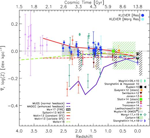
Compilation of metallicity gradients plotted as a function of redshift (or, equivalently, the age of the Universe). The blue points mark the results derived in this work, where we distinguish between resolved (blue circles) or marginally resolved (light blue circles) gradients. Additional measurements of metallicity gradients from previous works, derived with different techniques on both local and high-z galaxies, are included with different symbols/colours as explained in the legend. The metallicity gradients by Carton et al. (2018) are based on MUSE observations of 0.1 < z < 0.8 galaxies, for which we report the spread in their measurements both in redshift and ∇Z. The sample from Queyrel et al. (2012) reports SINFONI observations of z ∼ 1.2 galaxies from the MASSIV survey, while Stott et al. (2014) reports KMOS observations of z ∼ 0.8 galaxies from the HiZELS survey. For these works, we report the average and 1σ dispersion for their metallicity gradient measurements at the mean redshift of each sample. The grey shaded areas, instead, represent the spread in the metallicity gradients measured in the framework of the KMOS3D Survey within three different redshift intervals and presented by Wuyts et al. (2016). Jones et al. (2013) and Leethochawalit et al. (2016) report observations conducted with AO-assisted spectroscopy with OSIRIS at Keck on gravitationally lensed systems, while Jones et al. (2015a), Wang et al. (2017), and Wang et al. (2019) are based on HST-grism slitless spectroscopy of lensed galaxies behind the Frontier Fields clusters as part of the GLASS program (Treu et al. 2015). The metallicity gradients at z > 3 from Troncoso et al. (2014) are based on SINFONI observations in the framework of the AMAZE and LSD programs (Maiolino et al. 2008; Mannucci et al. 2009). For what concerns the metallicity gradients in the local Universe, we show the average of local gradients for isolated (filled square) and interacting (open square) systems from Rupke et al. (2010b). We also report the time evolution of metallicity gradients for the Milky Way, M33 and M81, as inferred from abundances computed for H ii regions (open half-circles) and planetary nebulae (PNe, filled half-circles, associated with older stellar population progenitors) and presented in Magrini et al. (2009, 2010), Stanghellini & Haywood (2010), Stanghellini et al. (2014), and Stanghellini & Haywood (2018). The predictions from MUGS and MaGICC cosmological simulations reported in Gibson et al. (2013a), which track the evolution of a typical disc galaxy implementing two different feedback modes, are shown with a dashed purple line for the enhanced feedback scenario and with a straight purple line for the normal feedback scenario, respectively. The black hatched regions cover instead the predictions of metallicity gradients at four different epochs (i.e. z = 0, 0.8, 1.5, and 2) from the FIRE simulations, as presented by Ma et al. (2017). The brown curve shows the predicted cosmic evolution of the metallicity gradient from the Spitoni, Matteucci & Marcon-Uchida (2013) modelling of M31, and in light green those from the chemical evolution models by Mollá et al. (2018). Finally, the predictions of chemical evolution models by Mott, Spitoni & Matteucci (2013) assuming constant (solid line) and variable (dot–dashed line) star formation efficiencies are plotted in red. Our results are consistent with little or no evolution of the metallicity gradients with redshift, in better agreement with predictions by simulations and models including strong feedback mechanisms and/or gas radial flows in place.
We can compare these results with the predictions from cosmological hydrodynamical simulations, which trace the gas-phase metallicity of disc galaxies from z ∼ 2 to the present day under different feedback modes in the framework of the MUGS (Stinson et al. 2010) and MaGICC (Gibson et al. 2013b) schemes. We show the evolutionary track for the simulated galaxy g15784 under both normal and enhanced feedback conditions. The ‘normal’ feedback scenario, in which 10–|$40 {{\ \rm per\ cent}}$| of the energy from each supernova is used to heat the surrounding ISM, predicts steeper metallicity gradients at earlier redshifts (i.e. |${\sim}-0.2 \, \text{dex kpc}^{-1}$|), which become flatter over cosmic time. The totality of our measurements and even the largest part of those reported in the literature are inconsistent with this scenario, with just a few examples of observed gradients that match its predictions at redshifts higher than 1.5 (Jones et al. 2013; Wang et al. 2017). The enhanced feedback scheme instead, where outflows redistribute energy and recycle ISM material over larger galactic scales, with preferential re-accretion into the outer regions (i.e. metal recycling), is characterized by a milder evolution with a progressive (minimal) flattening of the metallicity gradients with increasing redshift. Our results, together with the majority of previous indications from the literature, seem to point towards this latter regime, which suggests that, at high-z, stronger star formation feedback is in place, causing flatter gradients due to rapid and efficient recycling of enriched gas and redistribution of the ISM, which occurs on time-scales shorter than those related to star formation and metal enrichment. Within the context of the high-resolution FIRE simulations, Ma et al. (2017) presented gas-phase metallicity maps and measured radial gradients within 0.25–1 R902 for a sample of simulated galaxies up to z ∼ 2. They are capable of predicting a variety of metallicity distributions and gradients at each cosmic epoch (represented by the black hatched regions in Fig. 8), spanning from strongly negative ones in ordered discs to flatter gradients in more perturbed systems affected by mergers and significant gas flows, which mix the ISM on large galactic scales (≲10 kpc) on relatively short time-scales (∼10–50 Myr), nicely reproducing the scatter in the observational results.
In Fig. 8, we also show the prediction for the metallicity gradient of M31 at different redshifts according to the Spitoni et al. (2013) chemical evolution model (solid brown line), which assumes no gas threshold on star formation, an inside-out formation of the disc, constant star formation efficiency along the disc, and radial gas flows; this model is consistent with enhanced-feedback simulation schemes in prescribing a mild steepening of the gradient with time. Interestingly, no or little evolution in the predicted metallicity gradients can be achieved also by purely or semi-analytical chemical evolution models that do not include any prescription about feedback processes mixing up the gas. The models from Mollá & Díaz (2005) [then revisited by Mollá et al. (2017, 2018), green dashed line], for example, assuming an inside-out disc growth, an ISM structured as a multiphase mix of diffuse gas and cold clouds and prescribing star formation efficiencies, stellar yields, gas infall rates, and atomic-to-molecular hydrogen conversion factors, predict flat metallicity gradients at all redshifts within 2.5 effective radii in disc galaxies, with no assumption on radial gas mixing.
Among our galaxies, we report several examples of positive, ‘inverted’ metallicity gradients, despite only three determined with a >3σ significance (i.e. sp6, ph3912, and ph6532, with R2248_LRb_p3_M4_Q3_94__1 at 2.8σ). Previous claims of such gradients have been reported both at the same redshifts (Wuyts et al. 2016; Wang et al. 2019) and at earlier epochs (z >3), mostly in seeing-limited data of unlensed galaxies (Cresci et al. 2010; Troncoso et al. 2014); similarly to these findings, the central metal-poor regions in our galaxies are co-spatial with the regions of highest SFR density (and hence higher gas fractions). These observations have been interpreted as evidence of cold flows of pristine gas into the central regions of such galaxies, which both fuels new star formation episodes and dilutes the metallicity (Dekel et al. 2009; Cresci et al. 2010). An alternative explanation consists in considering these galaxies affected by strong feedback processes, in the form of outflows that rain material from the inner regions back down in the outskirts of the galaxy (the so-called ‘galactic fountain’ effect, Fraternali & Binney 2008; Werk et al. 2011). This process, whose primary effect results in an average flattening of the abundance gradients, can contribute in some cases to invert the gradient itself, as the highest mass-loss rate is observed in the central regions (Wang et al. 2019). However, the impact of these outflows does not seem to be powerful enough to represent the dominant contribution to such a flattening for the ensemble population, since the measured mass outflow rates are often too small (Cresci et al. 2010; Troncoso et al. 2014). In the framework of chemical evolution models, Mott et al. (2013) managed to reproduce inverted gradients at z > 1 assuming the inside-out formation of the disc, a threshold in the gas density for star formation, a variable star formation efficiency (SFE) along the disc, and the presence of radial flows with varying speed. In particular, they find the velocity pattern for radial gas flows to be a crucial parameter in shaping the chemical evolution of the disc, and that a constant star formation efficiency along the disc is needed to reproduce the observed inverse gradients (solid red line in Fig. 8).
Finally, it is worth noting here that the large majority of currently available results rely on a variety of different indicators for metallicity determination: many of them are derived only from nitrogen-based diagnostics ([N ii]/H |$\alpha$|, in particular, being one of the most easily accessible at high-z), some from purely oxygen-based ones. Moreover, besides the fact that the metallicity gradients shown in Fig. 8 are obtained with different diagnostics, the latter are sometimes even based on different calibration methods (e.g. Te versus photoionization modelling). This means not only that the absolute metallicity estimates could disagree between various methods, but also that the dynamic range of possible values spanned by the calibration itself could be different, which might translate in a change of the slope of the calibrated relation. In general, theoretical calibrations provide a wider range of possible metallicities with respect to Te-based methods, even when considering the same set of strong-line ratios, as they often provide higher normalizations in the high-metallicity regime. Therefore, the use of different diagnostics/calibrations could introduce systematics in the slope of the inferred gradients. However, given the generally small range of abundances spanned by individual regions across a galaxy (very strong gradients are rare), and considering that relative metallicity measurements are always much more robust than absolute ones, this effect is likely to be negligible in the majority of cases, making the comparison of samples derived with different techniques more fair.
4.4 Correlation with stellar mass and SFR
We discuss here whether the metallicity gradients correlate with global galaxy properties. As previously mentioned, the simulation of the inside-out growth of galaxies predicts initial steep negative gradients that flatten at later times, whereas observed positive or flat gradients are predicted by simulations and models as due to efficient re-accretion and gas mixing processes (e.g. Gibson et al. 2013b; Mott et al. 2013). In particular, the sSFR (sSFR = SFR/M⋆) is a measured quantity that holds information about galaxy star formation history: Galaxies exhibiting a high sSFR are experiencing a starbursting phase and might be in an early stage of their cosmic evolution, possibly fuelled by inflowing gas into their central regions and affected by strong feedback episodes. One can therefore expect that signatures of this process might also be observed in the metallicity gradients, in the sense that galaxies with higher sSFR exhibit on average flatter (or more positive) gradients than those characterized by a low sSFR.
In the upper panel of Fig. 9, we plot the metallicity gradients sample as a function of sSFR, along with gradients from previous works at z ≳ 0.8 (i.e. Queyrel et al. 2012; Swinbank et al. 2012; Jones et al. 2013; Stott et al. 2014; Troncoso et al. 2014; Jones et al. 2015a; Wuyts et al. 2016; Wang et al. 2017, 2019)). We exploited the sklearn python package to perform a robust linear regression and quantify the level of correlation: The result is shown with the black line in Fig. 9, with the shaded region indicating the r.m.s. of the fit. The slope of the relation is equal to 0.013 ± 0.004 (i.e. 3.2σ from being flat), with an r.m.s. of 0.05 dex, suggesting that a correlation between metallicity gradients and sSFR might be present in the sense of most active galaxies (i.e. higher sSFR) being characterized by flatter or positive gradients. This is consistent with the trend originally found by Stott et al. (2014) and the predictions of the FIRE simulations in Ma et al. (2017). Nevertheless, the level of correlation is very mild, as a Spearman test gives only ρ = 0.29 with a |$99.9{{\ \rm per\ cent}}$| level of confidence.

Metallicity gradients as a function of global sSFR (upper panel) and stellar mass (bottom panel). The sample includes both objects from KLEVER and additional gradients from previous works on z ≳ 0.8 sources; symbols and colours are the same as in Fig. 8. A robust linear regression fit to the data is shown in black in both the panels, with the RMS region marked in grey. A mild correlation is present between metallicity gradients and both quantities, in the sense of a positive trend with increasing sSFR and a negative trend with increasing M⋆, significant at 3.2σ and 2.7σ and with a Spearman correlation coefficient ρ = 0.29 and −0.25, respectively. In the bottom panel, the trend between gradients and stellar mass in the local Universe (inferred from a sample of galaxies in MANGA, Belfiore et al. 2017) is traced by the black line.
We also investigate whether our metallicity gradients correlate with total stellar mass in the bottom panel of Fig. 9. We perform the same linear regression and find a slightly negative slope (−0.013 ± 0.005), significant at the 2.6σ level. A Spearman correlation test gives ρ = −0.25 with the |$99.9{{\ \rm per\ cent}}$| of confidence. Again, this is consistent with previous observational assessments (Stott et al. 2014; Wuyts et al. 2016) and simulations (Ma et al. 2017). In the local Universe, a clear trend of metallicity gradients with stellar mass is observed, as recently shown, for example, by Belfiore et al. (2017) for a large sample of galaxies within the MANGA survey: Less massive systems are characterized by flatter metallicity gradients, steepening (i.e. becoming negative) with increasing stellar mass up to 1010.5 M⊙, before flattening again at higher masses (especially in their central regions). In the framework of the classical inside-out growth scenario, and assuming a radially decreasing star formation efficiency, feedback and/or gas recycling mechanisms are required to reproduce the observed flattening of the gradients at low masses (see also Belfiore et al. 2019).
As also seen in Section 3.3, the sample analysed in this paper is distributed across a wide region of the M⋆–SFR plane, although being preferentially constituted by higher sSFR galaxies than representative samples at the corresponding redshifts, especially at z > 2. Fig. 10 shows how the metallicity gradient sample analysed in this paper and the compiled sample from the literature are distributed as a function of |$\rm \Delta$|SFMS, defined as the distance from the SFMS computed at each source redshift, adopting the redshift-dependent parametrization of Speagle et al. (2014). In the bottom panel of Fig. 10, we investigate the correlation between metallicity gradients and |$\rm \Delta$|SFMS. When normalized to the main sequence at each redshift, the correlation is found to be weaker compared to the trends previously discussed, with ρ = 0.20 and a slope significantly different from being flat only at the 2σ level.

Upper panels: Stacked histograms of the distribution in |$\rm \Delta$|SFMS, defined as the distance from the SFMS of Speagle et al. (2014) at the mean redshift of each reference sample, for the KLEVER galaxies hereby analysed (left-hand panel) and the compiled sample from the literature at z ≳ 0.8 (right-hand panel). Bottom panel: Metallicity gradients as a function of |$\rm \Delta$|SFMS. Compared to the trends shown in Fig. 9, the significance is reduced to ∼2σ, with a Spearman coefficient ρ = 0.20.
In light of the trends shown and discussed above, we note that it might be therefore more likely for KLEVER galaxies to show flatter gradients compared to the rest of the complied sample, although flat gradients are found at all M⋆ and SFR within our sample. None the less, the full high-z sample shown in Fig. 8 is almost uniformly distributed in |$\rm \Delta$|SFMS, hence the overall bias introduced in the interpretation of the cosmic evolution of the gradients is supposed to be minimal. The only exception is the sample of z > 3 galaxies from Troncoso et al. (2014), which appears to be constituted by galaxies lying systematically above the SFMS at that redshift. Therefore, it is possible that the incidence of inverted gradients in the population, as inferred from that particular sample, is overestimated, modulo the uncertainties associated with the parametrization of the SFMS at high redshifts, which should always be taken into account when performing this type of analysis.
Interestingly, Wang et al. (2017) report a few examples of steep, negative gradients (<−0.1 dex kpc−1) at low masses (i.e. M⋆ < 109M⊙) from their HST-grism spectroscopic survey of lensed galaxies, which deviate both from the average trend followed by the rest of the high-z sample and from the picture outlined in the local Universe. According to the authors, they could be interpreted as systems with a rapid and highly centrally concentrated star formation history and limited feedback mechanisms and are, to date, the only reported systems that fit the ‘purely inside-out growth’ scenario of mass assembly. However, a larger number of robust measurements of metallicity gradients in low-mass galaxies are required in order to carefully estimate the occurrence rate of such systems and whether they might represent a different galaxy population. In this sense, the full KLEVER sample will strongly contribute to increase the statistics in the low-mass regime.
4.5 Are radial gradients always meaningful?
A first look at the derived metallicity gradients reveals how the vast majority of the sample is characterized by radial gradients consistent with being flat within their uncertainties. However, we note that some of the metallicity maps are characterized by the presence of non-axisymmetric patterns, revealing a more complex distribution in the level of chemical enrichment. This means that a formally flat radial metallicity gradient may be either the consequence, on one hand, of a fairly homogeneous metallicity map, resulting from the mixing of the ISM on large scales or from a flat, extended star formation profile, while on the other hand can hide the presence of non-radial variations (even on ∼ kpc scales) that are washed out (producing a flat gradient) when azimuthally averaged. On average, the maximum metallicity variation between different regions in most of our galaxies is around ∼0.1–0.2 dex; however, when these regions are not symmetrically distributed around the galaxy centre, they might be hidden by the azimuthal averages and the resulting gradient would be artificially flatter. Interestingly, some of those galaxies showing irregularities in their emission-line maps and/or velocity fields present clear signatures of disturbed morphology in the HST images, which could reveal ongoing interactions or suggest clumpy structures in their discs. A few examples are discussed in the following and shown in Fig. 11, where both image-plane and source-plane HST images, velocity fields, and metallicity maps are reported for four different systems.

Examples of systems showing disturbed morphologies, kinematics, and metallicity maps. From left to right: HST F160W image, HST F814W image, reconstructed HST F814W source-plane image, H α velocity field, and metallicity map are shown for four galaxies analysed in this work. These galaxies present extended H α emission or secondary peaks misaligned from the bulk of the underlying H-band continuum. These regions of intense off-nuclear H α emission may be either associated with episodes of recent star formation occurring in compact clumps that form in the turbulent gas-rich disc or the results of merger events that, however, cannot always be obviously confirmed from the velocity fields. These regions are often characterized by a different level of chemical enrichment compared to the bulk of the system. In each panel, the overlaid contours encompass the |$50{},68{}, 85{}$|, and |$97{{\ \rm per\ cent}}$| of the H α emission, while the black crosses mark the position of the peak of the underlying HST continuum image.
The complex kinematics seen in the velocity fields of sp15 suggests a primary galaxy (associated with the H |$\alpha$| peak and with a clear velocity gradient) interacting with a fainter companion responsible for the redshifted H |$\alpha$| emission towards the bottom right part of the image. The H |$\alpha$| emission is elongated towards the north-east, co-spatial with the ‘tail’ visible in the HST images. The metallicity map is strongly irregular, with an apparent spatial anticorrelation between the intensity of the H |$\alpha$| and the metallicity. However, the azimuthal asymmetry is partially washed out when averaging, with the final gradient equal to −0.005 ± 0.010. A similar behaviour can be seen for the galaxy sp1, which shows the presence of multiple components, clearly visible in the F814W image, with the centroid of the extended H |$\alpha$| emission misaligned from the peak of the F160W continuum, more representative of the stellar mass density distribution. The velocity map is nevertheless quite regular and does not show any clear deviation from an ordered disc-like rotation pattern (making its interpretation often non-trivial in seeing-limited data; see e.g. Simons et al. 2019). A clear linear gradient in the metallicity map can be seen from the most active, metal-poor region in the south-east area to the more metal-rich region towards the north-west direction, which is associated with the main disc component (as marked by the peak of H-band continuum image); however, the gradient is lost if radially averaging around the centroid of the emission in the system. MUSE_SW_461-99-99 is characterized by the presence of a distinct H |$\alpha$| blob in the north-west region of the image-plane map (south-west in the source plane), which is not detected in the KMOS H-band continuum map nor can be clearly associated with any visible structure in the broad-band HST-F160w image (nor in the de-lensed velocity field). However, the HST-F814w image reveals a more complex morphology, with an offset component (likely a companion galaxy) aligned with the secondary H |$\alpha$| peak. It is worth noting how in this case the metallicity of the region co-spatial with the secondary H |$\alpha$| blob is significantly lower than that of the central galaxy. Finally, R2248_LRb_p1_M3_Q4_58__2 presents a bright, elongated knot westward (∼1.5 kpc far) of the centre in the F814W image, which is not detected in H-band continuum. However, the centroid of the H |$\alpha$| emission is shifted in the same direction, and the region is characterized by a slightly enhanced level of enrichment.
As we have seen, these configurations may be either related to the presence of close interacting companions or even suggest that different processes, occurring on shorter time-scales than secular processes and mainly associated with gas flows, could contribute to the complexity seen in some of the 2D metallicity maps. High-resolution simulations of disc galaxies (Milky Way-like at redshift zero) have shown in fact that strong fluctuations in their star formation history and gas outflow rate occurring on relatively short time-scales (i.e. ≲1 Gyr) can induce significant fluctuations in the gas-phase metallicity maps and hence in the derived radial gradients (Ma et al. 2017). In general, at the peak of the cosmic star formation history (z ∼ 1.5–2.5, the epoch probed by KLEVER), galaxies are often characterized by irregular morphologies and their emission-line luminosity might be dominated by the presence of young, massive star-forming clumps (Elmegreen 2009; Förster Schreiber et al. 2011; Genzel et al. 2011). Recent cosmological simulations by Ceverino et al. (2016) also show that in |$50 {{\ \rm per\ cent}}$| of cases at redshifts lower than 4, pristine gas accretion from the cosmic web can give rise to the formation of local star-forming clumps and subsequent drop in metallicity (|${\sim}0.3 \rm ~dex$|) compared to the surrounding ISM. They further assert that the accretion should be rapid enough to sustain such a metallicity drop, as the turbulence mixing would dissolve these features within a few disc dynamical time-scales. Another possibility is that these clumps may form within their gas-rich discs due to gravitational instabilities (Bournaud, Elmegreen & Elmegreen 2007; Elmegreen, Bournaud & Elmegreen 2008; Genzel et al. 2008); in this case, they might leave a different imprint on the metallicity maps, showing similar level of chemical enrichment to those of the material from which they have formed. The presence of such regions of different star formation and chemical enrichment histories within the same galaxy may reflect itself in the azimuthal asymmetries seen in some of the metallicity maps, despite the impossibility to resolve them spatially given the intrinsic limitations of seeing-limited observations in reaching the required resolution (∼100 pc, Tamburello et al. 2017). Nonetheless, recent observations conducted with SINFONI AO-assisted spectroscopy have also reported similar asymmetries in the distribution of the [N ii]/Hα line ratio in z∼ 2 galaxies (Förster Schreiber et al. 2018). Therefore, although azimuthally averaged gradients are still useful and commonly adopted as a benchmark for theoretical predictions, this suggests that only the full characterization of the spatial distribution of the heavy elements within a galaxy (i.e. the 2D metallicity maps) can ultimately provide the key to resolve the interplay between physical processes occurring on local scales (gas accretion, gas flows, turbulent mixing, etc.) and global, secular processes, constraining their role in shaping the formation of galactic discs at these epochs.
5 SUMMARY AND CONCLUSIONS
We have analysed a sample of gravitationally lensed galaxies between redshifts 1.2 < z < 2.5, observed with KMOS and SINFONI as a first part of the KLEVER Large Programme. The observations conducted in the YJ, H, and K bands provided spatially resolved mapping of many rest-frame optical nebular emission lines, allowing us to assess different ISM properties in these objects on both global and local scales. In particular, in this work, we have constrained gas-phase metallicities by simultaneously adopting different strong-line diagnostics and calibrations tied to the Te abundance scale. The sample covers a range of 108.5–1010.5 M⊙ in stellar mass and ∼1–200 M⊙ yr−1 in SFR, sampling galaxies on above and below the SFMS at these redshifts, with a slight bias towards high sSFRs especially at z > 2. On global scales (i.e. from the analysis of their integrated spectra), the galaxies analysed are consistent with the observed evolution in the BPT diagrams and in the mass–metallicity relation reported in previous studies (Figs 5 and 6).
In this paper, we mainly focused on the analysis of metallicity gradients. We have exploited robust lens modelling of foreground sources (mainly galaxy clusters) to obtain source-plane emission-line maps with a typical resolution of |${\sim}3\ \, \text{kpc}$|, from which we have derived metallicity maps and extracted radial metallicity gradients by means of azimuthal averages within elliptical apertures defined according to the shape of the source-plane PSF (e.g. Fig. 7). The main conclusions drawn in this paper are summarized as follows:
The |$86{{\ \rm per\ cent}}$| of our galaxy sample presents radial metallicity gradients shallower than |$0.05\ \rm dex\, kpc^{-1}$| (|$72{{\ \rm per\ cent}}$| within |$0.025\ \rm dex\, kpc^{-1}$|), with |$89{{\ \rm per\ cent}}$| of the gradients consistent with being flat within a 3σ uncertainty (|$67{{\ \rm per\ cent}}$| within 1σ). This is in agreement with the majority of previous results reported in the literature that investigated metallicity gradients at z ∼1–2.5, despite the diversity of observational techniques and diagnostics adopted (Fig. 8). A comparison with cosmological simulations that explore the effect of different feedback modes suggests a scenario where efficient mixing processes, which redistribute a significant amount of gas over large scales, are in place at these epochs (Gibson et al. 2013b). However, predictions from analytical models, which assume fairly constant star formation profiles and no prescriptions about radial gas mixing, are also broadly consistent with the observed distribution of metallicity gradients observed in the galaxy population at z ∼1–2.5 (Mollá et al. 2019). Galaxies showing a relatively homogeneous metal distribution across large spatial scales might also be consistent with a scenario of uniform disc mass assembly.
Three sources in the sample are characterized by significantly (i.e. above 3σ) positive (‘inverted’) metallicity gradients. Similarly with previous findings in the literature (Cresci et al. 2010; Troncoso et al. 2014) , in these galaxies the central metal-poor regions are associated with the highest level of H |$\alpha$| emission, hence with the highest SFR surface density, suggesting recent accretion of pristine gas. Alternatively, chemical evolution models assuming a constant SFE along the disc and allowing for large variations in the velocity of radial gas flows have also shown to be able to predict an ‘inversion’ of the metallicity gradients (Mott et al. 2013).
We explored the correlation between the sSFR and metallicity gradients at z > 0.8, extending the relation towards the highest sSFRs probed by our sample (Fig. 9, upper panel). We find a mild trend in which galaxies with a higher sSFR exhibit flatter or ‘more positive’ gradients, with a significance of 3.2σ, in agreement with previous findings (Stott et al. 2014; Wuyts et al. 2016). When normalizing the SFR to that expected from the SFMS at each redshift, the significance of the trend reduces to 2σ (Fig. 10). We have found a milder, negative correlation between metallicity gradients and stellar mass (significant at the 2.7σ level, lower panel of Fig. 9), consistent though with the trend followed in the local Universe (i.e. gradients steepening with increasing stellar mass, Belfiore et al. 2017).
Despite the apparent radial invariance, some of our galaxies exhibit complex patterns in the metallicity maps, with variations in log(O/H) of the order of 0.1–0.2 dex on kpc scales, which are, however, not symmetrically distributed around the galaxy centre (Fig. 11). In these cases, flat gradients might artificially arise from azimuthal averages, washing out and therefore hiding the presence of regions with different levels of chemical enrichment. Strong fluctuations in the star formation history and outflow rates or local episodes of gas accretion occurring on short time-scales could explain the observed irregular morphologies. This warns against using radial gradients as the only constraints for galaxy evolution models. Extracting more information from the full 2D metallicity maps is key to discriminate between the contribution that different local processes (like gas recycling via stellar feedback, pristine gas accretion, turbulent mixing, and merger events) have in shaping the observed morphologies.
In conclusion, mutual interactions between star formation and different processes involving efficient radial mixing driven by intense galactic feedback or merger events could strongly affect the complex morphology of the maps and the average radial flattening of the gradients that we see at these epochs. A more comprehensive and self-consistent view of spatially resolved metallicity properties in high-z galaxies will be possible as soon as the KLEVER Programme is completed, comprising a larger sample spanning a wider range in stellar masses and SFRs. The complexity revealed by current-generation IFU instruments is also paving the way for observations with next-generation facilities like NIRSPEC on JWST and ERIS (the AO-assisted Enhanced Resolution Imager and Spectrograph, aimed at substituting SINFONI on the VLT from 2020, Davies et al. 2018), which will offer in the near future the opportunity to probe the metal distribution in high-redshift galaxies with unprecedented detail, helping to discriminate between different theoretical predictions and setting new and powerful constraints for cosmological simulations and chemical evolution models.
SUPPORTING INFORMATION
In particular, in Appendix A, we address the potential systematics associated with the choice of the radial binning scheme adopted in the source plane to derive the metallicity gradients. In Appendix B, instead, we present the emission-line maps, metallicity maps, and metallicity gradients for the full metallicity gradients sample. Finally, in Appendix C, we report the full version of Tables 2–4 presented throughout the paper.
Please note: Oxford University Press is not responsible for the content or functionality of any supporting materials supplied by the authors. Any queries (other than missing material) should be directed to the corresponding author for the article.
ACKNOWLEDGEMENTS
Based on observations made with ESO Telescopes at the La Silla Paranal Observatory under programme IDs 083.A-0918(A), 083.B-0108(A), 090.B-0313(A), 092.A-0426(A), 092.B-0677(A), 094.A-0279(A), 095.B-0480(A), and 197.A-0717(A). The mass models for the lensed galaxies in galaxy clusters were developed by Zitrin et al. (2009, 2013), and obtained through the Hubble Space Telescope Archive, as a high-end science product of the CLASH (Postman et al. 2012) and Frontier Fields (Lotz et al. 2017) programs.
MC and RM acknowledge support by the Science and Technology Facilities Council (STFC) and from ERC Advanced Grant 695671 ‘QUENCH’. GC acknowledges the support by INAF/Frontiera through the ‘Progetti Premiali’ funding scheme of the Italian Ministry of Education, University, and Research; GC has been also supported by the INAF PRIN-SKA 2017 program 1.05.01.88.04. MC acknowledges support from a Royal Society University Research Fellowship. CC acknowledges funding from the European Union’s Horizon 2020 research and innovation programme under the Marie Sklodowska-Curie grant agreement no. 664931. YP acknowledges support from the National Key Program for Science and Technology Research and Development under grant number 2016YFA0400702, and the NSFC grant nos. 11773001 and 11721303.
This work utilizes gravitational lensing models produced by PIs Bradac, Natarajan and Kneib (CATS), Merten and Zitrin, Sharon, Williams, Keeton, Bernstein and Diego, and the GLAFIC group. This lens modelling was partially funded by the HST Frontier Fields program conducted by STScI. STScI is operated by the Association of Universities for Research in Astronomy, Inc. under NASA contract NAS 5-26555. The lens models were obtained from the Mikulski Archive for Space Telescopes (MAST).
Footnotes
Downloadable from the Frontier Fields and CLASH models repository.
The radius enclosing |$90{{\ \rm per\ cent}}$| of the star formation within 10 kpc.
