


ABSTRACT
We present spatially resolved Echelle spectroscopy of an intervening Mg ii–Fe ii–Mg i absorption-line system detected at zabs = 0.73379 towards the giant gravitational arc PSZ1 G311.65–18.48. The absorbing gas is associated with an inclined disc-like star-forming galaxy, whose major axis is aligned with the two arc-segments reported here. We probe in absorption the galaxy’s extended disc continuously, at ≈3 kpc sampling, from its inner region out to 15× the optical radius. We detect strong (|$W_0^{2796}\gt 0.3$|Å) coherent absorption along 13 independent positions at impact parameters D = 0–29 kpc on one side of the galaxy, and no absorption at D = 28–57 kpc on the opposite side (all de-lensed distances at zabs). We show that (1) the gas distribution is anisotropic; (2) |$W_0^{2796}$|, |$W_0^{2600}$|, |$W_0^{2852}$|, and the ratio |$W_0^{2600}\!/W_0^{2796}$|, all anticorrelate with D; (3) the |$W_0^{2796}$|–D relation is not cuspy and exhibits significantly less scatter than the quasar-absorber statistics; (4) the absorbing gas is co-rotating with the galaxy out to D ≲ 20 kpc, resembling a ‘flat’ rotation curve, but at D ≳ 20 kpc velocities decline below the expectations from a 3D disc-model extrapolated from the nebular [O ii] emission. These signatures constitute unambiguous evidence for rotating extra-planar diffuse gas, possibly also undergoing enriched accretion at its edge. Arguably, we are witnessing some of the long-sought processes of the baryon cycle in a single distant galaxy expected to be representative of such phenomena.
1 INTRODUCTION
Models and simulations that describe the various components and scales of the baryon cycle around galaxies remain to be tested observationally. Such a task poses a serious challenge, though, as most of the ‘action’ occurs in the diffuse circumgalactic medium (CGM), i.e. at several optical radii from the host galaxy scales (e.g. Tumlinson, Peeples & Werk 2017). Traditionally, observations of the CGM at 10–100 kpc scales have been based on the absorption it imprints on background sources, primarily quasars (e.g. Nielsen et al. 2013a; Chen 2017; Prochaska et al. 2017; Tumlinson et al. 2017, and references therein) but also galaxies (Steidel et al. 2010; Diamond-Stanic et al. 2016; Rubin et al. 2018b), including the absorbing galaxy itself (Martin 2005; Kornei et al. 2012; Martin et al. 2012). Such techniques have yielded a plethora of observational constraints and evidence for a connection between a galaxy’s properties and its CGM.
Galaxies studied through these methods, nevertheless, are probed by single pencil beams; therefore, to draw any conclusions that involve the spatial dependence of an observable requires averaging absorber properties (Chen et al. 2010; Nielsen, Churchill & Kacprzak 2013b) or stacking spectra of the background sources (Steidel et al. 2010; Bordoloi et al. 2011; Rubin et al. 2018a,c). A complementary workaround is to use multiple sightlines through individual galaxies. Depending on the scales, the background sources can be binary or chance quasar groups (Martin et al. 2010; Bowen et al. 2016) or else lensed quasars (Smette et al. 1992; Lopez et al. 1999, 2005, 2007; Rauch et al. 2001; Ellison et al. 2004; Chen et al. 2014; Zahedy et al. 2016). Despite the paucity of the latter, lensed sources are able to resolve the CGM of intervening galaxies on kpc scales, albeit at a sparse sampling. More recently, Lopez et al. (2018) have shown that the spatial sampling can be greatly enhanced by using giant gravitational arcs. Comparatively, these giant arcs are very extended (e.g. Sharon et al. 2019) and thus can probe the gaseous halo of individual galaxies on scales of 1–100 kpc at a continuous sampling, nicely matching typical CGM scales. Such an experimental setup therefore removes potential biases introduced by averaging a variety of absorbing galaxies.
Following on our first tomographic study of the cool CGM around a star-forming group of galaxies at z ≈ 1 (Lopez et al. 2018, hereafter ‘Paper I’), we here present spatially resolved spectroscopy of a second giant gravitational arc. We pool together Echelle and integral-field (IFU) spectroscopy of the brightest known gravitational arc to date, found around the cluster PSZ1 G311.65–18.48 (a.k.a. the ‘Sunburst Arc’; Dahle et al. 2016; Rivera-Thorsen et al. 2017, 2019; Chisholm et al. 2019). We apply our technique to study the spatial extent and kinematics of an intervening Mg ii–Fe ii–Mg i absorption-line system at z = 0.73379. Due to a serendipitous arc/absorber geometrical projection on the sky, we are able to spatially resolve the system all along the major axis of a host galaxy that may be exemplary of the absorber population at these intermediate redshifts.
The paper is structured as follows. In Section 2, we present the observations and describe the different data sets. In Section 3, we describe the reconstructed absorber plane and assess the meaning of the absorption signal. In Section 4, we present the emission properties of the identified absorbing galaxy. In Section 5, we provide the main analysis and results on the line strength and kinematics of the absorbing gas. We discuss our results in Section 6 and present our summary and conclusions in Section 7. Details on data reduction and models are provided in the Appendix. Throughout the paper, we use a ΛCDM cosmology with the following cosmological parameters: H0 = 70 km s−1 Mpc−1, Ωm = 0.3, and ΩΛ = 0.7.
2 OBSERVATIONS AND DATA REDUCTION
2.1 Experimental setup
PSZ1 G311.65–18.48 extends over ≈60 arcsec on the sky (Fig. 1) and results from the lensing of a z = 2.369 star-forming galaxy by a cluster at z = 0.443 (Dahle et al. 2016). According to archival VLT/MUSE data, an intervening Mg ii absorption-line system at z = 0.73379 appears in the spectra of one of northernmost segments of the arc. The same data reveal nebular [O ii] emission at the same redshift from a nearby galaxy, which we consider to be the absorbing galaxy (hereafter referred to as ‘G1’). To thoroughly study this system, in this paper we exploit three independent data sets: (1) medium-resolution IFU data obtained with VLT/MUSE, which we use to constrain the emission-line properties of G1; (2) Hubble Space Telescope (HST) imaging, which we largely use to (a) build the lens model needed to reconstruct the absorber plane and (b) constrain the overall properties of G1 based on its continuum emission; and (3) medium-resolution Echelle spectra obtained with Magellan/MagE, which we use to constrain the absorption-line properties of the gas.
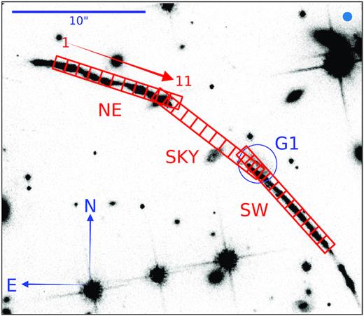
HST/ACS F814W-band image of the northern arc segments around PSZ1 G311.65–18.48. The three MagE slits (‘NE’, ‘SKY’, and ‘SW’) are indicated in red, along with our definition of ‘pseudo-spaxels’, and their numbering (for clarity only shown for the NE slit; see Section 2.4). The slit widths are of 1 arcsec, and their lengths are of 10 arcsec; we have divided each of them into 11 pseudo-spaxels of 1.0 arcsec × 0.9 arcsec each. The position of the absorbing galaxy (G1) is encircled in blue. The ground-based observations were performed under a seeing of 0.7 arcsec (represented by the beam-size symbol in the top-right corner).
2.2 VLT/MUSE
We retrieved MUSE observations of PSZ1 G311.65–18.48 from the ESO archive (ESO program 297.A-5012(A); PI Aghanim). The field comprising the arc segments shown in Fig. 1 was observed in wide-field mode for a total of 2966 s on the night of 2016 May 13 under good seeing conditions (0.7 arcsec). We reduced the raw data using the MUSE pipeline v1.6.4 available in esoreflex. The sky subtraction was improved using the Zurich Atmospheric Purge (zap v1.0) algorithm. We applied a small offset to the HST and MUSE fields to take them to a common astrometric system using as a reference a single star near G1. The spectra cover the wavelength range |$4\, 750$|–|$9\, 300$| Å at a resolving power |$R\approx 2\, 100$|. The exposure time resulted in an S/N that is adequate to constrain the emission-line properties of G1, but not enough for the absorption-line analysis, given the MUSE spectral resolution.
2.3 HST/ACS
HST observations of PSZ1 G311.65–18.48 were conducted on 2018 February 21 to 22, and 2018 September 2 using the F814W filter of ACS (GO15101; PI Dahle) and the F160W filter of the IR channel of WFC3 (GO15337; PI Bayliss), respectively. F814W observations consist of eight dithered exposures acquired over two orbits, totalling 5280 s. F160W observations were conducted in one orbit, using three dithered pointings totalling 1359 s.
These data were reduced using the drizzlepac software package.1 Images were drizzled to a 0.03 arcsec pixel−1 grid using the routine astrodrizzle with a ‘drop size’ (final_pixfrac) of 0.8 using a Gaussian kernel. Where necessary, images were aligned using the routine tweakreg, before ultimately being drizzled on to a common reference grid with north up.
2.4 Magellan/MagE
Spectroscopically, Magellan/MagE greatly outperforms MUSE in terms of blue coverage and resolving power; hence, these observations are central to the present study. Here, we provide a concise description of the observations (see Table 1 for a summary). More details on the observations and data reduction are presented in Appendix A.
Summary of Magellan/MagE observations.
| Slit | PA | Exposure time | Airmass | Seeing | Blind offsets | |
|---|---|---|---|---|---|---|
| (deg) | Individual (s) | Total (h) | (arcsec) | ( arcsec) | ||
| (1) | (2) | (3) | (4) | (5) | (6) | (7) |
| SW | 42.0 | 2700 + 3600 + 4500 | 3.0 | 1.6–1.7 | 0.6–0.7 | 4.19(E), 10.22(S) |
| SKY | 52.3 | 4200 | 1.2 | 1.7 | 0.7–0.9 | 9.64(E), 5.39(S) |
| NE | 72.0 | 3600 + 3600 | 2.0 | 1.5–1.6 | 0.6-0.7 | 16.51(E), 1.47(S) |
Note. (1) Slit name (see Fig. 1); (2) position angle of slit; (3) individual exposure times; (4) total exposure times; (5) airmass of the observations; (6) typical seeing FWHM of the observations; (7) acquisition blind offsets to the East (E) and South (S) from reference star at celestial coordinate (J2000) RA = 15h50m00s and Dec. = −78°10m57s.
We observed the two northernmost segments in PSZ1 G311.65–18.48 during dark-time on the first half-nights of 2017 July 20 and 21 (program CN2017B-57, PI Tejos). The weather conditions varied but the seeing was good (0.6−0.7 arcsec) and steady.
With the idea of mimicking integral-field observations, we placed three 1 arcsec × 10 arcsec slits (referred to as ‘NE’, ‘SKY’, and ‘SW’) along the two arc segments (see Fig. 1) using blind offsets. The ‘SKY’ slit was placed in a way that the northernmost/southernmost extreme of the slit has light contribution from the north-east/south-west arc segments, respectively, while the inner part is dominated by the actual background sky signal. Thus, the ‘SKY’ slit provides not only a reference sky spectrum for the ‘NE’ and ‘SW’ slits (both completely covered by the extended emission of the arc at seeing 0.7 arcsec; see Fig. 2), but it also provides independent arc signal at the closest impact parameters to G1 in each arc segment.

Zoom-in into the SW segment showing a MUSE image centred at the continuum around Mg ii absorption at ∼4848 Å. The MagE ‘SW’ and ‘SKY’ slits with their corresponding pseudo-spaxels (Section 2.4) are shown in red. The blue circle indicates the seeing FWHM. The green contours indicate a flux level of 5σ above the sky level. Since the observing conditions during the MUSE and the MagE observations were quite similar (e.g. dark nights, seeing ≈0.7 arcsec), such contours show that SW pseudo-spaxels #2 to #11 and SKY pseudo-spaxels #10 to #11 were fully illuminated by the source, while SW #1 was only partially illuminated by the source. Using the same method, all NE pseudo-spaxels appear to be illuminated by the source (not shown here).
The data were reduced using a custom pipeline (see details in Section A2). The spectra cover the wavelength range |$3\, 300$|–|$9\, 250$| Å at a resolving power |$R=4\, 500$|. For each slit, 11 calibrated spectra were generated using a 3 pixel spatial binning, corresponding to 0.9 arcsec on the sky (see Fig. 3). Such binning oversamples the seeing, making the spectra spatially independent. These spectra define 11 ‘pseudo-spaxels’ in each slit. The spectra were recorded into three data-cubes of a rectangular shape of 1 × 11 ‘spaxels’ of 1.0 arcsec × 0.9 arcsec each. Throughout the paper, we use the convention that the northernmost spaxel in a given slit is its ‘position 1’ (e.g. SW #1) and position numbers increase towards the South in consecutive order (see Figs 1 to 3).

Raw MagE 2D spectra obtained through the SW (upper panel) and NE (bottom panel) slits. Each exposure is |$3\, 600$| s long. Wavelength increases to the right and each spectral pixel corresponds to ≈22 km s−1. Both spectra are centred at λ ≈ 4850 Å, the expected position of Mg ii λλ2796, 2803 at z = 0.73379 (indicated by the arrows in the upper panel). Mg ii absorption is clearly seen all along the SW slit, but not in the NE slit. Moreover, the velocity shift and kinematical complexity of the Mg ii absorption seems to be a function of the spatial position with respect to G1, which is located around SW position # 2 (see also Fig. 5). The grid tracing the Echelle orders corresponds to the 11 spatial positions (pseudo-spaxels) described in the text, with numbers (indicated on the right margin) increasing from North to South. Each position is 0.9 arcsec along the slit, and the slit width used was 1.0 arcsec. A sky line at 4861.32 Å blocks partially the 2803 Å transition, unfortunately, but it otherwise aids the eye to follow the spatial direction on the CCD.
3 LENS MODEL AND ABSORBER-PLANE GEOMETRY
In this section, we describe the lens model used to reconstruct the absorber plane and to properly define impact parameters.
3.1 Lens model
The lens model is computed using the public software lenstool (Jullo et al. 2007). Our model includes cluster-scale, group-scale, and galaxy-scale haloes. The positions, ellipticities, and position angles of galaxy-scale haloes are fixed to the observed properties of the cluster-member galaxies, which are selected from a colour–magnitude diagram using the red sequence technique (Gladders & Yee 2000). The other parameters are determined through scaling relations, with the exception of the brightest cluster galaxy that is not assumed to follow the same scaling. Some parameters of galaxies that are near lensed sources are left free to increase the model flexibility. The parameters of the cluster- and group-scale haloes are set as free parameters. The model used in this work solves for six distinct haloes, and overall uses 100 haloes.
We constrain the lens model with positions and spectroscopic redshifts of multiple images of lensed background sources, selected from our HST imaging and lensing analysis in this field will be presented in Sharon et al. (in preparation).
The arc segments are highly magnified and appear at regions close to the critical curves, where the lensing uncertainties are significant. However, for the redshift of G1 this region is far enough from the strong lensing regime, so that the lensing potential and its derivatives are smooth (as can be seen in Fig. 4) and the uncertainties are reduced.

Magnification map at z = 0.73379 (displayed in the image plane). The contours correspond to the HST F814W image. We caution that this figure does not show the magnification of the giant arc itself, which is at a different source redshift.
3.2 Absorber-plane geometry
Fig. 5 shows a zoom-in region of the field around G1 in the image plane (top panel) and in the reconstructed absorber plane at z = 0.73379 (bottom panel). For clarity, only the SW spaxels are shown. In the absorber plane, each spaxel is ≈3 × 6 kpc2 in size.
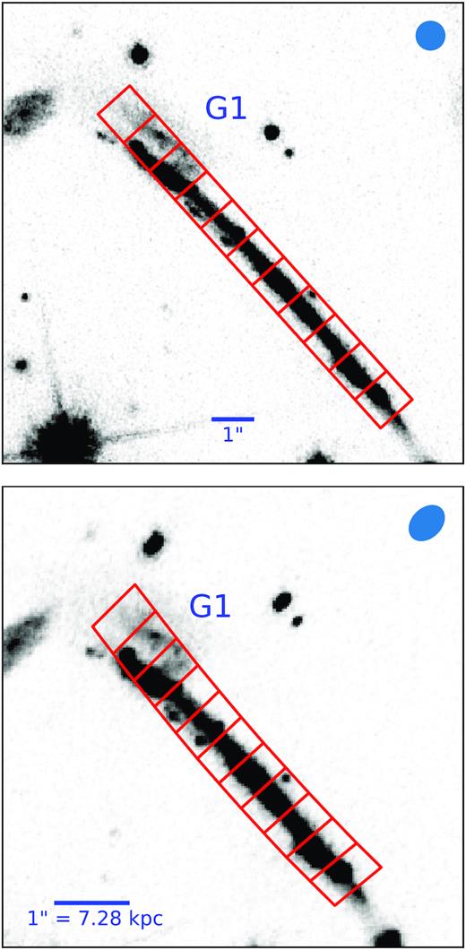
SW slit in the image plane (top) and in the reconstructed absorber plane (bottom). The ground-based observations were taken with a seeing of 0.7 arcsec (indicated by the beam size symbol in the top right of each panel); the background image is that of HST F814W-band image that highlights the location and morphology of G1 on both panels. In the absorber plane both the F814W image and the slit have been de-lensed to z = 0.73379 (see Section 3; including the shape of the PSF, which is used in Section 4.3 to run the galaxy emission model). In this plane, the separation between contiguous MagE spaxels is, on average, 3.2 kpc.
Impact parameters, D, are defined as the projected distance between the centre of a spaxel and the centre of G1. Impact parameters in arcseconds are defined in the reconstructed image. They are then converted to physical distances by using the cosmological scale at z = 0.73379 (1 arcsec = 7.28 kpc). For the sake of clarity, we arbitrarily assign negative or positive values depending on whether the spaxel is to the north-east or to the south-west of G1’s minor axis, respectively. Due to the particular alignment of galaxy and arc segments, the conversion between impact parameters in the image and in the reconstructed planes is almost linear (Fig. 6).
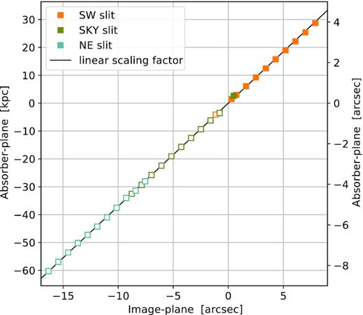
Impact parameters to G1, probed by the MagE spaxels in the image plane (horizontal scale) and in the absorber plane (vertical scales). Positions to the north-east of the G1 semiminor axis are assigned arbitrarily with negative values and are shown with open symbols. Note that the transformation from the image to the absorber plane is well approximated by a constant scale factor (the straight line in the figure). To convert angular distances into physical distances in the absorber plane a scale of 7.28 kpc arcsec−1 was used.
Our definition of impact parameter carries three sources of uncertainty. The first one comes from the lens model systematics and cosmology; we estimate this error to be ≈5 per cent, and therefore to dominate at large impact parameters. A second source of error comes from the astrometry, which introduces an error that dominates at low impact parameters. For instance, spaxel SW #1 in Fig. 5 does not apparently match any arc signal in the HST image. However, we do measure flux on that spaxel (Fig. 3), which we render independent from SW #2, judging from the different absorption kinematics (Fig. 8). The astrometry is further discussed in Appendix A3. These two can be considered measurement errors associated with our particular definition of impact parameter.
A third source of uncertainty comes from the extended nature of the background source, which is relevant for comparisons with the well-defined ‘pencil-beam’ quasar sightlines. Our absorbing signal results from a light-weighted profile, which in turn is modulated by both the source deflection and the lens magnification. Thus, our experimental setup faces an inherent source of systematic uncertainty in the impact parameters (suffered by any observations using extended background sources).
To account for the last two uncertainties we arbitrarily assign a systematic error on D of half the spaxel size along the slit, i.e. ≈1.5 kpc in the absorber plane.
4 EMISSION PROPERTIES OF G1 AT z = 0.73379
We use the HST and MUSE data sets to characterize G1. In the following subsections, we present the details of these analyses, and Table 2 summarizes G1’s inferred properties.
G1 properties.
| From [O ii] emission and broad-band imaging (see Section 4) | |
| Redshift | zabs = 0.73379 |
| Inclination angle (stars)a | |$i_*=45\pm 5\, ^\circ$| |
| Position angle (stars)a | PA|$_*=55\pm 3\, ^\circ$| |
| B-band absolute magnitude | MB = −20.49 ± 0.20 |
| B-band luminosityb | |$L_B=0.14\pm 0.03~L^*_B$| |
| [O ii] fluxb | fO ii = 2.1 × 10⁻¹⁷ erg s−1 cm−2 |
| Star formation rateb,c | SFR = 1.1 ± 0.3 M|$\odot$| yr−1 |
| Specific SFRb,c | sSFR = 2.3 ± 0.8 × 10⁻¹⁰ yr−1 |
| SF-efficiencyb,c,d | SFE = 3.5 ± 1.2 × 10⁻¹⁰ yr−1 |
| Stellar massb | log (M*/M|$\odot$|) = 9.7 ± 0.3 |
| Halo mass (from M*)b | log (Mh/M|$\odot$|) = 11.7 ± 0.3 |
| Virial radius (from Mh)b | Rvir = 135 kpc |
| From morphokinematical analysis of [O ii] (see Appendix B) | |
| Inclination angle (gas)a | |$i_{\rm gas}=49 \pm 3\, ^\circ$| |
| Position angle (gas)a | PA|$_{\rm gas}=70\pm 3\, ^\circ$| |
| Turnover radius (gas)a,e | rt = 3.0 ± 0.5 kpc |
| Maximum velocity (gas)e | vmax = 196 ± 17 km s−1 |
| Velocity dispersion (gas) | σv = 9 ± 4 km s−1 |
| Halo mass (from dynamics) | |$\log (M^{\rm dyn}_\mathrm{ h}/{\rm M}_{\odot }) = 12.2 \pm 0.1$| |
| Virial radius (from dynamics) | |$R_{\rm vir}^{\rm dyn} = 190 \pm 17$| kpc |
4.1 Geometry and environment
From the source plane reconstruction of the HST image (see bottom panel of Fig. 5), G1 is a spiral galaxy with well-defined spiral arms. The position angle of the major axis is PA = 55° N to E. The axial ratio is about 0.7, which implies an inclination angle of i = 45°.
G1 seems to have no companions nearby. We have run an automatic search for emission line sources and found no other galaxy at this redshift in the MUSE field. According to our lens model, G1 is magnified by a factor of μ ≈ 2.9. The model does not identify regions with much lower magnification around G1 (Fig. 4) implying that no other non-magnified galaxies have been missed by our automatic search, down to a 1σ surface brightness limit of ≈5 × 10⁻¹⁹ erg s−1 cm−2 arcsec−2.
4.2 HST photometry
G1 is located in projection close to the bright arc (see Fig 5); thus, the photometry is expected to be contaminated. To measure the galaxy flux we use two different techniques. We first apply a symmetrization approach in which we rotate the galaxy image, subtract it from the original and clip any 2σ positive deviations; this image is finally subtracted from the original and in this fashion the unrelated emission is eliminated (Schade et al. 1995). The second approach is to obtain the flux from a masked image that excludes the arc. From both methods we obtain an average mF814W = 21.76 ± 0.20 and mF160W = 22.04 ± 0.17, corrected for Galactic extinction of E(B – V) = 0.094 mag using dust maps of Schlegel, Finkbeiner & Davis (1998). The absolute magnitude is computed from the F814W band which is close to rest-frame B band, and the small offset is corrected using a local SBc galaxy template (Coleman, Wu & Weedman 1980). The absolute magnitude is MB = −20.49. Using the luminosity function from DEEP2 (Willmer et al. 2006), we obtain a de-magnified luminosity of |$L/L^*_B=0.14$|.
Using a standard SED fitting code (Moustakas 2017) we constrain the (de-magnified) median stellar mass to be M* = 4.8 × 10⁹ M|$\odot$|. Using the stellar-to-halo mass relation in Moster et al. (2010), we infer a halo mass of Mh = 4.8 × 10¹¹ M|$\odot$|, which corresponds to a virial radius of Rvir ≈ 135 kpc.
4.3 [O ii] emission
Fig. 7 shows the nebular [O ii] emission around G1 as obtained from the MUSE datacube (i.e. in the image plane), from which we define the systemic redshift. We fit the [O ii]λλ3727, 3729 doublet with double Gaussians in 19 4 × 4 binned spaxels (of which the brightest 12 are shown in Fig. 7) and obtain a total (de-magnified) [O ii] flux of fO ii = 2.1 × 10⁻¹⁷ erg s−1 cm−2. Considering the luminosity distance to z = 0.73379, we infer a (obscured) star formation rate (Kennicutt 1998) of SFR = 1.1 M|$\odot$| yr−1. Considering its redshift and specific star formation, G1 represents a star-forming galaxy (Lang et al. 2014; Oliva-Altamirano et al. 2014; Matthee & Schaye 2019).
![Right-hand panel: [O ii] nebular emission around G1 in the MUSE cube. Stars and foreground objects have been removed. The inset shows G1’s stellar emission as seen in the HST F814W band. Both images are displayed in the image plane. Yellow boxes are 0.8 arcsec on each side, corresponding to 4 × 4 MUSE spaxels. The blue circle indicates the seeing FWHM. Left-hand panels: Gaussian fits to [O ii]λλ3727, 3729 at each of the 12 selected regions indicated by the numbered boxes.](https://oup.silverchair-cdn.com/oup/backfile/Content_public/Journal/mnras/491/3/10.1093_mnras_stz3183/1/m_stz3183fig7.jpeg?Expires=1750258092&Signature=yzXr7xUtbgnLjdX0UZV4wHAaGn1aEbXXj1hppBGSYVJ0Fqh6po-UDP46zDsRgh7l9SzS4gBQaGclZCA8TAurPOI5wbAXbYVzSbYgqw5nuicKJ7lblsixyGUg5aHpIrILM4na05Wew7b0Xt7VA27huzEIRZdhbPCL0o~iRgX0r2WRxtvTGU~Mz~cstrCr7xIjKSFhKexmE7F6qIQ3FtQlqGfLHdb~-vcFB79gZnc~qNhbiRtBY8B~xDemfWPC-oKQDJWBCnJQPjl86vUteKF5W22bsncWu~OKFxKZ0vQUkecAgZQk~ltgNWTfe0REvrAoJTdGiCJr4Qsz8XvBmGKkNg__&Key-Pair-Id=APKAIE5G5CRDK6RD3PGA)
Right-hand panel: [O ii] nebular emission around G1 in the MUSE cube. Stars and foreground objects have been removed. The inset shows G1’s stellar emission as seen in the HST F814W band. Both images are displayed in the image plane. Yellow boxes are 0.8 arcsec on each side, corresponding to 4 × 4 MUSE spaxels. The blue circle indicates the seeing FWHM. Left-hand panels: Gaussian fits to [O ii]λλ3727, 3729 at each of the 12 selected regions indicated by the numbered boxes.
To compare [O ii] emission with Mg iiabsorption velocities, we map the MUSE spaxels into the MagE spaxels. In this fashion, we make sure we are sampling roughly the same volumes both in emission and absorption (although for the reasons outlined in Section 3 the physical regions are not constrained within a spaxel, and therefore we cannot establish whether [O ii] and Mg ii occur in exactly the same volumes). We set v = 0 km s−1 at z = 0.73379. The re-mapped cube shows significant [O ii] emission in MagE spaxels SW #1 through #4 (Fig. 8). The fit results are listed in Table 3.
![Mg ii detections in the SW slit. Position numbers of the MagE spaxels are indicated, with numbers increasing to the south-west. The centre of G1 lies close to SW #2 (see Figs 1 and 5). The blue shaded spectrum corresponds to [O ii] coverage (scaled to fit in the y-axis) as measured with MUSE over the MagE spaxels. Only the four MagE spaxels that lie closest to G1 (SW positions #1 to #4) show noticeable [O ii] (see Table 3). The yellow shaded region indicates the position of a sky emission line at 4861.32 Å (see Fig. 3).](https://oup.silverchair-cdn.com/oup/backfile/Content_public/Journal/mnras/491/3/10.1093_mnras_stz3183/1/m_stz3183fig8.jpeg?Expires=1750258092&Signature=KsWxInx5osH4oSdMZSlrANcOsA3DYO08fTLBNc8CY4-6X-WWfqy54D7xwlXFrqS1EWHJu2cb6ZK0aE~lyBBpmg9IYVE5soMCG4k3HBvD5VyTWXeO3nT1-iK4ywDFyFbCwpnN5w5u2jbSLKtLUvtS5wXcHuw2~HfZA87bscoWwSnyQA0hhQNr7XLqWRDhH8h8LWpUQAciPfxvVG7xoNtBu~i-6OJU4BnkigU5jt-xfcMNxukug9SF-jTuDC8BmQtw89GqSrG3ROmEpo25dF-RUFzkoz~cubmb7XaqsKDbb0B2iqnet6Jkd4EUmL3hBbYN39BauebIuheRUuobPDfjDw__&Key-Pair-Id=APKAIE5G5CRDK6RD3PGA)
Mg ii detections in the SW slit. Position numbers of the MagE spaxels are indicated, with numbers increasing to the south-west. The centre of G1 lies close to SW #2 (see Figs 1 and 5). The blue shaded spectrum corresponds to [O ii] coverage (scaled to fit in the y-axis) as measured with MUSE over the MagE spaxels. Only the four MagE spaxels that lie closest to G1 (SW positions #1 to #4) show noticeable [O ii] (see Table 3). The yellow shaded region indicates the position of a sky emission line at 4861.32 Å (see Fig. 3).
[O ii] emission-line properties in the MagE data.
| Slit pos. | D | Flux(3729) | v | ΔvFWHM |
|---|---|---|---|---|
| (kpc) | (10−20 erg s−1cm−2) | (km s−1) | (km s−1) | |
| (1) | (2) | (3) | (4) | (5) |
| SW #1 | −3.6 | 10.6 ± 0.7 | −31.4 ± 6.1 | 169.8 |
| SW #2 | 1.4 | 3.3 ± 0.1 | 10.0 ± 3.6 | 171.0 |
| SW #3 | 3.6 | 2.5 ± 0.2 | 99.9 ± 4.1 | 153.3 |
| SW #4 | 6.8 | 0.8 ± 0.2 | 104.3 ± 9.7 | 97.5 |
Notes. (1) MagE spaxel position number in the SW slit (see Fig. 1); (2) projected physical separation between the centre of the MagE spaxel and G1 in the absorber plane; (3) total [O ii] λ3729 Å flux; (4) rest-frame velocity of the [O ii] emission with respect to the systemic redshift, zabs = 0.73379; and (5) velocity spread of the [O ii] emission.
We also perform a morphokinematical analysis of G1’s [O ii] emission using the galpak software (Bouché et al. 2015). The input is a reconstructed version of the MUSE cube in the absorber plane (see Appendix B for details). From the model we obtain an independent assessment on the geometry and halo mass of the galaxy (see Table 2). We find a total halo mass that is somewhat larger than that obtained from the SED fitting, but consistent within uncertainties. We also find consistency for G1’s inclination. However, the inferred PAs of the major axis differ by ∼15°, which should not be a surprise if gas and stars have somewhat different geometries. We come back to the galpak model in Section 5.3 when we assess the kinematics of the absorbing gas.
5 ABSORPTION PROPERTIES OF G1 AT z = 0.73379
This section encompasses the core of the present study. We analyse the absorption-line properties of G1 according to both absorption strengths and kinematics in the MagE data. We emphasize that MagE blue coverage and resolving power should lead to robust equivalent width (W0) and redshift measurements.
5.1 MagE absorption profiles
Mg ii is detected in all 11 SW positions and in 2 of the SKY positions. All but 3 (4) of these detections have also Fe ii (Mg i) detections. In the NE arc-segment, we find no absorption in any of the 11 positions down to sensitive limits.
To obtain W0 and redshifts, we fit single-component Voigt profiles in each continuum-normalized spectrum. The spectral resolution of MagE is not high enough to resolve individual velocity components and therefore the fits are not unique; however, using Voigt profiles (instead of Gaussian profiles) allows us to obtain equivalent widths and accurate velocities via simultaneous fitting of multiple transition lines. We use the vpfit package (Carswell & Webb 2014) to fit the following lines: Mg ii λλ2796, 2803, Mg i λ2852, and Fe ii λλλλ2600, 2585, 2382, 2374. Fe ii λ2344 was excluded from the analysis because it is in the source’s Lyα forest. Possible Ca ii lines are heavily blended with sky lines in the red part of the spectrum and were not considered either. In each fit, redshift, column densities (N) and Doppler parameters (b) were left free to vary while keeping all transitions tied to a common redshift and Doppler parameter, and the same species to a common column density. We calculate equivalent widths and their errors from the fitted N and b values using the approximation provided in Draine (2011). W0 upper limits for non-detections are obtained using the formula W0(2σ) = 2 × FWHM/〈S/N〉/(1 + z), where 〈S/N〉 is the average signal to noise per pixel at the position of the expected line. The full velocity spread of the system, ΔvFWHM, is estimated from the deconvolved synthetic profile of Mg ii λ2796.
The complete set of synthetic profiles and non-absorbed spectral regions is shown in the Appendix. The fitted parameters are presented in Table 4. Aided by the fitted profiles, we do not see evidence of anomalous multiplet ratios, and therefore assume no partial covering effects (e.g. Ganguly et al. 1999; Bergeron & Boissé 2017).
Absorption-line properties in the MagE data.
| Slit pos. | D | v | ΔvFWHM | W0(2796)a | W0(2600)a | W0(2852)a |
|---|---|---|---|---|---|---|
| (kpc) | (km s−1) | (km s−1) | (Å) | (Å) | (Å) | |
| (1) | (2) | (3) | (4) | (5) | (6) | (7) |
| SW #1 | −3.6 | 56.7 ± 4.1 | 155.6 | 1.55 ± 0.18 | 1.62 ± 0.06 | 1.7 ± 0.2 |
| SW #2 | 1.4 | 95.4 ± 2.9 | 230.7 | 2.27 ± 0.15 | 1.97 ± 0.04 | 1.01 ± 0.11 |
| SW #3 | 3.6 | 107.2 ± 4.3 | 221.4 | 2.19 ± 0.27 | 1.63 ± 0.06 | 0.64 ± 0.1 |
| SW #4 | 6.8 | 116.5 ± 5.2 | 179.2 | 1.79 ± 0.27 | 1.57 ± 0.07 | 0.56 ± 0.13 |
| SW #5 | 9.9 | 110.3 ± 3.8 | 103.8 | 1.23 ± 0.41 | 0.98 ± 0.12 | 0.25 ± 0.08 |
| SW #6 | 13.2 | 88.4 ± 2.8 | 110.8 | 1.19 ± 0.15 | 0.74 ± 0.02 | 0.15 ± 0.06 |
| SW #7 | 16.5 | 93.4 ± 2.4 | 121.2 | 0.91 ± 0.25 | 0.44 ± 0.03 | 0.13 ± 0.04 |
| SW #8 | 19.8 | 97.0 ± 5.0 | 53.6 | 0.52 ± 0.13 | 0.21 ± 0.03 | <0.14 |
| SW #9 | 23.0 | 91.1 ± 12.6 | 82.9 | 0.33 ± 0.05 | <0.11 | <0.19 |
| SW #10 | 26.3 | 50.5 ± 6.7 | 91.7 | 0.47 ± 0.04 | <0.12 | <0.1 |
| SW #11 | 29.7 | 37.5 ± 9.0 | 50.3 | 0.37 ± 0.03 | <0.21 | <0.15 |
| SKY #1 | −32.5 | – | – | <0.28 | <0.56 | <0.3 |
| SKY #10 | −3.8 | 60.5 ± 5.7 | 168.5 | 1.35 ± 0.12 | 2.02 ± 0.06 | 1.08 ± 0.15 |
| SKY #11 | 3.3 | 94.2 ± 4.8 | 159.9 | 2.14 ± 0.19 | 2.24 ± 0.09 | 1.33 ± 0.11 |
| NE #1 | −61.5 | – | – | <0.22 | <0.3 | <0.26 |
| NE #2 | −58.0 | – | – | <0.17 | <0.29 | <0.25 |
| NE #3 | −54.6 | – | – | <0.14 | <0.2 | <0.23 |
| NE #4 | −51.2 | – | – | <0.12 | <0.21 | <0.21 |
| NE #5 | −48.1 | – | – | <0.15 | <0.24 | <0.23 |
| NE #6 | −45.2 | – | – | <0.21 | <0.42 | <0.33 |
| NE #7 | −41.9 | – | – | <0.23 | <0.3 | <0.39 |
| NE #8 | −38.5 | – | – | <0.16 | <0.23 | <0.21 |
| NE #9 | −34.8 | – | – | <0.13 | <0.2 | <0.18 |
| NE #10 | −32.0 | – | – | <0.12 | <0.2 | <0.16 |
| NE #11 | −28.8 | – | – | <0.16 | <0.25 | <0.21 |
Notes. (1) MagE slit and spaxel position number (see Fig. 1); (2) projected physical separation between the centre of the MagE spaxel and G1 in the absorber plane; negative values indicate positions to the north-east of G1’s minor axis; (3) rest-frame velocity centroid of the absorption with respect to the systemic redshift, zabs = 0.73379; (4) velocity spread of the Mg ii λ2796 absorption; (5) rest-frame equivalent width of the Mg ii λ2796 absorption; (6) rest-frame equivalent width of the Fe ii λ2600 absorption; and (7) rest-frame equivalent width of the Mg i λ2852 absorption.
a Non-detections are reported as 2σ upper limits.
In Fig. 8, we present the Mg ii absorption profiles and their fits in the SW slit (the fits are constrained by the Fe ii lines as well, not shown here but in the Appendix). The fitted profiles feature a clear transition from stronger (kinematically more complex) to weaker (simpler) systems, as one probes outwards of G1, i.e. with increasing position number along the slit. The errors in velocity, just a few km s−1, are small enough to also reveal a clear shift in the centroid velocities (red tick-marks in the figure) that change with position in a non-random fashion. We come back to these kinematical aspects in Sections 5.3 and 6.3.
Fig. 9 shows the corresponding map of W0(2796) in the (re-constructed) absorber plane. The colour of each spaxel is tied to the rest-frame equivalent width when Mg ii is detected. The blue arrows indicate 2σ upper limits while the dashed line indicates G1’s position angle. This map provides an overall picture of the present scenario: coherent absorption in a highly inclined disc along its major axis towards the south-west direction, with two detections in the north-east side of G1. Conversely, the NE slit, further away from G1, shows no detections.
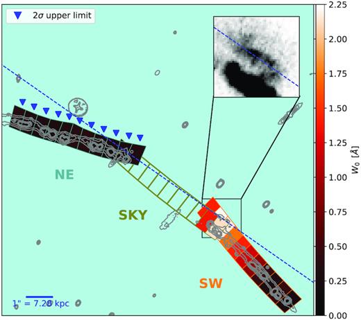
Mg iiW0(2796) map in the absorber (de-lensed) plane. Each spaxel is 3 × 6 kpc2. SKY slit positions with no source illumination are shown transparent. Upper limits (2σ) in the NE slit are indicated with blue triangles). The dashed line indicates the projection of G1’s semimajor axis at PA = 55° N to E. The inset shows an image from the HST F814W band in the absorber plane.
In the following analysis, we consider separately the equivalent widths and the velocities, both as a function of D.
5.2 Equivalent widths versus impact parameter
Fig. 10 summarizes the first of our main results. It shows an anticorrelation between Mg ii λ2796 equivalent width and impact parameter (e.g. Chen et al. 2010; Nielsen et al. 2013b) along the three slit directions used in this work. Thanks to the serendipitous alignment of G1 and the arc segments, this is the first time such a relation can be observed in an individual absorbing galaxy along its major axis.

Mg ii λ2796 rest-frame equivalent width as a function of impact parameter D (in the absorber plane) for SW, NE, and SKY slits. Non-detections are reported as 2σ upper limits. Positions to the north-east of the G1 minor axis are depicted with open symbols. Measurement uncertainties in D (Section 3) come from the astrometry (horizontal error bars) and from the lens model (represented by symbol sizes). For comparison with the quasar statistics, data points from Nielsen et al. (2013b) are displayed (grey symbols). The dashed curve is a scaled version of the isothermal density profile from Chen et al. (2010) using L = 0.14 L* and the shaded region is the RMS of the differences between model and data (see Section 6.2.2 for details).
Noteworthy, there appears to be more coherence towards PSZ1 G311.65–18.48 along the SW slit than in the system studied towards RCS2032727−132623 (Paper I), in the sense that all SW positions have positive detections, having no non-detections down to ≈0.2 Å, our 2σ detection limit. Since we are probing here (1) along the major axis of a disc galaxy and (2) smaller impact parameters, the observed coherence probably indicates that the gas in the disc (this arc) is less clumpy than further away in the halo (RCS2032727−132623).
We compare these arc data with the statistics of quasar absorbers in Section 6.
5.3 Gas velocity versus impact parameter
Fig. 11 displays our second main result. The left-hand panel shows Mg ii–Fe ii absorption velocities in the SW and SKY slits (green and olive colours, respectively) and [O ii] emission velocities (orange colours) as a function of impact parameter, D. The emission velocities come from [O ii] fits in apertures that match SW spaxels #1 to #4 (only the four closest spaxels to G1 show significant [O ii]; Fig. 8). Error bars indicate the uncertainty in the velocity centroid, while the shaded region indicates the projected velocity spread. Note that no spaxel coincides with D = 0 kpc. In this and next figures, we treat impact parameters on the NE side of G1’s minor axis as negative quantities (and hence we get rid of the open symbols). This choice spots apparent rotation around G1 that we discuss below. Given the alignment between the arc and the G1’s major axis, such a plot can be considered a rotation curve. This is the first rotation curve of absorbing gas measured in such a distant galaxy.
![Left-hand panel: Measured line-of-sight velocities versus absorber-plane impact parameter to G1. Green symbols correspond to Mg ii + Fe ii absorption, as measured in the MagE spectra. The green shaded region indicates the projected absorption velocity spread ΔvFWHM at each position. The green dashed curve corresponds to Keplerian fall off from the flat part of the rotation curve. Orange symbols correspond to [O ii] emission, as measured in the MUSE spectra through apertures that match SW spaxels #1 to #4. The orange shaded region corresponds to the projected emission velocity spread ΔvFWHM. The orange dashed curves are rest-frame line-of-sight velocities drawn from the [O ii] emission model at the slit edges shown in the right-hand panel. Distances to the north-east of G1’s semiminor axis have been arbitrarily assign negative values in the impact parameters (see Fig. 6). Impact parameters uncertainties are the same as in Fig. 10. Right-hand panel: Model line-of-sight velocities in km s−1 from z = 0.73379 (Section 4.3). The dashed lines indicate the pseudo-slit used to extract the velocity limits we display in the left-hand panel. The contours correspond to the HST F814W image in the reconstructed absorber plane.](https://oup.silverchair-cdn.com/oup/backfile/Content_public/Journal/mnras/491/3/10.1093_mnras_stz3183/1/m_stz3183fig11.jpeg?Expires=1750258092&Signature=DYU1FtCExWXdncPC8EptNd9FbrFG4~D31622X4xXpQGBij0vtx2~NP9bn9u0rxbs2s-mxDFcoUZXtj2K0qxG1l9dpmAlmAPUj02AzwUC7VS9LbP0dIxh6EhsIjle-BefO4wmrB3JXAc7K1I7zKW1IOzuG6~BVJ8OkBkzCYVwCs585SqYzrDp7FPDAkbg5JYaOW7REm0JPQTNpbaZo76CujCFhaSj67lHZhq15gs44W0wToiDdEh5tbk8Dfsw2a4aktwqtnMI6kyY9qNFgu-BSbei3YOBMJzvU~hQdES~7BzAjr7aVGteZ-RGKk~JoLcTFOpm~BwR1uz1OrrRet4KWw__&Key-Pair-Id=APKAIE5G5CRDK6RD3PGA)
Left-hand panel: Measured line-of-sight velocities versus absorber-plane impact parameter to G1. Green symbols correspond to Mg ii + Fe ii absorption, as measured in the MagE spectra. The green shaded region indicates the projected absorption velocity spread ΔvFWHM at each position. The green dashed curve corresponds to Keplerian fall off from the flat part of the rotation curve. Orange symbols correspond to [O ii] emission, as measured in the MUSE spectra through apertures that match SW spaxels #1 to #4. The orange shaded region corresponds to the projected emission velocity spread ΔvFWHM. The orange dashed curves are rest-frame line-of-sight velocities drawn from the [O ii] emission model at the slit edges shown in the right-hand panel. Distances to the north-east of G1’s semiminor axis have been arbitrarily assign negative values in the impact parameters (see Fig. 6). Impact parameters uncertainties are the same as in Fig. 10. Right-hand panel: Model line-of-sight velocities in km s−1 from z = 0.73379 (Section 4.3). The dashed lines indicate the pseudo-slit used to extract the velocity limits we display in the left-hand panel. The contours correspond to the HST F814W image in the reconstructed absorber plane.
Perhaps the most striking feature in the left-hand panel of Fig. 11 is the decline in velocity at SW spaxels #10 and #11. To explore possible gas rotation, we use our 3D model of [O ii] emission (Section 4.3) and obtain a line-of-sight velocity map at any position near G1 (right-hand panel of Fig. 11). This model might not be unique, but it does serve our purpose of extending it to larger distances for comparison with the absorbing gas. The line-of-sight velocities allowed by the model within an aperture that matches the SW slit are represented in the left-hand panel by the dashed curves. It can be seen that most Mg ii velocities are well comprised by the model velocities, indicating co-rotation of the absorbing gas out to D ≈ 23 kpc. The exception are velocities at SW spaxels #1 (discussed in Section 6.3), and #10 and #11 (Section 6.6).
5.4 Summary of absorption properties
Before proceeding to the discussion, it is useful to consider an overview of the observables by including the other two absorption species detected and their equivalent-width ratios. Such absorption-line summary is shown in Fig. 12, where the upper panel is a simpler version of the left-hand panel in Fig. 11, the middle panel joints equivalent widths of the three species studied in this work, and the bottom panel shows W0 equivalent-width ratios. We concentrate on the standard ratios |$\cal {R}^{\rm Fe\,\small {II}}_{\rm Mg\,\small {II}}$| ≡ W0(2600)/W0(2796) and |$\cal {R}^{\rm Mg\,\small {I}}_{\rm Mg\,\small {II}}$| ≡ W0(2852)/W0(2796), bearing in mind that Mg is an α element and therefore chemical enrichment could affect those ratios.
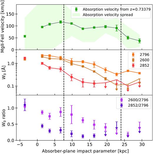
Summary of MagE absorption-line properties at z = 0.73379 towards PSZ1 G311.65–18.48, as a function of impact parameter D from G1. Only SW detections are shown. The only impact parameter to the north-east of G1’s minor axis has been flipped the sign. Upper panel: Velocity of Mg ii + Fe ii line centroids (same as in Fig. 11, left-hand panel). Middle panel: Rest-frame equivalent width of Mg ii λ2796, Fe ii λ2600, and Mg i λ2852. Bottom panel: Equivalent-width ratios. The vertical dashed lines indicate the transitions between the absorption regimes proposed in Section 6.3, i.e. from left to right: disc, disc + inner-halo, and outer-halo absorption.
From the middle panel it can be seen that, like for Mg ii, Fe ii, and Mg i equivalent widths also anticorrelate with D. This is expected, since such species have similar ionization potentials and are most likely co-spatial (Werk et al. 2014).
From the bottom panel of Fig. 12, both |$\cal {R}^{\rm Fe\,\small {II}}_{\rm Mg\,\small {II}}$| and |$\cal {R}^{\rm Mg\,\small {I}}_{\rm Mg\,\small {II}}$| exhibit a general decrease as we probe further out of G1. This is more evident in |$\cal {R}^{\rm Fe\,\small {II}}_{\rm Mg\,\small {II}}$|, which is above 0.5 out to SW#6, and below such threshold beyond. The trend seems real even excluding position SW#1, which is the only measurement above unity (see Section 6.3). In the large-distance end, the two outermost positions have comparatively low |$\cal {R}^{\rm Fe\,\small {II}}_{\rm Mg\,\small {II}}$| values.
6 DISCUSSION
In this section, we synthesize the various observables of G1’s CGM. The discussion revolves around what the observed equivalent widths, kinematics, and equivalent width ratios tell us about the origin of the Mg ii–Fe ii gas. It also highlights the complementarity between our technique and other CGM probes.
6.1 Evolutionary context
G1 seems to be an isolated, sub-luminous (|$0.1L^*_B$|) star-forming (>1.1 M|$\odot$| yr−1) disc-like galaxy. Fig. 7 shows that the [O ii] emission is confined to the optical surroundings, while Mg ii absorption is detected much further out, at least in the direction of the SW slit. This suggests that G1 has recently experienced a burst of star formation, which is detached from the older (and more ordered) cool gas. This is analogous to local galaxies, where H α (also a proxy for star formation) is not necessarily associated with H i (as detected via 21 cm observations, and here considered to be traced by Mg ii), which is usually more extended (Bigiel & Blitz 2012; Rao et al. 2013). Therefore, the offset seen towards PSZ1 G311.65–18.48 should not be surprising for a formed disc still experiencing starbursts, much similar to Mg ii-selected galaxies detected in emission (Bouché et al. 2007; Noterdaeme, Srianand & Mohan 2010).
For comparison with the local Universe, our W0(2796) measurements are ≈3 times higher than those found in M31 (similar halo mass, similar inclination, major axis quasar sightlines) by Rao et al. (2013) at similar impact parameters. Such differences might have an evolutionary or environmental origin, with G1 bearing a larger gaseous content.
6.2 Spatial structure of the CGM
6.2.1 Direct comparison with quasar and galaxy surveys
The grey points in Fig. 10 are drawn from the sample of 182 quasar absorbers in Nielsen et al. (2013b). Note that our data provide seven independent measurements to the sparsely populated interval D < 10 kpc.
In general, our data falls within the quasar scatter, but that scatter is much larger than what we see across the arc. The smaller arc scatter cannot be due only to our particular experimental design. Even if the arc data result from a light-weighted average (over a spaxel area) the spaxels are independent of each other and therefore cannot falsify spatial smoothness on the scales shown in Fig. 10.
In Paper I, we found a similar situation towards RCS2032727−132623. These cases strongly suggest that the scatter in |$W_0^{\rm quasar}$| is not intrinsic to the CGM but rather dominated by the heterogeneous halo population, in which gas extent and smoothness is a function of host–galaxy intrinsic properties (Chen & Tinker 2008; Chen et al. 2010; Nielsen et al. 2013b, 2015; Rubin et al. 2018c) and orientation (Nielsen et al. 2015). It should therefore not be a surprise that quasar-galaxy samples exhibit more scatter than the present case. Furthermore, the same should be true for other extended probes of the CGM like background galaxies (Steidel et al. 2010; Bordoloi et al. 2011; Rubin et al. 2018a,c), which also provide single lines of sight (the exception being the handful of cases where background galaxies resolve foreground haloes; Diamond-Stanic et al. 2016; Péroux et al. 2018).
6.2.2 Isothermal-profile model
We also compare our data with a physically motivated model. The dashed line in Fig. 10 shows a 4-parameter isothermal profile with finite extent, Rgas, developed by Tinker & Chen (2008) to describe |$W_0^{\rm quasar}(D)$|. The isothermal profile was first motivated to model the observed distribution of dynamical mass within ≈30 kpc of nearby galaxies (Burkert 1995). Chen et al. (2010) fitted such a profile to a sample of 47 galaxy–Mg ii pairs and 24 galaxies showing no Mg ii absorption at 10 < D < 120h−1 kpc and obtained the scaling relation Rgas = 74 × (L/L*)0.35 kpc.
We test this model on our arc data by imposing the profile to pass through the W0 value of the closest spaxel to G1 (SW #2). We use L/L* = 0.14 (see Section 4.2) and set the model amplitude to fit W0(2796) = 2.27 ± 0.15 Å at D = 1.4 kpc, leaving the 3 other model parameters in Chen et al. (2010) unchanged. The dashed line in Fig. 10 shows that the isothermal model nicely fits our arc data (RMS = 0.19 Å); moreover, it fits the data not only at the closest spaxel (by construction), but also at almost all impact parameters (excepting the two measurements to the ‘opposite’ side of G1; see next subsection). This is remarkable, since we are fitting a single halo with an isothermal profile that fits the quasar statistics at D > 10 kpc, extrapolated to smaller impact parameters.
The fit has important consequences for our understanding of gaseous haloes. First, it validates an isothermal gas distribution over the popular Navarro–Frenk–White (NFW; Navarro, Frenk & White 1997) profile, which does not predict a flat W0–D relation at small D. This is the first time we can firmly rule out a NFW model for the cool CGM, thanks to our several detections at D < 10 kpc in a single system. Incidentally, the fit also lends support to CGM models that adopt a single density profile (e.g. Stern et al. 2016). Secondly, it suggests that G1’s CGM is representative of the Mg ii-selected absorber population, since it can be modelled with parameters that result from quasar absorber averages and over a wide redshift range. And thirdly, it reveals that the scatter seen in the overall population includes an intrinsic component, likely due to CGM structure on scales of tens of kpc. It seems timely to verify these fundamental points with more measurements at small-D, including single detections towards unresolved background sources.
6.2.3 kpc scales
The overlap of the SKY and SW slits (Fig. 9) helps us to qualitatively assess variations in W0(2796) around G1 on kpc scales. First, SKY positions #10 and #11 partially overlap with SW positions #1 and #2, respectively. The corresponding equivalent widths, though, show no significant differences (see Fig. 10), suggesting that close to G1 (within a few kpc) the gas is smooth on scales of ≈1 kpc, which is roughly the offset between the aforementioned SKY and SW spaxels. This could be due to a covering factor (Steidel et al. 1997; Tripp et al. 2005; Chen & Tinker 2008; Kacprzak et al. 2008; Stern et al. 2016) close to unity at small impact parameters (D ≲ 10 kpc).
6.2.4 Isotropy
The two measurements to the ‘opposite’ side of G1 (i.e. to the north-east of G1; open symbols in Fig. 10) depart by 2–3σ from the trend shown by the SW positions to the south-west of G1 at the same impact parameter (noting that the difference is within the typical scatter reported towards quasar sightlines at larger distances). This indicates that the gas is not homogeneously distributed around G1, even at these small distances.
We are not able to test isotropy of the Mg ii gas on scales between 4 < D < 29 kpc, unfortunately, due to the lack of arc signal right to the north-east of G1. However, NE position #11 is located 29.3 kpc away from G1, just as far as SW position #11 on the other side, and yet it shows no Mg ii down to a stringent 2σ limit of 0.16 Å (log N/cm−2 = 12.7), while the SW position has a significant detection at twice that value. This situation is remarkable, since NE #11 appears in projection on top of the major axis (Fig. 9), while SW #11 lies around 7 kpc away in projection from the same axis. The NE non-detection comes then even more unexpected, under the assumption of isotropy. We conclude that the gas traced by Mg ii, to the extent that we can measure it, is either (1) not isotropically distributed or (2) distributed in a disc which is not aligned with the optical disc or (3) is confined to a (spherical?) volume ≲ 30 kpc in size along G1 major axis. This latter option implies that SW#11 absorption might have an external origin, a possibility we address below.
6.3 Kinematics of the absorbing gas
To the south-west of G1 the absorption signal extends out to ≈8 optical radii along the major axis. Detecting extraplanar gas at z = 0.7 has important consequences for our understanding of disc formation and gas accretion (e.g. Bregman et al. 2018; Stewart et al. 2011a,b). The gas traced by Mg ii shows clear signs of co-rotation (Fig. 11), suggesting that the shape of the rotation curve is not necessarily governed by a combination of outflows in less massive haloes, as we see here a more ordered rotating disc. Our data also confirm the rotation scenario unveiled by simulations (e.g. Stewart et al. 2011b) and also proposed for observations of disc-selected quasar absorbers at z ∼ 1 (e.g. Steidel et al. 2002; Ho et al. 2017; Zabl et al. 2019).
Based on the line centroids at velocity v (left-hand panel in Fig. 11), and excluding the kinematically detached position SW#1 (discussed below), we identify three distinct absorption regimes: (1) disc absorption at D ≲ 10 kpc, where velocities rise to ≈110 km s−1; (2) disc + inner-halo absorption at 10 ≲ D ≲ 20 kpc, where velocities remain flat; and (3) outer-halo absorption at D ≳ 20 kpc, where velocities fall down ‘back’ to v = 0 km s−1.
Interestingly enough, the three proposed regimes correlate with the kinematical complexity of the absorption profiles. In fact, based on the absorption profiles in Fig. 8, the disc absorption corresponds to SW positions #2 to #4, in which ΔvFWHM ≈ 200 km s−1, suggesting several velocity components (also note that position #4 corresponds to the first spaxel beyond the stellar radius; Fig. 5). Then, the disc + halo absorption corresponds to positions #5 to #9, with somewhat simpler absorption kinematics and smaller ΔvFWHM values, suggesting fewer velocity components. We emphasize that we presently cannot resolve individual velocity components and thus v and ΔvFWHM must be considered spectroscopic (and spatial; see Section 3.2) averages.
The dashed lines in the left-hand panel of Fig. 11 show that the two aforementioned regimes are explained, to some extent, by our rotation model. Conversely, SW positions #10 and #11 have the lowest velocity offsets and spreads, and cannot be explained with rotation, even in the Keplerian limit. Such ‘outer-halo’ absorption is one of the most striking signature in the present data, which we discuss in Section 6.6.
Finally, SW #1 also stands out. This position shows a significantly higher velocity offset (∼90 km s−1) than the [O ii] emission, suggesting the dominant absorbing clouds are not tracking the rotation (the same may be also true for part of the SW #2 absorption). The overlapping spaxel SKY #10 shows a consistent velocity, meaning that the measurements are robust. Such kind of offsets are rarely observed in SDSS stacked spectra (Noterdaeme et al. 2010), suggesting their covering factor is low. The arc positions also show the highest |$\cal {R}^{\rm Fe\,\small {II}}_{\rm Mg\,\small {II}}$| values in our sample, which can be explained if the gas is more enriched and processed. These two features conspire in favour of a galactic-scale outflow (Steidel et al. 2010; Kacprzak, Churchill & Nielsen 2012; Shen et al. 2012; Fielding et al. 2017) in one of the velocity components, which is escaping G1 in the line-of-sight direction. Moreover, the spaxels show significant [O ii] flux, and therefore might be co-spatial with star-forming regions, from which supernova-driven winds are expected to be launched (e.g. Fielding et al. 2017; Nelson et al. 2019).
6.4 Gradient in chemical enrichment?
Some of the |$\cal {R}^{\rm Fe\,\small {II}}_{\rm Mg\,\small {II}}$| values in Fig. 12 are exceptionally high compared with the literature (Rodríguez Hidalgo et al. 2012; Joshi et al. 2018). Systems selected in the SDSS by having |$\cal {R}^{\rm Fe\,\small {II}}_{\rm Mg\,\small {II}}$| > 0.5 are found to probe lower impact parameters; moreover, there seems to be a distinction between absorbers associated with high or low SFR depending on whether this ratio is above or below 0.5, respectively (Noterdaeme et al. 2010; Joshi et al. 2018). Our particular experimental setup confirms this trend in the present host galaxy: the four closest positions to G1 show simultaneously the strongest [O ii] emission (Fig. 8) and the highest |$\cal {R}^{\rm Fe\,\small {II}}_{\rm Mg\,\small {II}}$| values (all above 0.5; Fig. 12). Furthermore, |$\cal {R}^{\rm Fe\,\small {II}}_{\rm Mg\,\small {II}}$| seems to show a negative gradient outwards of G1.
Equivalent widths of saturated lines are known to be a function of the number of velocity components (Charlton & Churchill 1998; Churchill et al. 2000), rather than of column density, N. The present spectra do not allow us to resolve such clouds nor to get at their N-ratios, making it hard to assess unambiguously the physical origin of the |$\cal {R}^{\rm Fe\,\small {II}}_{\rm Mg\,\small {II}}$| gradient. Nevertheless, N-ratios must have an effect on |$\cal {R}^{\rm Fe\,\small {II}}_{\rm Mg\,\small {II}}$|. Speculating that both kinematics and line-saturation affect Mg ii λ2796 and Fe iiλ2600 similarly at a fixed impact parameter, a gradient in |$\cal {R}^{\rm Fe\,\small {II}}_{\rm Mg\,\small {II}}$|(D) should globally reflect the same trend in N(Fe ii)/N(Mg ii).
N(Fe ii)/N(Mg ii) is driven by three factors: (a) ionization: but assuming N(H i)≳ 19 cm−2 at D ≲ 20 kpc ≈0.1 Rvir (Werk et al. 2014), ionization is seemingly the less important factor (Giavalisco et al. 2011; Dey et al. 2015); (b) dust: Mg is less depleted than Fe (Vladilo et al. 2011; De Cia et al. 2016); therefore, one expects N(Fe ii)/N(Mg ii) (or |$\cal {R}^{\rm Fe\,\small {II}}_{\rm Mg\,\small {II}}$|) to increase outwards of G1, which we do not observe; and (c) chemical enrichment: α/Fe decreases as Z increases; therefore, N(Fe ii)/N(Mg ii) (|$\cal {R}^{\rm Fe\,\small {II}}_{\rm Mg\,\small {II}}$|) should decrease outwards of G1, which we do observe.
We conclude that we are likely facing the effect of a negative gradient in chemical enrichment, with the outermost positions being less chemically evolved than those more internal to G1. Using high-resolution quasar spectra, in a sample of star-forming galaxies Zahedy et al. (2017) find evidence for a negative gradient in N(Fe ii)/N(Mg ii) as well; however, their ratios fall down (statistically) at larger distances (∼100 kpc) than probed here around a single galaxy. Since Zahedy et al. (2017) galaxy sample is a few to 10 times more luminous than G1, the different scales are likely explained by the luminosity dependence of Rgas (e.g. Chen et al. 2010).
6.5 Damped Lyα systems
Mg ii systems having |$\cal {R}^{\rm Fe\,\small {II}}_{\rm Mg\,\small {II}}$| > 0.5 and W0(2852) > 0.1 Å have been proposed (Rao, Turnshek & Nestor 2006; Rao et al. 2017) to select damped Lyα systems (DLAs; mostly neutral absorption systems having log N(H i) > 20.3 cm−2; e.g. Wolfe, Gawiser & Prochaska 2005) at z < 1.65. According to those criteria, positions SW#1 through #7 classify as DLAs candidates. This lends support to the idea that DLAs occur (at least) in regions internal to galaxies and, furthermore, that some of them are associated with discs both at high and low redshift, as predicted by state-of-the-art simulations (Rhodin et al. 2019). Moreover, the present arc positions classified as DLAs have also the widest velocity dispersions (most of them are within our ‘disc’ kinematical classification), suggesting we are hitting a prototype DLA host (e.g. Ledoux et al. 2006; Neeleman et al. 2013).
Finding DLAs out to 15 kpc (>0.1 Rvir) may be somewhat surprising. Halo models predict columns in excess of the DLA threshold only at very low impact parameters, about three times less than here (Qu & Bregman 2018; but see Mackenzie et al. 2019). The larger extent observed here might be due to the geometrical effect of probing along the major axis of an inclined disc (but see Rao et al. 2013).
Assuming G1 hosts DLA clouds with unity covering factor within a projected disc of radius 15 kpc, we estimate the total mass in neutral gas to be roughly log MHI/M|$\odot$| ≈ 9.5. This is of the order of magnitude of what is found in 21 cm observations at low redshift (e.g. Kanekar et al. 2018), suggesting that G1 represents a high-redshift analogue of a nearby DLA host.
G1’s star formation efficiency, defined as SFR/MH i, is relatively high, SFE = 3.5 × 10⁻¹⁰ yr−1, for the bulk of star-forming galaxies (Popping et al. 2015). On the other hand, the cool gas fraction, defined as MH i/(MH i + M*), falls just below average for z = 0.7: fgas ≈ 0.4 (e.g. Popping et al. 2015). This indicates that G1 is still efficiently forming stars, but will enter a quenching phase – running out of gas in (SFE)−1 ≈ 3 Gyr – if not provided with extra gas supply (Genzel et al. 2010; Leroy et al. 2013; Sánchez Almeida et al. 2014).
6.6 Cold accretion
The Mg ii gas detected at SW positions #10 and #11 stand out in many respects (Fig. 12): it is kinematically detached from the rotation curve; it has larger W0 than an extrapolated trend followed by the more internal positions; and it has the lowest |$\cal {R}^{\rm Fe\,\small {II}}_{\rm Mg\,\small {II}}$| values, likely indicating less processed gas. In addition, spaxel SW #11 lies 7 kpc away in projection from the major axis; depending on the (unknown) disc thickness, the gas detected in these directions could be co-planar and lie at distances of |$\approx 0.2\, R_{\rm vir}$| from G1. These signatures suggest an ‘external’ origin. The absorption profiles at some other SW positions allow for an unresolved velocity component at the velocity of SW #11 (Figs 8 and 11), which could be explained by extended non-rotating gas surrounding the disc. However, such a velocity component would not fit SW #5 through SW #9, nor any of the NE spaxels. We therefore dismiss the surrounding gas scenario for SW #10 and #11. Rather, we consider in-falling gas. Cosmological simulations predict that galaxies hosted by M ≲ 1012 M|$\odot$| haloes should undergo ‘cold-mode’ accretion (e.g. Stewart et al. 2011a). In the following, we consider the possibility to have detected enriched cold accretion at medium redshift (Stewart et al. 2011b; Bouché et al. 2013, 2016; Kacprzak et al. 2014; Danovich et al. 2015; Qu, Bregman & Hodges-Kluck 2019)
Fig. 13 shows a cartoon representation of G1’s inner CGM. The green rotating disc represents the volume where we detect Mg ii–Fe ii–Mg i absorption. The disc is assumed to produce absorption with unity covering factor and to be embedded in a spherical volume likely producing much less covering at our detection limit, W0 > 0.12 Å. This distinction is a possible explanation for the good match with an isothermal model at the SW slit (Fig. 10) and the lack of detections at the NE slit (Fig. 9). In the cartoon model, the extensions of disc and spherical envelope are set arbitrarily such that no absorption is detected to the north-east of spaxel NE #11 (right-most position in the NE slit). Such a choice implies that SW #10 and SW #11 (right-most positions on the SW slit) would not have signal from the disc, but from an external medium, which is consistent with our low-velocity detections. The proposed accreting gas enters the galactic disc radially and roughly transversely to the line of sight (producing the low line-of-sight velocities) while in the process of acquiring enough angular momentum to start co-rotating.

Cartoon model for the inner CGM of the z = 0.7 galaxy studied in this work (G1). The red polygons represent the MagE spaxels, reconstructed in the absorber plane and shown here in the same scale as in Fig. 9. The green rotating disc represents the volume where we detect Mg ii absorption with W0 > 0.12 Å. The disc is centred on the stellar light of G1, has a position angle of 55° N to E, and has an inclination angle of i = 45°, i.e. same parameters as for the stellar disc (see also Fig. 9). The disc is assumed to produce absorption with unity covering factor and to be embedded in a spherical volume producing much less covering at our detection limit. The extensions of disc and spherical envelope are set arbitrarily such that no absorption is detected on spaxel NE #11 (right-most position in the NE slit). The yellow arrow symbolizes in-flowing enriched gas which, if co-planar and aligned with the major axis, would reproduce the observed Mg ii kinematics at SW #10 and SW #11 (left-hand panel in Fig. 11). See Section 6.6 for further discussion.
Alone from the kinematics, though, it is hard to disentangle extraplanar inflow (radial or tangential) from a warped disc (Diamond-Stanic et al. 2016), a scenario that seems to reproduce some observations of quasar absorbers having low line-of-sight velocities (Rahmani et al. 2018; Martin et al. 2019b). Indeed, most of the H i discs in the local Universe exhibit warps (Sancisi et al. 2008; Putman et al. 2009), their extended H i discs do show anomalies (Koribalski et al. 2018), and in a few cases rotation curves start declining when H i becomes patchy in the extended disc of dwarf galaxies (Oikawa & Sofue 2014; Das, Sengupta & Honey 2019). Authors explain such cases via warped and tilted discs (Sofue 2016).
This being said, our data offer enough indications against the warped disc scenario. First, we do not see interacting galaxies (Diamond-Stanic et al. 2016). Secondly, we do not detect absorption at the same distance on the opposite side of G1 (i.e. NE positions #10 and #11). Thirdly, velocities in simulated dwarfs fall down by only 20 per cent at 20 kpc (Oman et al. 2019), while here we see a decline of about |$80{{\ \rm per\ cent}}$|. Indeed, SW positions #10 and #11 have much less specific angular momentum than the rest. For instance SW #11 has 60 per cent less specific angular momentum than SW #10 [i.e. |$(Rv)_{\# 11 }=0.6\times (Rv)_{\#10}$|], and so forth, suggesting the gas is not (yet) rotating. And lastly, the gas shows the lowest |$\cal {R}^{\rm Fe\,\small {II}}_{\rm Mg\,\small {II}}$| values, i.e. it is consistent with less processed gas, which is expected in cold accretion (e.g. Oppenheimer et al. 2012; Kacprzak et al. 2016). Detecting accretion via Mg ii at the level of W0 ∼ 0.2–0.3 Å, although incompatible with pristine gas (Fumagalli et al. 2011; Martin et al. 2019a), agrees well with quasar observations of disc-selected absorbers (Rubin et al. 2012; Zabl et al. 2019).
By averaging spatially the absorption in SW#10 and #11 in a circular aperture of radius 30 kpc, we find that the covering factor is low, faccretion ≈ 1 per cent. This is consistent with simulations at higher redshifts (Faucher-Giguère & Kereš 2011; Fumagalli et al. 2011) and lends support to the cold-accretion scenario.
Altogether, cold, recycled accretion (Rubin et al. 2012; Danovich et al. 2015) at |$\approx 0.2\, R_{\rm vir}$| seems the most favoured scenario to explain the present data. It might be radial accretion at the disc edge (Stewart et al. 2011b; Putman, Peek & Joung 2012) originating from the cool CGM (Werk et al. 2014) in form of recycled winds (Oppenheimer et al. 2010; Anglés-Alcázar et al. 2017), i.e. gas left over from past star-bursts.
This is not the first time absorption kinematics is seen decoupled from emission (Steidel et al. 2002; Ho et al. 2017; Martin et al. 2019b). Velocities below Keplerian have also been detected in quasar sightlines although at slightly larger distances (Ho et al. 2017; Kacprzak 2017; Martin et al. 2019b). Those signatures seem to be frequent in highly inclined discs and authors have argued that they might probe inflows. However, with quasar sightlines probing only one position in the intersected halo, it is challenging to confirm this hypothesis. Thanks to the present tomographic data, we see for the first time a smooth transition to disc co-rotation, providing the first unambiguous evidence for enriched-gas accretion beyond the local Universe.
7 SUMMARY AND CONCLUSIONS
We have studied the cool and enriched CGM of a z = 0.7 star-forming galaxy (G1) via the gravitational arc-tomography technique (Lopez et al. 2018), i.e. using a bright giant gravitational arc as background source. G1 appears to be an isolated and sub-luminous disky galaxy, seen at i ≈ 45°.
We have measured Mg ii, Fe ii, and Mg i equivalent widths (W0) in 25 3 × 6 kpc2 independent positions (including 13 velocity measurements) along G1’s major axis, at impact parameters D = 0–60 kpc (0–0.4 Rvir). This unique configuration has allowed us to probe distinct signatures of the CGM in an individual galactic environment. Our findings can be summarized as follows:
Enriched gas is detected out to D ≈ 30 kpc (≈0.2 Rvir) in one radial direction from G1. The absorption profiles (Fig. 8) show kinematic variations as a function of D, becoming less complex outwards of G1. We suggest that the arc positions probe different regions in the halo and extended disc of G1. Within ∼3 kpc, the smallest scales permitted by our ground-based observations, the gas distribution appears smooth in the central regions (unity covering factor). By comparing W0 measured on both sides of G1, we find evidence that the gas is not distributed isotropically (Fig. 9).
We observe a W0–D anticorrelation in all three studied metal species. The W0(2796) scatter in the arc data (Fig. 10) is significantly smaller than that of the quasar statistics, suggesting biases in the latter, likely due to a variety of host properties and orientations. Our data populates the sparse D < 10 kpc interval, revealing that W0(D) flattens at low impact parameters. An isothermal density profile fits the arc data remarkably well at almost all impact parameters. Since most of the model parameters are tied to the quasar statistics, this suggests that the present halo is prototypical of the Mg ii-selected CGM population. In particular, at D < 10 kpc the good fit rules out cuspy gas distributions, like those described by NFW or power-law models.
For most of the detections, the absorption velocities (Fig. 11, left-hand panel) resemble a flat rotation curve, which appears to be kinematically coupled to G1’s [O ii] emission. There are two exceptions to this trend. (a) One position, lying only 4 kpc in projection from G1 and measured independently in two slits, departs from rotation with a velocity of ∼+90 km s−1. This suggests that the gas, also exhibiting the highest |$\cal {R}^{\rm Fe\,\small {II}}_{\rm Mg\,\small {II}}$| value of the sample, might be out-flowing from G1. (b) The two outer-most detections (at ≈30 kpc ≈0.2 Rvir) also seem decoupled from the disc kinematics, falling too short in velocity. We do not detect absorption at the same distance on the opposite side of G1. We interpret the low-velocity signal as occurring in less-enriched gas having a co-planar trajectory, which will eventually flow into the galaxy’s rotating disc (e.g. an enriched cold-accretion inflow).
The equivalent-width ratio |$\cal {R}^{\rm Fe\,\small {II}}_{\rm Mg\,\small {II}}$|(D) (Fig. 12) exhibits a negative gradient, which could partly be due to a negative gradient in metallicity. This ratio also suggests that G1’s central regions (D < 15 kpc) may host DLAs. We estimate the total reservoir of neutral gas and find it to be comparable with the mass locked into stars, suggesting that the galaxy has little fuel left to keep up with its current star formation efficiency.
8 OUTLOOK
We have highlighted the exquisite advantages of gravitational arc-tomography: (1) the background sources extend over hundreds of kpc2 on the sky, permitting a true ‘slicing’ of the CGM of individual intervening galaxies; (2) comparison with the statistics of quasar-galaxy pairs offers a great opportunity to assess the gas patchiness and its covering factor around individual systems, something beyond the capabilities of present-day quasar observations; (3) the individual systems can be used as test laboratories in future simulations. Challenges are manifold as well: sensitive spatially resolved spectroscopy is needed (not available until recently); absorber-plane reconstruction is required via ad hoc modelling of the lensing configuration (usually non-trivial); bright giant gravitational arcs are rare on the sky. We expect that soon new surveys will provide targets for future extremely large observing facilities. In the meantime, a comparison scheme between the arc and quasar statistics can and must be developed. These are key aspects that nicely complement quasar studies. Furthermore, with higher spectral resolution one shall be able to resolve individual velocity components and assess the chemical state of the gas in a spatial/kinematical context. Undoubtedly, such tools shall enable a more profound understanding of the baryon cycle across galaxy evolution.
ACKNOWLEDGEMENTS
We thank the anonymous referee for comments that improved the manuscript. This work has benefited from discussions with Nikki Nielsen, Kate Rubin, Glenn Kacprzak, Umberto Rescigno, and Nicolas Bouché. This paper includes data gathered with the 6.5 m Magellan Telescopes located at Las Campanas Observatory, Chile: the Magellan/MagE observations were carried out as part of program CN2017B-57 (PI Tejos). The VLT/MUSE data were obtained from the ESO public archive [program 297.A-5012(A), PI Aghanim]. This work was supported in part by NASA through a grant (HST-GO-15377.01, PI Bayliss) awarded by the Space Telescope Science Institute, which is operated by the Association of Universities for Research in Astronomy, Inc. under NASA contract NAS 5-26555. SL was partially funded by UCh/VID project ENL18/18 and by FONDECYT grant number 1191232. NT acknowledges support from PUCV/VRIEA projects 039.333/2018 and 039.395/2019, and FONDECYT grant number 1191232. LFB was partially supported by CONICYT Project BASAL AFB-170002. MG was supported by NASA through the NASA Hubble Fellowship grant #HST-HF2-51409 awarded by the Space Telescope Science Institute, which is operated by the Association of Universities for Research in Astronomy, Inc., for NASA, under contract NAS5-26555.
Footnotes
The [C iii] emission line of the source is useful in this context because it appears as several unresolved knots at different relative positions along each arc segment.
REFERENCES
APPENDIX A: MAGELLAN/MagE DATA
A1 Magellan/MagE data acquisition
We observed the two northernmost segments in PSZ1 G311.65–18.48 with Magellan/MagE (Marshall et al. 2008) in dark-time on 2017 July 20 and 21 (both first half-nights). Given the large declination of the field the observations were conducted with airmass restricted between 1.55 and 1.66. The seeing was good and steady on both half-nights, varying between 0.6 and 0.7 arcsec. However, the general weather conditions varied between the two half-nights, being cloudy (cirrus) during most of the first half-night and clear on the second. This situation affected the quality of some of the exposures taken during the first half-night, from which only one exposure of the SW slit was finally used. On the other hand, we used all exposures taken for the NE, SW, and SKY slits on the second half-night. Table 1 gives a summary of the useful observations.
Data acquisition was performed from blind offsets with respect to a nearby bright star located at Celestial Coordinate (J2000) RA = 15h50m00s and Dec. = −78°10m57s. Because our PAs are different than the Parallactic Angle at a given time (72°, 42°, and 52.3°, for ‘NE’, ‘SW’, and ‘SKY’, respectively), we used a blue filter in the acquisition camera; in this manner, we ensure that the bluest possible optical coverage of the arcs (where the transitions of interest fall), were correctly aligned within the slits.
Individual exposure times varied between |$2\, 700$| and |$4\, 500$| s, for a total of 2.0, 3.0, and 1.17 h for slits ‘NE’, ‘SW’, and ‘SKY’, respectively, as presented in Table 1.
A2 Magellan/MagE data reduction
We used a custom pipeline to reduce the MagE data. Because we deal here with an extended source, the main task is to account for the known misalignment between the spatial direction and the CCD columns on the two-dimensional (2D) spectra, a tilt which varies with position on the CCD (e.g. Bochanski et al. 2009). To this end, for each 2D spectrum we define 33 one-pixel (0.3 arcsec) long pseudo-slits, whose positions correspond to an offset with respect to the previously defined Echelle orders, and for each pseudo-slit we obtain independent wavelength solutions. Variance frames are created from the 2D spectra of each object, and cosmic rays are assigned with ‘infinite’ variances.
We extract and reduce the flux and the variance at each pseudo-slit by linearly interpolating the values in the image, order by order. A master sky spectrum is obtained from the slit ‘SKY’ by averaging spatially 20 pseudo-slits in the central part of the slit (the slit extremes have flux from the arc segments by design). A scaled version of the master sky is subtracted equally to the flux at all pseudo-slits in a given exposure, with scale factors chosen in such a way that SW positions #2, #3, and #4 (all having black absorption) end up with no residuals above the zero flux level.
A response function is created by reducing a spectrophotometric standard. Division of the object spectra by this function converts the sky-subtracted counts into flux units and corrects the blaze function of the spectrograph. The orders are merged into a one-dimensional, calibrated and reduced spectrum. Finally, wavelengths are corrected for barycentric velocities and the different exposures co-added optimally by weighting by the inverse variances.
As a compromise between matching the seeing and maximizing S/N, for each of the ‘NE’, ‘SKY’, and ‘SW’ slits, we combine the 33 pseudo-slit spectra along three consecutive offsets (Fig. 3). This spatial binning defines 11 ‘pseudo-spaxels’ on the plane of the sky (referred to as ‘MagE spaxels’ or ‘positions’) of 0.9 arcsec × 1.0 arcsec each, oriented along the slits (Fig. 1, Fig. 2 and subsequent figures). Each spaxel is separated by ≳1 seeing units from the next, ensuring that the signals are mostly independent. Due to the inhomogeneous source brightness along the slit (and not due to partial source illumination; see Fig. 2), the spectra have different S/N, ranging typically from 4 to 10.
The final resolving power, as measured from sky emission lines, is |$R=4\, 500$| with a dispersion of 0.37183 Å pix−1 (or ≈22 km s−1 at the position of Mg ii) and an RMS of ≈0.06 Å. This RMS is similar to that reported by Bochanski et al. (2009). To check the wavelength calibration, we select sky lines in the MagE and in the MUSE data (see Section 2.2) and calculate their centroids. An histogram of velocity differences appears centred around zero with a dispersion of σ = 12 km s−1; therefore, these reduced MagE spectra can be compared with the MUSE spectra. As a sanity check, we inspected the match with the sky line at λ = 4861.32 Å (this is right at the position of the expected Mg ii absorption; Fig. 3) and found them to be consistent.
Finally, the combined spectra for a given slit were recorded into data-cubes of a rectangular shape of 1 × 11 spaxels. Throughout the paper we use the convention that the northernmost spaxel in a given slit is ‘position 1’ (#1) and these increase towards the South in a consecutive order, being the ‘position 11’ (#11) the southernmost spaxel in a given MagE slit (e.g. ‘SW #1, #2, #3, etc.; see Figs 1 to 3).
A3 Magellan/MagE astrometry
Although the slit acquisition was executed by a blind offset from a reference source, the process of acquiring the reference star was performed manually (by the telescope operator) and may introduce a small position offset of a fraction of an arcsecond. To make sure that the astrometry of our MagE slit data-cubes matches to that of MUSE (and hence HST; see Section 2.2), we proceed as follows.
First, we used the MUSE data-cubes as reference to create several mock MagE data-cubes from the MUSE data (referred to as ‘MUSE-MagE’) using the pymuse package (Pessa, Tejos & Moya 2018). Each MUSE-MagE data-cube has 11 spaxels with the exact geometry of our MagE slits, placed at a fixed PA (given by the corresponding MagE slit) but with a different central position. As we made sure the arcs segments were well within the slits, we only varied the slits positions over ±1 arcsecalong their corresponding PA directions.
For each of the resulting MUSE-MagE data-cubes, we compared the spectral shape and total flux per spaxel to those of the actual corresponding MagE data-cube (rebinned to the coarser wavelength dispersion of MUSE) within the wavelength range between 6420 and 6440 Å, i.e. encompassing the [C iii] λλ1907, 1909 emission line of the arc source.2 We computed a spectral and a total flux (per spaxel) χ2 for the different mock MUSE-MagE data-cubes and adopted the position that minimized it as our astrometry solution (as presented in Fig. 1). From the shape of the χ2 curves around the minimum we estimate a position uncertainty of the MagE slits of 0.2 arcsec. We note that this is a systematic uncertainty that applies to all MagE spaxels in the same direction for a given MagE slit.
APPENDIX B: MORPHOKINEMATICAL ANALYSIS OF G1 FROM [O ii] EMISSION
We performed a morphokinematical analysis of G1 using the galpak software (v.1.11; Bouché et al. 2015), from which we fit a rotating disc model to the [O ii] emission observed in the MUSE datacube. First, we created a de-lensed MUSE datacube at the absorber plane, centred around G1. We re-sampled the resulting smaller de-lensed spaxels into the MUSE pixel scale of 0.2 arcsec pixel−1, thus preserving the original geometry. The input instrument line-spread function was that of MUSE (FWHM = 2.675 Å), and the input PSF was the effective reconstructed (elongated) seeing PSF at the absorber plane.
We run galpak on the continuum-subtracted and de-lensed datacube around the [O ii] emission (centred around G1), for |$10\, 000$| iterations until convergence for a disc model with the following parameters: an exponential flux profile, an arctan rotation curve, and a Gaussian thickness profile. Although the [O ii] flux profile was not properly modelled as a single disc component (some significant residuals are present due to the presence of clumpy star formation regions), the model did converge to a satisfactory kinematical solution whose main parameters are presented in Table 2. We finally estimated a virial radius, Rvir, and a dynamical halo mass, |$M_\mathrm{ h}^{\rm dyn}$|, assuming a spherical collapse model as Rvir = 0.1H(z)−1vmax, and |$M_{\rm dyn}= 0.1 H(z)^{-1}G^{-1}v_{\rm max}^3$|, where H(z) is the Hubble parameter at redshift z and G is the gravitational constant (Mo, Mao & White 1998; Rahmani et al. 2018, see Table 2).
APPENDIX C: FITTED ABSORPTION-LINE PROFILES

Transitions detected in SW positions #1 through #4. The histograms show the normalized flux and its 1σ error. The red curves are the fitted Voigt profiles.

Same as Fig. C1 for SW positions #5 through #8.
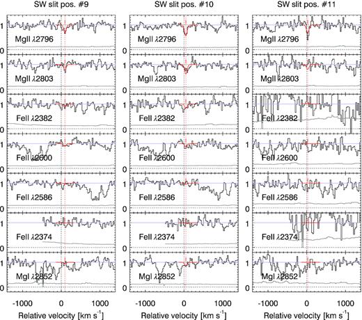
Same as Fig. C1 for SW positions #9, #10, and #11.

Same as Fig. C1 for SKY positions #1, #10, and #11.

Same as Fig. C1 for NE positions #1 through #4.

Same as Fig. C1 for NE positions #5 through #8.
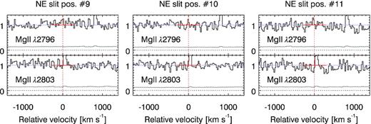
Same as Fig. C1 for NE positions #9, #10, and #11.
