


ABSTRACT
We present simulations of galaxy formation, based on the gadget-3 code, in which a sub-resolution model for star formation and stellar feedback is interfaced with a new model for active galactic nucleus (AGN) feedback. Our sub-resolution model describes a multiphase interstellar medium (ISM), accounting for hot and cold gas within the same resolution element: we exploit this feature to investigate the impact of coupling AGN feedback energy to the different phases of the ISM over cosmic time. Our fiducial model considers that AGN feedback energy coupling is driven by the covering factors of the hot and cold phases. We perform a suite of cosmological hydrodynamical simulations of disc galaxies (|$M_{\rm halo,DM} \simeq 2 \times 10^{12}$| M⊙, at z = 0), to investigate: (i) the effect of different ways of coupling AGN feedback energy to the multiphase ISM; (ii) the impact of different prescriptions for gas accretion (i.e. only cold gas, both cold and hot gas, with the additional possibility of limiting gas accretion from cold gas with high angular momentum); (iii) how different models of gas accretion and coupling of AGN feedback energy affect the coevolution of supermassive black holes (BHs) and their host galaxy. We find that at least a share of the AGN feedback energy has to couple with the diffuse gas, in order to avoid an excessive growth of the BH mass. When the BH only accretes cold gas, it experiences a growth that is faster than in the case in which both cold and hot gas are accreted. If the accretion of cold gas with high angular momentum is reduced, the BH mass growth is delayed, the BH mass at z = 0 is reduced by up to an order of magnitude, and the BH is prevented from accreting below z ≲ 2, when the galaxy disc forms.
1 INTRODUCTION
AGN (active galactic nucleus) activity is observed across cosmic time, and the role of AGN feedback is fundamental in regulating the formation and evolution of galaxies. The existence of tight correlations between properties of SMBHs (supermassive black holes) and their host galaxies (or better, their host galaxy bulges – e.g. Magorrian et al. 1998; Ferrarese & Merritt 2000; Gebhardt et al. 2000; Merritt & Ferrarese 2001; Tremaine et al. 2002; Marconi & Hunt 2003; Häring & Rix 2004; Gaspari et al. 2019) is commonly interpreted as the evidence of a coevolution of BHs and host galaxies. According to this scenario, the host galaxy evolution and the physical properties of its interstellar medium (ISM) regulate BH feeding and growth; conversely, feedback from BHs determines and shapes general properties of the host galaxy. However, there is no general consensus on the scenario of BH-galaxy coevolution and SMBH self-regulation: rather, observed scaling relations could be explained as the result of common mechanisms (e.g. mergers and/or gas accretion) which drive the formation of both SMBHs and their host galaxies (e.g. Croton et al. 2006; Alexander & Hickox 2012; Dekel, Lapiner & Dubois 2019). Hydrodynamical simulations that model structure formation and evolution in a cosmological context have to take into account the effect of AGNs. Indeed, nuclear galactic activity is deemed fundamental to simulate structures whose properties are in agreement with observations at different redshifts.
In particular, the role of AGN feedback is key in controlling the star formation and the gas cooling processes in galaxies. AGNs can have both a positive (e.g. Silk 2013; Bieri et al. 2015; Cresci et al. 2015a; Wagner et al. 2016; Cresci & Maiolino 2018) and a negative (e.g. Croton et al. 2006; McNamara & Nulsen 2007; Fabian 2012; Wylezalek & Zakamska 2016) impact on the star formation of their hosts. They can stimulate some degree of cooling, enhancing the star formation (the so-called positive feedback), or they can produce an overall heating and/or mechanical ejection of the gas from the central regions of the galaxy, ultimately quenching the star formation (Lapi et al. 2006, 2014, 2018; Peterson & Fabian 2006; Cresci et al. 2015b; Carniani et al. 2016; McNamara et al. 2016). The relative importance of these processes is still under debate.
In recent years, a wealth of multiwavelength observations has revealed the presence of gas spanning a wide range of densities, temperatures, and ionization states in and around galaxies. This multiphase gas is ubiquitous not only in spiral galaxies, commonly recognized as systems rich in cold gas, but also in ellipticals and in the innermost regions of galaxy groups and clusters, environments commonly known to be dominated by X-ray emitting hot gas (e.g. David et al. 2014; Werner et al. 2014). This multiphase component has been observed to be present also in galactic-scale outflows, which represent one of the most characteristic imprints of the AGN presence in a system (e.g. Chartas, Brandt & Gallagher 2003; Rupke & Veilleux 2011; Cicone et al. 2014; Feruglio et al. 2015; Tombesi et al. 2015; Morganti et al. 2016; Russell et al. 2019).
Multiphase outflows powered by AGNs are a direct consequence of the fact that the energy generated by the accreting SMBH is coupled to the surrounding ISM in what is commonly referred to as AGN feedback. It is still debated how cold gas gets involved into galactic scale outflows, if by outward acceleration of cold gas already present in the innermost regions of the host system, or by condensation of outflowing hot gas, resulting in a cold outflow. These possibilities have been considered both by observational (e.g. Alatalo et al. 2011; Combes et al. 2013; Morganti et al. 2013; Russell et al. 2014) and numerical (e.g. Gaspari, Brighenti & Temi 2012b; Li & Bryan 2014; Costa, Sijacki & Haehnelt 2015; Valentini & Brighenti 2015) studies. Whatever the origin of the cold outflowing gas, observed cold and molecular outflows are thought to be mainly accelerated directly by the AGN, as it is unlikely that cold gas has been induced to outflow by entrainment by the hot gas phase outflow. As a consequence, the AGN feedback energy has to be transferred to both the diffuse and cold phases. This complex process is still far from being fully understood, and thus an accurate modelling in cosmological hydrodynamical simulations is still missing.
SMBHs accrete surrounding gas and the released gravitational energy provides feedback energy. AGN feedback develops through the interaction between the mechanical, thermal, and radiative energy supplied by accretion and the gas in the host galaxy. BH feedback operates through two main distinct modes (although this distinction is purely phenomenological and conventional): quasar (or radiative) mode, and radio (or kinetic) mode (e.g. Fabian 2012). During the quasar mode the AGN is highly luminous, its luminosity approaching the Eddington limit, i.e. LEdd ≃ 1.3 × 1038 (MBH/M⊙) erg s−1 (Frank, King & Raine 2002). Quasar radiation likely originates from an accretion disc; at large scales, gas-rich mergers and cold flows are supposed to be the main mechanisms by which the BH is fed during this phase, as they can sustain high BH accretion rates. Feedback energy is released through winds and by radiation when AGNs are in quasar-mode. On the other hand, the accreting BH acts through the mechanical energy of its radio-emitting jets during the radio mode. These collimated jets can inflate cavities and bubbles in the hot atmosphere of dark matter (DM) haloes, and entrain ambient gas resulting in massive outflows, that are sub-relativistic on kpc scales. The latter mode is dominant among low-power AGNs at redshift z ≲ 2 (unless we consider Seyfert galaxies), where BHs are characterized by lower accretion rates and mainly sustained by the secular evolution of the host system (e.g. reviews by Ferrarese & Ford 2005; McNamara & Nulsen 2007; Fabian 2012; Kormendy & Ho 2013; Morganti 2017, and references therein). Radiation pressure can also power outflows (Proga 2007). AGN feedback energy also affects the accretion and growth of the BH itself, thus controlling its duty-cycle and making the system reach the self-regulation.
A key point that is under debate is the best way to capture an effective description of AGN feeding and feedback in cosmological simulations. Sub-resolution prescriptions adopted to simulate both the mechanism through which the gas is accreted on to the SMBH and the way of releasing energy are burning issues. As for AGN feedback, the commonly pursued approaches consist in providing the feedback energy to the surrounding medium in the form of thermal or kinetic energy (e.g. Springel, Di Matteo & Hernquist 2005; Sijacki et al. 2007; Dubois et al. 2010; Barai et al. 2016), or with a combination of the two (Davé et al. 2019). The recently pursued direction of investigation aims at simulating the effect of the radiative power of the AGN via the injection of thermal energy, while modelling the outcome of the mechanical power of the AGN by means of outflows in the form of kinetic feedback (e.g. Steinborn et al. 2015; Weinberger et al. 2017, and references therein).
As for AGN feeding, the most common way to model gas accretion on to SMBHs is to assume the Bondi accretion (see Section 3.2 for details). However, due to the inability of resolving the Bondi radius in cosmological hydrodynamical simulations, the estimate of the Bondi accretion needs to be done by sampling gas properties over quite large volumes in the proximity of the BH. Indeed, in order to properly represent the Bondi accretion, one has to resolve the Bondi radius |$r_{\rm B} = G\, M_{\rm BH} / c_{\rm s}^2 \sim 0.04(M_{\rm BH}/10^6 \, \text{M}_{\odot }) \, (c_{\rm s}/ 10 \, \text{km s}^{-1})^{-2}$| kpc, where G, MBH, and cs are the gravitational constant, the BH mass, and the sound speed of the ambient gas, respectively (Edgar 2004; Booth & Schaye 2009); on the other hand, cosmological simulations generally have spatial resolutions spanning from few kpc down to few hundreds of pc (for instance, simulations in this paper have a force resolution which is from two to three orders of magnitude larger than the typical Bondi radius of BHs in our galaxies). This lack of resolution causes gas density to be underestimated, while gas temperature is overestimated. This leads to an underestimation of the accretion rate, that is commonly boosted in order to have an effective AGN feedback and to match the observations (Di Matteo, Springel & Hernquist 2005; Booth & Schaye 2009; Negri & Volonteri 2017). To overcome this limitation, challenging mass-refinement techniques (Curtis & Sijacki 2015; Beckmann, Devriendt & Slyz 2019) have been recently developed to increase resolution in the BH surroundings, but till now they have been employed in simulations of isolated galaxies only. Moreover, cold gas that accretes on to SMBHs is expected to deviate considerably from the idealized Bondi assumptions (e.g. Gaspari, Ruszkowski & Oh 2013, and Section 3.3).
The properties of the ISM surrounding SMBHs in the centre of galaxies, galaxy groups and clusters are thought to regulate the BH feeding. Also, the presence of a multiphase medium in the innermost regions of cosmic structures poses a challenging question: how different gas phases experience AGN feedback?
The key questions that we want to address in this Paper are the following: how do accreting BHs transfer feedback energy to the surrounding multiphase ISM? How do they determine the properties of their host galaxy? How do different models and regimes of gas accretion affect the BH-galaxy coevolution? Does AGN feedback affect significantly the circulation of heavy elements within the galaxy?
The sub-resolution model MUPPI (MUlti Phase Particle Integrator; Murante et al. 2010, 2015) that we adopt for our cosmological simulations of galaxy formation is crucial to carry out this investigation. Indeed, it describes a multiphase ISM (Section 2) and solves the set of equations accounting for mass and energy flows among the different phases within the SPH time-step itself: these features are key to explicitly and effectively model the effect of AGN feedback energy within the resolution element (i.e. the multiphase gas particle).
This paper is organized as follows. Section 2 describes the main features of the original sub-resolution model MUPPI. Section 3 is devoted to introduce the AGN feedback model that we implemented within the code and the sub-resolution model adopted for cosmological simulations. In Section 4, we introduce the suite of simulations that we carried out, and in Section 5 we present and discuss results. The main conclusions are drawn in Section 6.
AGNs operate in systems with different mass residing in different environments, from isolate spiral galaxies to massive ellipticals located at the centre of bright groups and clusters of galaxies. This work is focused on late-type galaxies: we introduce our AGN feedback model and explore how it works within the scenario of disc galaxy formation and evolution. The investigation of the effect of AGN feedback in elliptical galaxies is postponed to a forthcoming work.
2 THE SUB-RESOLUTION MODEL: STAR FORMATION AND STELLAR FEEDBACK IN A MULTIPHASE ISM
In this sction, we outline the most relevant features of the model, while a more comprehensive description and further details can be found in the introductory papers by Murante et al. (2010, 2015).
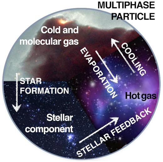
Cartoon showing the composition of a multiphase gas particle within the MUPPI model. Mass and energy flows among different components are highlighted with arrows.
Relevant parameters of the sub-resolution model.
| nthresh | Tc | P0 | Pkin | twind | θ | ffb,therm | ffb,kin | ffb,local | fev | f* | N* | |$M_{\ast , \rm SN}$| |
|---|---|---|---|---|---|---|---|---|---|---|---|---|
| (cm−3) | (K) | (kB K cm−3) | (Myr) | (°) | (M⊙) | |||||||
| 0.01 | 300 | 2 × 10⁴ | 0.05 | 15 – |$t_{\rm dyn, c\, [Myr]}$| | 30 | 0.2 | 0.26 | 0.02 | 0.1 | 0.02 | 4 | 120 |
Note. Column 1: number density threshold for multiphase particles. Column 2: temperature of the cold phase. Column 3: pressure at which the molecular fraction is fmol = 0.5. Column 4: gas particle’s probability of becoming a wind particle. Column 5: maximum lifetime of a wind particle. Columns 6: half-opening angle of the cone for thermal feedback, in degrees. Columns 7 and 8: thermal and kinetic SN feedback energy efficiencies, respectively. Column 9: fraction of SN energy directly injected into the hot phase of the ISM. Column 10: evaporation fraction. Column 11: star formation efficiency, as a fraction of the molecular gas. Column 12: number of stellar generations, i.e. number of star particles generated by each gas particle. Column 13: average stellar masses of stars formed per each SN II.
The second source term is |$\dot{E}_{\rm hydro}$|: it accounts for the energy contributed by neighbour particles because of thermal feedback from dying massive stars (see below), and also considers shocks and heating or cooling due to gravitational compression or expansion of gas.
A gas particle exits its multiphase stage after a maximum allowed time given by the dynamical time of the cold gas (tdyn,c). When a gas particle exits a multiphase stage, it has a probability Pkin of being kicked and to become a wind particle for a time interval twind. Both Pkin and twind are parameters of the model (Table 1). This scheme relies on the physical idea that galactic winds are powered by SN II explosions, once the molecular cloud out of which stars formed has been destroyed. Wind particles are decoupled from the surrounding medium for the aforementioned interval twind. During this time, they receive kinetic energy from neighbouring star-forming gas particles. The wind stage can be concluded before twind whenever the particle density drops below a chosen density threshold, |$0.3 \, \rho _{\rm thresh}$|, meaning that a wind particle has finally gone away from star-forming regions. We note that a multiphase particle is forced to exit the multiphase stage if its density drops below |$0.2 \, \rho _{\rm thresh}$|, as star formation is not expected to occur anymore in the ISM that it samples.
The system of equations (4), (5), (6), and (7) is integrated with a Runge–Kutta algorithm within each SPH time-step (see Murante et al. 2010, 2015, for details).
The original release of the sub-resolution model MUPPI does not include the effect of AGN feedback. In Section 3, we introduce the implementation of AGN feedback within our sub-resolution model.
2.1 Additional physics: cooling and chemical enrichment
Chemical enrichment and radiative cooling are self-consistently included in our simulations. Metal-dependent radiative cooling is implemented according to the model by Wiersma, Schaye & Smith (2009a). Cooling rates are estimated on an element-by-element basis, by adopting pre-computed tables where rates are functions of density, temperature, and redshift. Tables have been compiled using the spectral synthesis code cloudy (Ferland et al. 1998). The gas is considered to be optically thin and exposed to a spatially uniform, redshift-dependent ionizing background radiation from star-forming galaxies and quasars (Haardt & Madau 2001). When computing cooling rates, photoionization equilibrium is thus assumed (see Wiersma et al. 2009a,b, for details).
Besides providing the ISM with energy, stellar feedback resulting from star formation and evolution also supplies heavy elements (chemical feedback), and galactic outflows foster metal spread and circulation throughout the galaxy. Our model self-consistently accounts for the chemical evolution and enrichment processes, following Tornatore et al. (2007), where a thorough description can be found. Here, we only highlight the most crucial features of the model.
The model accounts for different time-scales of evolving stars with different masses by adopting the mass-dependent lifetimes by Padovani & Matteucci (1993). The minimum mass giving rise to stellar BHs is considered to be 8 M⊙. Stars that are more massive than 40 M⊙ directly implode into BHs, thus not contributing to further chemical enrichment nor to stellar feedback.
A fraction of stars relative to the entire mass range in which the IMF is defined (see Section 4) is assumed to be located in binary systems suitable for being progenitors of SNe Ia. It is set to 0.03: the effect of the value of this fraction is extensively explored in Valentini et al. (2019). Energy contributed by SNe Ia which is provided to multiphase particles enters in the source term |$\dot{E}_{\rm hydro}$| in equation (7).
The production of different metals by aging and exploding stars is followed by assuming sets of stellar yields. We adopt the stellar yields provided by Thielemann et al. (2003) for SNe Ia and the mass- and metallicity-dependent yields by Karakas (2010) for intermediate and low mass stars that undergo the AGB (asymptotic giant branch) phase. As for SNe II, I use the mass- and metallicity-dependent yields by Woosley & Weaver (1995), combined with those provided by Romano et al. (2010). Also, the effect of adopted stellar yields is addressed in detail in Valentini et al. (2019).
Different heavy elements produced and released by star particles are distributed to neighbouring gas particles with kernel-weighted contributions, so that subsequently generated star particles are richer in metals. The chemical evolution process is therefore responsible for the gradual reduction of the initial mass of stellar particles, too. We follow in detail the chemical evolution of 15 elements (H, He, C, N, O, Ne, Na, Mg, Al, Si, S, Ar, Ca, Fe, and Ni) produced by different sources, namely AGB stars, SNe Ia, and SNe II. Each atomic species independently contributes to the cooling rate, as discussed above.
Note that the mass of gas particles is not constant throughout the simulation: the initial mass can indeed decrease due to star formation (i.e. spawning of star particles), and it can increase because of gas return by neighbour star particles.
3 AGN FEEDBACK MODELLING
In this section, we describe the AGN feedback model adopted to carry out the simulations presented in this paper. BH accretion and ensuing feedback are modelled resorting to sub-resolution prescriptions, as for star formation and stellar feedback (see Section 2). The prescriptions adopted for BH seeding and accretion are predominantly based, despite a number of differences that are detailed in the following, on the original model by Springel et al. (2005) and largely inherited from simulations of galaxy clusters (e.g. Fabjan et al. 2010; Ragone-Figueroa et al. 2013; Rasia et al. 2015; Steinborn et al. 2015). As for the modelling of the release of AGN feedback energy, since the sub-resolution model MUPPI describes a multiphase ISM, we exploit this feature in order to study the coupling of AGN feedback energy to different phases of the ISM (by modelling the energy distribution within multiphase particles).
3.1 Including BHs: seeding and pinning
BHs in cosmological hydrodynamical simulations are represented by means of collisionless sink particles of mass MBH. BH particles are introduced in massive haloes at relatively high redshift in cosmological simulations, and they are then allowed to grow and increase their initial or seed mass. As we are still lacking a solid understanding of the formation of first SMBHs (see e.g. Bromm & Loeb 2003; Begelman, Volonteri & Rees 2006; Mayer et al. 2010; Volonteri & Bellovary 2012; Maio et al. 2019, for possible scenarios), BHs are first inserted according to seeding prescriptions.
In the simulations presented in this section, a BH of theoretical mass |$M_{\rm BH,seed}$| is seeded within DM haloes whose mass exceeds the threshold mass MDM,thresh, and that do not already have a BH. The commonly quoted mass MBH is the theoretical mass of the BH, modelled at the sub-resolution level; its dynamical mass is the actual gravitational mass of the BH particle in the simulation (the two masses are in general not equal, see Section 3.2). We adopt |$M_{\rm BH,seed}=1.1 \times 10^5$| M⊙ and MDM,thresh = 1.7 × 10¹⁰ M⊙ for the fiducial simulations (see Table 2 and Section 4). We exploited the Mbulge–MBH relation to choose the reference |$M_{\rm BH,seed}$| (see Appendix B). Also, the eligible DM halo is required to have a minimum stellar mass fraction (|$f_{\rm \star ,seed} = 0.02$|) for BH seeding. The latter requirement ensures that BHs are seeded only within haloes that host adequately resolved galaxies (Hirschmann et al. 2014).
Relevant parameters of the AGN model.
| |$M_{\rm BH,seed}$| | |$M_{\rm DM,thresh}$| | |$f_{\rm \star ,seed}$| | Tsplit | ϵr | ϵf | Cvisc |
|---|---|---|---|---|---|---|
| (M⊙) | (M⊙) | (K) | ||||
| 1.1 × 10⁵ | 1.7 × 10¹⁰ | 0.02 | 5 × 10⁵ | 0.1 | 0.01 | |$2 \, \pi \times (1,10^2,{\text{or }} 10^3)$| |
| |$M_{\rm BH,seed}$| | |$M_{\rm DM,thresh}$| | |$f_{\rm \star ,seed}$| | Tsplit | ϵr | ϵf | Cvisc |
|---|---|---|---|---|---|---|
| (M⊙) | (M⊙) | (K) | ||||
| 1.1 × 10⁵ | 1.7 × 10¹⁰ | 0.02 | 5 × 10⁵ | 0.1 | 0.01 | |$2 \, \pi \times (1,10^2,{\text{or }} 10^3)$| |
Note. Column 1: BH seed mass in the reference simulations. Column 2: halo mass for BH seeding. Column 3: minimum stellar mass fraction for BH seeding. Column 4: threshold temperature to distinguish between hot and cold accreting gas. Column 5: radiative efficiency. Column 6: feedback efficiency. Column 7: reference value for the parameter regulating the angular momentum dependent accretion of cold gas.
DM haloes are identified by means of the Friends-of-Friends (FoF) algorithm. The FoF is performed on-the-fly, on DM particles alone, and a linking length of 0.16 times the mean inter-particle spacing is adopted. To achieve an accurate centring of the BH particle in the pinpointed halo, the BH is seeded in the position of the minimum potential of the halo, by identifying the star particle which has the highest binding energy. The selected star particle is thus converted into a BH sink particle of theoretical mass |$M_{\rm BH,seed}$|. The dynamical mass of the BH at the seeding is the mass of the star particle which has been converted into it. The initial mass of gas particles can be thus considered as a typical dynamical mass of a seed BH.
The location of the BH is crucial to determine physical properties of the gas that undergoes accretion and to compute quantities involved in the ensuing feedback. In simulations, BHs can generally move away from the innermost regions of the forming galaxy and wander because of numerical artefacts (Wurster & Thacker 2013): indeed, they can be dragged by surrounding particles, especially in highly dynamical, high-redshift environments. Also, the dynamical friction that is expected to promote the settling of massive BHs in the centre of haloes usually is not adequately captured at the resolution achieved in cosmological simulations (Weinberger et al. 2017). In order to avoid that BHs move from the centre of the halo in which they reside because of numerical spurious effects, we re-position the BH on the minimum of the gravitational potential. To this end, at each time-step the BH is shifted towards the position of the particle (DM, stellar, or gas particle) with the absolute minimum value of the local gravitational potential within the gravitational softening of the BH (as done, among others, by Ragone-Figueroa et al. 2013; Schaye et al. 2015; Weinberger et al. 2017; Pillepich et al. 2018).
3.2 BH accretion
We do not assume any boost factor in equation (18), neither for the hot nor for the cold gas accretion. While being still far from resolving the Bondi radius (see Section 1), our simulations have indeed a resolution which allows us to explore this possibility, at variance with previous, lower resolution cosmological simulations. Indeed, we resolve quite low temperatures and gas densities high enough to avoid the underestimate of the BH accretion rate that several previous simulations suffered from (see Section 1). A number of improvements in recent simulations (e.g. Pelupessy, Di Matteo & Ciardi 2007; Khandai et al. 2015; Schaye et al. 2015; Weinberger et al. 2017; Pillepich et al. 2018), such as the increase of resolution and sub-resolution description of the accretion process, remove the need to compensate for low accretion rates by means of the boost factor, that had been introduced in previous simulations (e.g. Di Matteo et al. 2005; Springel et al. 2005; Sijacki et al. 2007; Khalatyan et al. 2008; Booth & Schaye 2009; Dubois et al. 2013). Extensive tests have shown that the BHs in the simulation presented in Section 5 grow to masses that are in agreement with observations without the need for boosting the accretion. Rather, we will explore the possibility to accrete cold gas only, thus neglecting hot gas accretion, as discussed in Section 4.
As suggested by Gaspari et al. (2013) and Steinborn et al. (2015), gas accretion is estimated by considering separately hot and cold gas. The temperature Tsplit = 5 × 10⁵ K is assumed to distinguish between hot and cold accreting gas. The accretion rates for the hot and cold phases are thus computed according to equation (18), and |$\dot{M}_{\rm B,h}$| and |$\dot{M}_{\rm B,c}$| are estimated. As for the way in which multiphase particles contribute to gas accretion on to the BH, we consider the mass-weighted temperature of multiphase particles to decide whether each of them (entirely) contributes to hot or cold accretion. In the majority of cases, multiphase particles contribute to cold accretion because the cold gas mass (whose T = 300 K) usually represents by up to 90 per cent of the total mass of a typical multiphase particle.
Computing a separated accretion rate for hot and cold gas drives a faster BH growth during the high accretion rate mode of AGNs, when they are expected to be surrounded mainly by cold gas. Indeed, averaging velocities and sound speeds of (almost completely) cold gas and hot gas separately leads to a higher estimate for |$\dot{M}_{\rm B}$| in equation (18) (Steinborn et al. 2015).
Gas accretion is modelled according to the stochastic scheme originally proposed by Springel et al. (2005). Should the theoretical mass of the BH exceed the dynamical one, the BH can absorb gas particles. Each BH neighbouring gas particle has a probability to be swallowed, which is proportional to the difference between the theoretical and dynamical mass of the BH over the kernel-smoothed mass (i.e. the ratio between its density and the kernel function) of the gas particle itself. The original model was marginally modified in order to achieve a more continuous sampling of the accretion process: each selected gas particle contributes to BH feeding with a fraction of its mass (Fabjan et al. 2010; Hirschmann et al. 2014). In this way, a larger number of gas particles are involved in sampling the accretion and selected gas particles are not always entirely swallowed, their mass being rather decreased. We assume a value of 1/4 for the slice of the gas particle mass to be accreted. When stochastically accreting particles, the total accretion rate is computed according to equation (20) and all the gas particles within the BH smoothing length are eligible for the stochastic accretion process.
The stochastic accretion scheme determines the increase of the dynamical mass of the BH. On the other hand, the sub-resolution continuous increase of the theoretical mass of the BH is smooth and computed according to equation (18). The accurate numerical description of the accretion process ensures that the increase of the dynamical mass faithfully reproduces that of the theoretical mass, with marginal fluctuations around it.
As for BH merging which contributes to BH growth, two BHs are merged whenever their distance is smaller than twice their gravitational softening length, and if their relative velocity is smaller than a fraction (assumed to be 0.5) of the sound speed of the surrounding gas (i.e. the average of the sound speed of gas particles within the smoothing length of the BH, with kernel-weighted contributions). The resulting BH is located at the position of the most massive one between the two BHs that undergo merging.1
3.3 Limiting BH accretion
The Bondi model for gas accretion on to BHs relies, among others, on the assumptions of spherical symmetry and of zero angular momentum for the inflowing gas. However, accreting gas does have some angular momentum: therefore, it settles on to a circular orbit whose radius is determined by its angular momentum, and the accretion proceeds through an accretion disc (King 2010; Hobbs et al. 2011). This is especially true for cold gas, that is expected to depart significantly from the Bondi assumptions because of cooling and turbulence (Booth & Schaye 2009; Gaspari, Brighenti & Temi 2012a; Gaspari et al. 2013; Gaspari, Brighenti & Temi 2015, and Section 1). The angular momentum represents a natural barrier to accretion: as a consequence, only gas with the lowest angular momentum is effectively accreted and feeds the BHs (Power, Nayakshin & King 2011).
Cvisc is a constant parameter that has been introduced to parametrize at the sub-resolution level the viscosity of the accretion disc (see Section 5.6, and Rosas-Guevara et al. 2015, for further details). This parameter regulates how the BH accretion rate is sensitive to the angular momentum of the accreting gas.
As a consequence, the limiter to the cold gas accretion rate is switched off unless |$\, C_{\rm visc}^{1/3} \, V_{\phi } \gt c_{\rm s,c} \,$|. We adopt |$C_{\rm visc}/ 2 \, \pi = 1,10^2,10^3$| (as suggested by Schaye et al. 2015, see also Table 2). In Section 5.6, we will discuss how variations of this parameter impact on final results.
3.4 AGN feedback
The rate of total AGN feedback energy |$\dot{E}^{\rm AGN}_{\rm fb, \rm tot}$| available is distributed to all gas particles within the smoothing kernel of the BH, and kernel-weighted contributions are assigned to both single-phase and multiphase particles. The rate of AGN feedback energy pertaining to each considered particle is |$\dot{E}^{\rm AGN}_{\rm fb}$|.
For single-phase particles, the AGN feedback energy received in the SPH time-step is a source term contributing to the heating rate, that enters the hydrodynamic equation for the evolution of the internal energy. AGN feedback energy is therefore used to increase their specific internal energy, and hence their entropy.
Multiphase particles selected to receive feedback energy pose a non-trivial question: how does AGN feedback energy couple to the different components of a multiphase ISM?
3.5 Including AGN feedback within MUPPI
Equations (28), (29), (30), (31), and (32) are integrated instead of equations (4), (5), (6), and (7) introduced in Section 2. The new contributions that account for the AGN feedback are labelled with the superscript AGN. We detail each of the new terms below.
The term |$\dot{M}^{\rm AGN}_{\rm c \rightarrow h}$| in equation (28) accounts for the mass of cold gas that is brought to the hot phase due to the AGN feedback energy |$E^{\rm AGN}_{\rm c}$| coupled to the cold component.
The set of equations (28), (29), (30), and (31) is integrated with a Runge–Kutta algorithm (whose time-step we refer to as ΔtMUPPI) within each SPH time-step ΔtSPH > ΔtMUPPI, as explained in Section 2 (see Murante et al. 2010, 2015, for details).
Equation (32) describes the evolution of the AGN feedback energy that the cold gas is provided with and that is actually consumed to evaporate cold gas. The energy rate |$\dot{E}^{\rm AGN}_{\rm c,used}$| records the rate of consumed energy |$\dot{E}^{\rm AGN}_{\rm c \rightarrow h}$|, that is lower than or equal to |$\dot{E}^{\rm AGN}_{\rm c }$| (see equation 27) due to the fact that |$\dot{M}^{\rm AGN}_{\rm c \rightarrow h}$| is lower than or equal to |$\dot{M}^{\rm AGN}_{\rm c,th }$|.
The general description of the AGN feedback model outlined so far accounts for AGN feedback energy that is distributed to both the hot and the cold gas. The way in which the feedback energy is shared among the different phases of the multiphase ISM is established by the coupling parameters |$\mathcal {A}_{\rm h}$| and |$\mathcal {A}_{\rm c}$| (see equations 26 and 27), and different scenarios arise when specific values or parametrizations for them are adopted. This is discussed in Section 3.6.
3.6 Coupling AGN feedback energy to a multiphase ISM
As explained in Section 3.4, the AGN feedback energy assigned to multiphase particles can be shared between their hot and cold components. Therefore, by designing different ways of distributing the available feedback energy to the hot and cold gas phases, it is possible to investigate how feedback energy couples to a multiphase ISM, and how various possibilities impact on the BH-galaxy coevolution. The way in which feedback energy is distributed between the hot and cold gas is controlled by the coupling parameters |$\mathcal {A}_{\rm h}$| and |$\mathcal {A}_{\rm c} = 1 - \mathcal {A}_{\rm h}$| (see equations 26 and 27).
Different combinations can be explored, and they can be broadly divided into two different categories: (i) constant values of the coupling parameters, that we arbitrarily set to either 0, 0.5, or 1 (see Section 4 and also Appendix A); and (ii) coupling parameters modelled according to the physical properties of the ISM, i.e. of the multiphase particle which is provided with feedback energy (Section 3.6.1).
3.6.1 Locally varying energy coupling
Our approach to determine the coupling factors according to the physical properties of the multiphase particles is based on computing the covering factors of the hot and cold phases. The physical idea behind this modelling considers that the larger is the cross-section of the cold clouds embedded in the cold phase (and thus the surface that they expose to the AGN incident radiation), the larger is the amount of energy that they can intercept and absorb.
A multiphase particle in our sub-resolution model samples a portion of the ISM, where the diffuse hot phase coexists with a cold component. The cold component also accounts for the presence of molecular gas, that we assume as a share of a giant molecular cloud. Moreover, we consider that the molecular content of the multiphase particle is made up of a given number N of cold cloudlets or clumps (see below). Observations (e.g. Williams, de Geus & Blitz 1994; Bergin & Tafalla 2007; Muñoz et al. 2007; Gómez et al. 2014, and references therein) suggest that the clumps that constitute a giant molecular cloud have a distribution of masses and sizes, ranging between a few tenth to few pc and spanning the mass range 10−104 M⊙.
The filling factor fh of the hot gas (equation 2) is related to the fraction of gas mass in the hot phase within the multiphase particle, labelled Fh, and quantifies its clumpiness. Note that the formulation provided by equation (2) is equivalent to express the filling factor of the hot phase as the ratio between the volume filled by the hot gas and the volumes occupied by both the hot and cold components.
Equation (38) is obtained by considering that the filling factor can be expressed as |$\, f_{\rm c} = N \, \ell _{\rm MC}^3 / L_{\rm P}^3 \,$|, N being the number of cold cloudlets within the multiphase particle (see above), while |$\, \mathcal {C}_{\rm c} = N \, \ell _{\rm MC}^2 / L_{\rm P}^2 \,$|, and by dividing the latter equation by the former one. The covering factor of the hot phase is: |$\mathcal {C}_{\rm h} = 1- \mathcal {C}_{\rm c}$|.
Therefore, within this model we assume: |$\mathcal {A}_{\rm h}= \mathcal {C}_{\rm h}$| and |$\mathcal {A}_{\rm c} = \mathcal {C}_{\rm c}$|. When computing |$\mathcal {C}_{\rm c}$|, we first check whether fh < 1; should the multiphase particle be entirely filled by hot gas (i.e. fh = 1), then |$\mathcal {C}_{\rm c} = 0$|. Also, should |$\mathcal {C}_{\rm c} \gt 1$| happen if LP ≫ ℓMC, the covering factor is limited to unity, i.e. |$\mathcal {C}_{\rm c} = 1$|, and thus |$\mathcal {C}_{\rm h} = 0$|. This situation can be associated with the case in which cold clouds overlap with each other, clouds at small radii shielding clouds at large radii, thus reducing the fraction of energy they receive.
4 THE SUITE OF SIMULATIONS
In this section, we introduce the set of simulations carried out to investigate the impact of AGN feedback on the evolution of late-type galaxies. Simulations have been performed with the gadget3 code, a non-public evolution of the gadget2 code (Springel 2005). We use the improved formulation of SPH presented in Beck et al. (2016) and introduced in cosmological simulations adopting the sub-resolution model MUPPI by Valentini et al. (2017). The initial conditions (ICs) are the AqC5 ICs introduced by Springel et al. (2008). They are zoomed-in ICs and describe an isolated DM halo of mass |$M_{\rm halo,DM} \simeq 1.8 \times 10^{12}$| M⊙ at redshift z = 0. The Plummer-equivalent softening length for the computation of the gravitational force is |$\varepsilon _{\rm Pl} = 325 \, h^{-1}$| pc, DM particles have a mass of |$1.6 \times 10^6 \, h^{-1}$| M⊙, and the initial mass of gas particles is |$3.0 \times 10^5 \, h^{-1}$| M⊙.
Besides the reference simulation without BHs and the ensuing feedback used as control simulation, the simulations carried out for the present analysis include the implementation of AGNs that we described in Section 3. We designed a number of simulations (see Table 3) aimed at investigating the effect of the following aspects of the numerical implementation (we highlight within brackets the reference acronym encoded in the simulation label):
Gas accretion: We consider the possibility for the BH to accrete:
(hcA) – both hot and cold gas, according to equation (20);
(ocA) – cold gas only, according to |$\, \dot{M}_{\rm BH} = {\text{min}} (\dot{M}_{\rm B,c}, \dot{M}_{\rm Edd}) \,$|.
In addition, we explore the effect of the angular momentum limiter to cold gas accretion introduced in Section 3.3, taking into account
Energy coupling: We explore the different possibilities described in Section 3.6, considering
(cf) – |$\mathcal {A}_{\rm h}= \mathcal {C}_{\rm h}$| and |$\mathcal {A}_{\rm c} = \mathcal {C}_{\rm c}$|;
(both) – |$\mathcal {A}_{\rm h}=0.5$| and |$\mathcal {A}_{\rm c} = 0.5$|;
(hot) – |$\mathcal {A}_{\rm h}=1$| and |$\mathcal {A}_{\rm c} = 0$|;
(cold) –|$\mathcal {A}_{\rm h}=0$| and |$\mathcal {A}_{\rm c} = 1$|.
BH seed mass: To investigate the effect of the initial BH mass on the BH-galaxy coevolution and select the fiducial value, we choose the following BH seed masses:
(Sref) – |$M_{\rm BH,seed} = 1.1 \times 10^5$| M⊙, reference value;
(S0.5x) – |$M_{\rm BH,seed} = 5.5 \times 10^4$| M⊙;
(S2x) – |$M_{\rm BH,seed} = 2.7 \times 10^5$| M⊙.
Cold clump size: Also, we examine two possible values for the characteristic size of cold clumps in molecular clouds ℓMC, i.e.
(1pc) – ℓMC = 1 pc, our fiducial value;
(20pc) – ℓMC = 20 pc, to quantify the impact of the variation of this parameter on final results (see Appendix C for details).
Table 3 lists all the simulations that we present in this work (and contains also those that will be discussed in the Appendices). The name of the simulations encodes the implementation options described above and uses the following template: simulation names are in the form (noAGN-)aaA(L)-cccc-(Sssx-nnpc).
Relevant parameters of the simulations with AGN feedback.
| Label | AGN | |$\dot{M}_{\rm BH}$| | |$\mathcal {L}_{\rm AM}$| | Energy | |$M_{\rm BH,seed}$| | ℓMC |
|---|---|---|---|---|---|---|
| |$\frac{C_{\rm visc}}{2 \, \pi }$| | coupling | (M⊙) | (pc) | |||
| noAGN–reference | ✗ | |||||
| fiducial–hcAL–cf | ✓ | Hot + | ✓ | |$\mathcal {A}_{\rm h}= \mathcal {C}_{\rm h}$|, | 1.1 × 10⁵ | 1 |
| cold | 1 | |$\mathcal {A}_{\rm c} = \mathcal {C}_{\rm c}$| | ||||
| hcA–hot | ✓ | Hot + | ✗ | |$\mathcal {A}_{\rm h}=1$|, | 1.1 × 10⁵ | |
| cold | |$\mathcal {A}_{\rm c} = 0$| | |||||
| hcA–both | ✓ | Hot + | ✗ | |$\mathcal {A}_{\rm h}=0.5$|, | 1.1 × 10⁵ | |
| cold | |$\mathcal {A}_{\rm c} = 0.5$| | |||||
| hcA–cold | ✓ | Hot + | ✗ | |$\mathcal {A}_{\rm h}=0$|, | 1.1 × 10⁵ | |
| cold | |$\mathcal {A}_{\rm c} = 1$| | |||||
| hcAL2–both | ✓ | Hot + | ✓ | |$\mathcal {A}_{\rm h}=0.5$|, | 1.1 × 10⁵ | |
| cold | 102 | |$\mathcal {A}_{\rm c} = 0.5$| | ||||
| hcAL3–both | ✓ | Hot + | ✓ | |$\mathcal {A}_{\rm h}=0.5$|, | 1.1 × 10⁵ | |
| cold | 103 | |$\mathcal {A}_{\rm c} = 0.5$| | ||||
| ocA–both | ✓ | Cold | ✗ | |$\mathcal {A}_{\rm h}=0.5$|, | 1.1 × 10⁵ | |
| |$\mathcal {A}_{\rm c} = 0.5$| | ||||||
| ocAL–both | ✓ | Cold | ✓ | |$\mathcal {A}_{\rm h}=0.5$|, | 1.1 × 10⁵ | |
| 1 | |$\mathcal {A}_{\rm c} = 0.5$| | |||||
| hcA–cf | ✓ | Hot + | ✗ | |$\mathcal {A}_{\rm h}= \mathcal {C}_{\rm h}$|, | 1.1 × 10⁵ | 1 |
| cold | |$\mathcal {A}_{\rm c} = \mathcal {C}_{\rm c}$| | |||||
| hcAL2–cf | ✓ | Hot + | ✓ | |$\mathcal {A}_{\rm h}= \mathcal {C}_{\rm h}$|, | 1.1 × 10⁵ | 1 |
| cold | 102 | |$\mathcal {A}_{\rm c} = \mathcal {C}_{\rm c}$| | ||||
| hcA–cf–20pc | ✓ | Hot + | ✗ | |$\mathcal {A}_{\rm h}= \mathcal {C}_{\rm h}$|, | 1.1 × 10⁵ | 20 |
| cold | |$\mathcal {A}_{\rm c} = \mathcal {C}_{\rm c}$| | |||||
| hcAL–cf–20pc | ✓ | Hot + | ✓ | |$\mathcal {A}_{\rm h}= \mathcal {C}_{\rm h}$|, | 1.1 × 10⁵ | 20 |
| cold | 1 | |$\mathcal {A}_{\rm c} = \mathcal {C}_{\rm c}$| | ||||
| hcA–both–S0.5x | ✓ | Hot + | ✗ | |$\mathcal {A}_{\rm h}=0.5$|, | 5.5 × 10⁴ | |
| cold | |$\mathcal {A}_{\rm c} = 0.5$| | |||||
| hcA–both–S2x | ✓ | Hot + | ✗ | |$\mathcal {A}_{\rm h}=0.5$|, | 2.7 × 10⁵ | |
| cold | |$\mathcal {A}_{\rm c} = 0.5$| | |||||
| ocA–both–S0.5x | ✓ | Cold | ✗ | |$\mathcal {A}_{\rm h}=0.5$|, | 5.5 × 10⁴ | |
| |$\mathcal {A}_{\rm c} = 0.5$| | ||||||
| ocA–both–S2x | ✓ | Cold | ✗ | |$\mathcal {A}_{\rm h}=0.5$|, | 2.7 × 10⁵ | |
| |$\mathcal {A}_{\rm c} = 0.5$| |
Note. Column 1: simulation label. Column 2: AGN feedback: included or not. Column 3: hot and/or cold gas accretion. Column 4: angular momentum limiter: included or not. Column 5: AGN feedback energy coupling to the multiphase ISM. Column 6: BH seed mass. Column 7: size of cold clumps in molecular clouds. Other parameters as in Table 2.
All the simulations described in this section include AGN feedback, while the label noAGN is only present for the reference one where the evolution of SMBHs is not included. The label aaA(L) stands for the modelling of the accretion: hcA if both hot and cold gas are accreted, ocA if only cold gas is accreted. In addition, should the simulations include the angular momentum limiter for the cold gas accretion, their label reads hcAL or ocAL, with the possibility of showing a number that encodes the value of the parameter Cvisc (see Section 3.3). In this way, hcAL2 refers to |$C_{\rm visc}/2 \, \pi = 10^2$|, hcAL3 refers to |$C_{\rm visc}/2 \, \pi = 10^3$|, while hcAL and ocAL assume |$C_{\rm visc}/2 \, \pi = 1$|. The label cccc refers to the coupling, and it can take the values cf, both, cold, or hot.
The accretion and coupling labels are missing only for the control simulation with no AGN feedback. The seed label is in the form Sssx, where ss can take the values ss = 2 or ss = 0.5. The seed label is absent if the reference seed is used (|$M_{\rm BH,seed} = 1.1 \times 10^5$| M⊙). Simulations where the coupling of the AGN feedback energy is set according to the physical properties of the multiphase particles have a label which indicates the value of ℓMC, and can be either 1 or 20 pc. When not present, 1 pc is assumed. Our fiducial model is fiducial–hcAL–cf. We can support or discard one or some among our models by comparing their predictions to observations (e.g. Fig. 5) and possible scenarios for BH-galaxy evolution.
5 RESULTS
In this section we present the results. We show how the coupling of AGN feedback energy to the multiphase ISM determines the main features of simulated galaxies (Section 5.1), the evolution of BHs (Section 5.2), and the BH-galaxy coevolution (Section 5.3). In Section 5.4, we explore the effect of the stellar and BH feedback on galactic outflows, while Section 5.5 is devoted to investigate the effect of AGN feedback on metallicity profiles. In Section 5.6, we discuss the effect of the modelling of BH gas accretion on final results. Throughout the paper we often use the term coevolution to refer to SMBHs that evolve within and along with their host galaxy. In Section 5.6, we discuss in detail the timing of BH growth with respect to that of the different components of the galaxy, and the way in which galaxy scaling relations are set.
5.1 Disc galaxies with AGN feedback
We start to investigate the BH-galaxy coevolution by focussing on the following five galaxies:
noAGN–reference: this is the fiducial simulation without BHs and their ensuing feedback (see Table 3). It is identified by the black colour and used to quantify the effect of AGN feedback, that is included in all the other simulations involved in the comparison.
fiducial–hcAL–cf: identified by the purple colour, this galaxy is our fiducial model. AGN feedback energy provided to the multiphase particles is coupled to the hot and cold gas according to their physical properties, and we limit the accretion of rotationally supported cold gas on to the BH;
hcA–hot: identified by the red colour, in this model the AGN feedback energy is coupled entirely to the hot gas;
hcA–both: for this galaxy model (green) the AGN feedback energy is evenly provided to the hot and cold phases;
hcA–cold: pinpointed by the blue colour, the AGN supplies all the feedback energy to the cold gas.
Fig. 2 introduces projected stellar (first and second columns) and gas (third and fourth ones) density maps of each galaxy, at redshift z = 0. We show edge-on (first and third columns) and face-on (second and fourth columns) views. Galaxies have been rotated in order to align the z-axis of their reference system with the angular momentum of star and (cold and multiphase) gas particles located within 8 kpc from the minimum of the gravitational potential. The origin of the reference system is set on the centre of the galaxy, which is assumed to be the centre of mass of the aforementioned particles. Throughout this paper, we focus our analysis on star and gas particles that are located within the galactic radius,3 unless otherwise specified. The galactic radius of these galaxies ranges between Rgal = 24.03 and 24.18 kpc. When analysing radial profiles (see Fig. 11), we will consider gas and star particles out to a distance of r = 30 kpc.
Density maps in Fig. 2 show that all the galaxies have a dominant, extended disc and a limited bulge component. Gaseous discs are more extended than stellar ones. A well-defined spiral pattern is evident in the majority of the discs. The morphology and the extent of the disc vary: with respect to the noAGN–reference simulation, galaxies simulated accounting for AGN feedback have more extended gaseous and stellar discs (see also Fig. 11). However, the morphology of these galaxies usually appears more disturbed, especially in the outermost regions. This is the result of a highly dynamical environment. The most characteristic case is represented by the galaxy hcA–hot, that exhibits a regular, inner disc and an outer ring-like structure, which appears as the natural extension of the internal disc. The outermost gas is the result of recently accreted (and re-accreted, after previous ejection by galactic outflows) gas, that still has to settle down on the disc and that is characterized by a high angular momentum. The recent accretion phase experienced by this galaxy can be seen also by analysing the mass accretion of gas below z ≲ 0.5 (see Fig. 10).

Projected stellar (first and second columns) and gas (third and fourth columns) density maps for four of the simulated galaxies listed in Table 3, at redshift z = 0. Each row shows a galaxy, whose name is indicated in the first column panel. First and third columns show edge-on galaxies, second and fourth columns depict face-on maps. The size of each box is 50 kpc a side. Colour bars encode the logarithm of projected densities (M⊙ pc−2). Panels in each column share the same colour bar.
The galaxy hcA–both, with a more regular morphology, also has an irregular distribution of gas above and around the galactic plane, suggesting ongoing gas accretion (see also Fig. 10). As for the galaxy hcA–cold, it certainly has the most evident signature of the presence of an SMBH, that accreted all the available gas in its surrounding, leaving a hole in the gas density map. The radius of the central region deficient in gas is r ∼ 2.5 kpc (see also Fig. 11). The numerical explanation of the hole which surrounds the BH in the simulation hcA-cold is that the size of the hole matches that of the BH accretion length: there are gas particles within the sphere centred on the BH and whose radius is the BH accretion length, but their density is not high enough for the accretion to be effective. The BH smoothing length increases so as to contain a fixed (kernel weighted) number of gas particles in our code. As BH accretion proceeds and particles are removed, other particles enter the BH smoothing sphere.
By analysing the distribution of the coupling factors for the hot and cold phase (i.e. |$\mathcal {C}_{\rm h}$| and |$\mathcal {C}_{\rm c}$|) of all the multiphase particles that have been selected to receive AGN feedback energy down to z = 0, we found the following mean values for |$\mathcal {C}_{\rm h}$| and |$\mathcal {C}_{\rm c}$|: 0.41 and 0.59, respectively. Mean values for the covering factors predict an evolution for the fiducial–hcAL–cf galaxy and for its SMBH that is close to that experienced by hcA–hot. Before presenting an extensive analysis of the main features of the simulated galaxies (Section 5.3), we investigate the properties of the central BHs, that drive their host galaxy evolution.
5.2 BH evolution
In this section, we study the evolution and the properties of the SMBHs of the galaxies: fiducial–hcAL–cf, hcA–hot, hcA–both, and hcA–cold. We focus on the evolution of their mass and accretion rate, and consider whether they fulfil observed scaling relations.
Fig. 3 shows the evolution of the BH accretion rates. The top panel describes the redshift evolution of the accretion rate (in units of M⊙ yr−1) of the most massive BH within each galaxy (i.e. located within 100 kpc from the galaxy centre). The most massive BH within each galaxy in these simulations is always located at the galaxy centre, as a consequence of the procedure adopted for the BH pinning (see Section 3.1) and of the relatively quiet dynamical environment within which the galaxy forms. The bottom panel shows the same evolution in units of the Eddington accretion rate |$\dot{M}_{\rm Edd}$|. The central BH is seeded at z ≃ 8.5 in all the galaxies. By focussing on the bottom panel of Fig. 3, it is possible to see that BHs experience a high-redshift, high-accretion rate phase and then they enter a lower-accretion rate stage at a redshift spanning the range 3 ≳ z ≳ 2 (see also Section 1). The commonly adopted threshold to discriminate between high-accretion rate and low-accretion rate mode feedback is |$\dot{M}_{\rm BH}/ \dot{M}_{\rm Edd} = 0.01$| (e.g. Churazov et al. 2005; Sijacki et al. 2007). During the high-accretion rate phase, the BHs in hcA–both and hcA–cold experience a few episodes of enhanced accretion, with |$\dot{M}_{\rm BH}/ \dot{M}_{\rm Edd} \sim 1$|. In particular, the SMBH in hcA–cold is characterized by several episodes of accretion where |$0.1 \lesssim \dot{M}_{\rm BH}/ \dot{M}_{\rm Edd} \lesssim 1$|, while the accretion is remarkably suppressed later. Throughout the BH evolution, the accretion of cold gas dominates the total BH accretion rate |$\dot{M}_{\rm BH}$| (see equation 20) over the accretion of the hot gas.

Evolution of the accretion rate of the most massive BH in fiducial–hcAL–cf (purple), hcA–hot (red), hcA–both (green), and hcA–cold (blue). The same evolution is shown both in units of M⊙ yr−1(top panel) and in units of the Eddington accretion rate |$\dot{M}_{\rm Edd}$|(bottom panel). The dashed black line where |$\dot{M}_{\rm BH}/\dot{M}_{\rm Edd} = 0.01$| marks the transition from high- to low-accretion mode.
We computed the duty cycle of the models introduced in Fig. 3. The duty cycle is the ratio between the time during which the SMBH is active and can be deemed as an AGN over the total time of the simulation. Following Weinberger et al. (2018, their equation 12), we estimated the AGN luminosity LAGN. We consider that an SMBH is an AGN whenever its LAGN exceeds a fraction of the Eddington luminosity LEdd (see Section 1). We adopted LAGN/LEdd > 0.01 as a conventional threshold to distinguish between active and inactive stages of the SMBH. The duty cycle of the models fiducial–hcAL–cf, hcA–hot, hcA–both, and hcA–cold are as follows: 0.061, 0.040, 0.084, and 0.097, respectively.
The evolution of the BH accretion rates shown in Fig. 3 produces the growth of BH masses, as illustrated in Fig. 4. Fig. 4 describes the evolution of the mass of the most massive BH within the simulated galaxies. Vertical segments highlight the redshift at which BH mergers involving the central SMBH occur. Mergers usually appear as jumps in the track of the BH mass evolution, unless the merger is between a low-mass BH that has just been seeded, and an already massive one, thus contributing a negligible increase to the BH growth (see for instance the slight jump at z ≲ 0.2 for the BH of hcA–cold). The mass of the BHs at z = 0 are 2.29 × 10⁶ M⊙ (fiducial–hcAL–cf), 1.43 × 10⁶ M⊙ (hcA–hot), 7.37 × 10⁶ M⊙ (hcA–both), and 5.99 × 10⁸ M⊙ (hcA–cold). Even if the ICs are the same, the timing of BH mergers can be different from simulation to simulation, due to the perturbations that the BHs themselves introduce within the system.
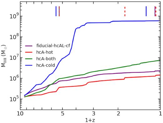
Evolution of the BH mass growth for the most massive BH in each of the simulated galaxies. Segments at the top of the figure highlight the redshift at which the considered BH experienced a BH merger. Note that at z ∼ 4.2 the BHs in fiducial–hcAL–cf, hcA–hot, and hcA–both have a merger.
The evolution of the central BH in fiducial–hcAL–cf is rather moderate: it spans roughly an order of magnitude in mass from z ∼ 8.5 (redshift at which the BH is seeded) to z = 0: it proceeds mainly via gas accretion until z ∼ 2, when it reaches a mass which is comparable to the final one. The low-redshift (z ≲ 2) difference in the mass evolution of the BH between fiducial–hcAL–cf and models hcA–hot and hcA–both is due to the different model of gas accretion on to the BH. The reason for the difference between BHs which continue accreting gas and increase their mass (hcA–hot and hcA–both) and the BH which does not (fiducial–hcAL–cf) stems from the suppressed accretion of cold gas with high angular momentum, rather than from the adopted feedback model. In Section 5.6, we discuss how the BH evolution and final results are sensitive to the details of gas accretion.
The different evolution of the three BHs in the models hcA–hot, hcA–both, and hcA–cold (the BHs of all these galaxies accrete both hot and cold gas according to equation 20) is due to the effect of the AGN when different models for coupling feedback energy to the multiphase ISM are adopted. In order to understand how feedback energy coupling affects the BH accretion and growth, we focus on the extreme cases represented by hcA–hot and hcA–cold. The reason for the intermediate behaviour of hcA–both follows directly.
When the AGN feedback energy is entirely coupled to the hot phase of the ISM, it increases its temperature (see Section 3.4). This causes an increase of pressure, that pushes the heated particle through nearly adiabatic expansion, thus triggering an outflow. Multiphase particles are hence displaced from the innermost regions of the galaxy: as a consequence, the density of the central regions feeding the BH decreases and the BH accretion rate is moderate. On the other hand, when all the feedback energy supplied to the multiphase ISM is provided to the cold component of multiphase particles, it is used to evaporate cold gas and to move its mass to the hot phase. However, this AGN-induced mass transfer does not produce a significant increase of the SPH temperature of the multiphase particle (see Appendix A). As a consequence, the multiphase gas remains close to the BH and enhances its accretion. Therefore, the BH experiences a rapid phase of mass growth, that will be halted when all the gas available within its surroundings is consumed. The BH mass growth is stopped (see Fig. 4, below z ≲ 2) and the central region of the galaxy appears devoid of gas (see the gas density map of hcA–cold in Fig. 2, where the central density depression has a radius which is comparable to the smoothing length of the BH at z = 0, see below). In this way, it is possible to explain why the evolution of the BH masses of hcA–hot and hcA–cold differ significantly from each other. In particular, from redshift z ≳ 4 on, the way in which the BH impacts on the overall evolution of the galaxy is remarkably different, especially because of the feedback energy budget involved.
We provide a more quantitative explanation by computing the mass of the gas that is located within 5 kpc from the galaxy centre and that is outflowing (i.e. with vr > 0, vr being the radial component of the particle velocity). The size of the region (a sphere with r = 5 kpc) that we choose to study the gas dynamics is roughly twice as large as the smoothing length of the BHs in hcA–hot and hcA–cold in the redshift range that we consider, i.e. 3 ≲ z ≲ 4. This redshift range identifies the time interval within which the difference between the evolution of the BH mass of hcA–hot and hcA–cold is magnified (even if the two evolutions are already different since z ∼ 8). Note that the BH smoothing length decreases below this redshift, reaching a size of ∼2.3 kpc at z = 0 for hcA–cold, while it is as small as 0.8 kpc at z = 0 for hcA–hot. The total mass of gas outflowing from the innermost regions at z = 4 and z = 3 for hcA–hot is detailed in Table 4, together with the corresponding shares of multiphase and single-phase outflowing gas.
Mass of gas outflowing from the innermost regions of hcA–hot, hcA–cold, and noAGN–reference.
| Simulation | z | |$M_{\rm outf,tot}$| | |$M_{\rm outf,mp}$| | |$M_{\rm outf,sp}$| |
|---|---|---|---|---|
| (M⊙) | (M⊙) | (M⊙) | ||
| hcA–hot | z = 4 | 1.4 × 10⁹ | 1.2 × 10⁹ | 2.1 × 10⁸ |
| z = 3 | 1.5 × 10⁹ | 1.3 × 10⁹ | 1.6 × 10⁸ | |
| hcA–cold | z = 4 | 7.4 × 10⁸ | 6.2 × 10⁸ | 1.2 × 10⁸ |
| z = 3 | 6.2 × 10⁸ | 4.9 × 10⁸ | 1.3 × 10⁸ | |
| noAGN–reference | z = 4 | 8.2 × 10⁸ | 7.0 × 10⁸ | 1.2 × 10⁸ |
| z = 3 | 8.5 × 10⁸ | 7.3 × 10⁸ | 1.2 × 10⁸ |
Note. Column 1: simulation label. Column 2: redshift. Column 3: total mass of gas outflowing from r ≤ 5 kpc. Column 4: mass of multiphase gas outflowing from r ≤ 5 kpc. Column 5: mass of single-phase gas outflowing from r ≤ 5 kpc.
Besides considering the simulation noAGN–reference, Table 4 also shows the same quantities for hcA–cold. These latter values are lower than those of hcA–hot by roughly a factor ∼2. This supports the interpretation that we provided.
Fig. 5 shows the position of the BHs of the four simulated galaxies on the plane of the Mbulge–MBH relation (Magorrian et al. 1998), that describes the correlation existing between the mass of the BH and that of the bulge of the host galaxy (see Section 1). For each simulated galaxy, we consider the mass of the BH, at z = 0, and the mass of the bulge of the galaxy. The mass of the bulge is estimated by performing a kinematic decomposition and considering only dispersion supported stars. We thus consider the gas particles within Rgal and assume that half of the bulge mass is made up of all the counter-rotating (Jz/Jcirc < 0) stars (see Section 5.3 and Fig. 8, for details). We compare results from simulations with observations from the sample by Kormendy & Ho (2013) and from the sample of McConnell & Ma (2013), which is made of 35 early-type galaxies (and whose best fit is provided by the red solid line). In their sample, Kormendy & Ho (2013) distinguish between elliptical galaxies, classical bulges in late-type galaxies and pseudo-bulges in late-type galaxies. Classical bulges are scaled-down versions of ellipticals, with which they share the formation scenario. On the other hand, pseudo-bulges are the outcome of the secular evolution they experienced within galaxy discs (Kormendy & Kennicutt 2004) and do not obey the same relation as the elliptical galaxies (Gadotti 2009; Kormendy & Bender 2012). This is evident from Fig. 5, where the majority of pseudo-bulges is located below the best fit to ellipticals only (red solid line), and are responsible for the bending of the Mbulge–MBH relation at Mbulge ≲ 5 × 10¹⁰ M⊙.
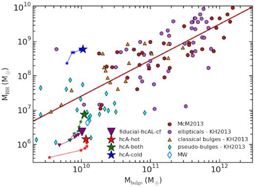
Mbulge–MBH relation for BHs in the simulated galaxies fiducial–hcAL–cf (purple triangle), hcA–hot (red starlet), hcA–both (green starlet), and hcA–cold (blue starlet). We also show the evolution tracks of the four models in the Mbulge–MBH plane from z = 3 down to z = 0. Symbols over each track pinpoint |$z = 3,2,1.5,1,0.5$|, and z = 0. Observations are from Kormendy & Ho (2013, KH 2013) and from McConnell & Ma (2013, McM 2013). The red solid line depicts the best fit to the 35 elliptical galaxies in the sample of McConnell & Ma (2013). The light-blue empty diamond shows the position of the BH in our Galaxy (Kormendy & Ho 2013).
Predictions from simulations are indicated by the purple triangle (fiducial model) and stars in Fig. 5: we also show the tracks of the four models from z = 3 down to z = 0, to outline their evolution on the Mbulge–MBH plane. Symbols over each track highlight the position of the systems at z = 3, z = 2, z = 1.5, z = 1, z = 0.5, and z = 0. The bulges of the galaxies that we have simulated have a formation history more similar to that of pseudo-bulges rather than to that of classical bulges: they indeed have grown within the galaxy as the galaxy itself grew more massive.4 Therefore, we consider as in agreement with observations those BHs that are located below the fit to the sample of elliptical galaxies only. The mass of the bulge for the considered galaxies at z = 0 is as follows: 1.02 × 10¹⁰ M⊙ for fiducial–hcAL–cf, 1.17 × 10¹⁰ M⊙ for hcA–hot, 1.10 × 10¹⁰ M⊙ for hcA–both, and 1.06 × 10¹⁰ M⊙ for hcA–cold. Fig. 5 shows that the BHs of the fiducial–hcAL–cf and hcA–both galaxies are in good agreement with observations. The BH of hcA–hot is quite in keeping with observations, as it lies on the lower edge of the region occupied by pseudo-bulges. On the other hand, the hcA–cold galaxy hosts a BH that is too massive for the bulge (and thus, the galaxy) in which it resides.
BHs are indeed expected to grow mainly at high-redshift (z ≳ 2), while at later times the AGN reaches a quasi self-regulated state, with AGN feedback roughly counterbalancing gas accretion and cooling. At approximately that point, the BH approaches the Mbulge–MBH relation, the BH accretion rate drops to lower values and gas accretion lies in the low-accretion mode regime. BHs of the simulated galaxies fiducial–hcAL–cf and hcA–both set on the Mbulge–MBH relation at 2 ≳ z ≳ 1. The way in which BHs climb the plane of the Mbulge–MBH relation proceeds along with the evolution of their mass shown in Fig. 4. Indeed, the mass of the bulge of these galaxies approaches by 2 ≳ z ≳ 1 a position close to that where they are at z = 0. Below this redshift range the bulge growth is not significant and mainly driven by processes that occur within the innermost region of the galaxy. For instance, considering the hcA–both galaxy, the mass of its bulge increases from 9.10 × 10⁹ M⊙ at z = 1.5, to 9.27 × 10⁹ M⊙ at z = 1, to 9.77 × 10⁹ M⊙ at z = 0.5, reaching then 1.10 × 10¹⁰ M⊙ at z = 0. Matching observations when the Mbulge–MBH relation is considered is a valuable benchmark for simulated galaxies, as this relation involves the BH mass and the stellar mass of the bulge of the host galaxy, that are quantities integrated throughout the galaxy evolution. In addition, the BH mass is also highly sensitive to details of the feedback process.
The location of BHs on the Mbulge–MBH plane is quite sensitive to the adopted feedback efficiency ϵf. This value is expected to have a crucial impact on final properties of BHs and to affect the normalization of the Mbulge–MBH relation: indeed, the higher the feedback efficiency is, the smaller the final mass of BHs is expected to be, as a larger amount of energy is provided to the ISM to counterbalance AGN feeding. We note that when the AGN feedback energy is entirely coupled to the cold phase of the ISM (hcA–cold) the BH has a final mass which grows beyond observations. We expect that a larger value of ϵf can compensate for the low response of the ISM to AGN feedback in this model.
In Appendix B, we will show how final results are sensitive to BH seed mass, and how we took advantage of the Mbulge–MBH relation to choose the reference |$M_{\rm BH,seed}$|.
5.3 BH-galaxy coevolution
In this section, we introduce the most important properties of the simulated galaxies presented in Section 5.1. Fig. 6 shows the star formation history of the five galaxies. With respect to the simulation noAGN–reference, the four galaxies including AGN feedback experience a comparable star formation history at early epochs (z ≳ 3), when the galaxy bulge forms. The comparison between some of the most pronounced star formation peaks highlights how the AGN usually has a positive feedback: for instance, the peaks at z ∼ 4 of fiducial–hcAL–cf and at z ∼ 2.3 of hcA–both are a clear evidence of this. Also, bursts in the evolution of the star formation can be related, relatively easily for hcA–both and hcA–cold, to peaks in the evolution of the BH accretion rate (see Fig. 3). None the less, a number of episodes where the AGN is found to have a negative feedback, suppressing star formation, are also present. The inclusion of the AGN clearly produces a positive feedback at low redshift (z ≲ 0.5), where the SFR is higher for simulations with AGNs. The reason for the enhanced star formation stems from the fact that AGN feedback energy overpressurizes the gas (see equations 10 and 11).

Star formation history for galaxies simulated with and without AGN feedback, colour-coded as explained in the legend.
AGN-induced overpressurization of gas can be quantified by comparing the pressure of multiphase gas particles that received feedback energy. Fig. 7 considers the simulation hcA–both and shows the pressure of all the multiphase gas particles which have been provided with AGN feedback energy, as a function of redshift. Particles’ pressure is evaluated at the beginning and at the end of each SPH time-step during which particles received feedback energy. The top panel of Fig. 7 considers the multiphase particles for which all the feedback energy supplied to the cold gas is used for the evaporation of the cold gas mass. The bottom panel describes the evolution of gas particles for which a fraction of the energy initially allocated to the cold phase is provided to the hot phase (see equation 37 and Section 3.4), as an additional contribution that ensures that no feedback energy is lost. In the bottom panel of Fig. 7 are thus considered those multiphase particles for which the cold phase is entirely evaporated by a single AGN feedback energy injection event. Solid curves depict the median evolution. The trend is the same for the two sub-samples of particles: nevertheless, in this way it is possible to appreciate the impact of the condition that guarantees that all the feedback energy is actually used (even if the multiphase gas particle that is provided with it has not enough mass of cold gas) and the number of particles that this condition involves (∼1/10 of the total number of multiphase particles selected for receiving feedback energy over the whole simulation). For the sake of concision, we show how the pressure of gas particles increases due to AGN feedback for the simulation hcA–both only. Similar conclusions can be drawn when considering all the other simulations, with the AGN-induced overpressurization of gas particles always becoming less significant as the redshift decreases. Pressure increase is mainly driven by direct heating of the multiphase ISM (see equations 31 and 36).
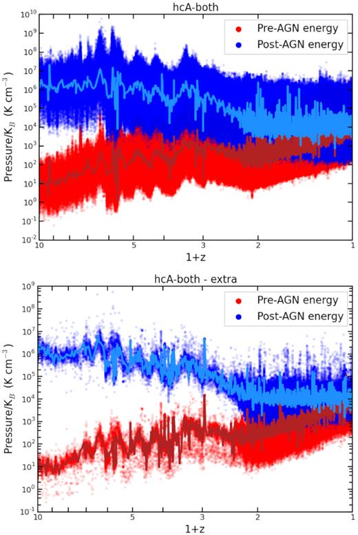
Pressure of multiphase gas particles before and soon after the feedback energy injection, as a function of redshift, for the simulation hcA–both. Solid curves show the median evolution. Top panel: evolution of gas particles for which all the feedback energy supplied to the cold gas is used for the evaporation of the cold gas mass. Bottom panel: evolution of gas particles for which a fraction of the energy initially allocated to the cold phase is provided to the hot phase, as an additional contribution that ensures that no feedback energy is lost.
The overpressurization of gas shown in Fig. 7 does not result in an enhanced SFR at all the redshifts (see Fig. 6: the star formation history of galaxies with and without the AGN feedback is comparable in the redshift range 2 ≳ z ≳ 0.5). This is due to the complex effect of AGN feedback, that also produces a concurrent overall heating of the forming galaxy and promotes massive outflows, thus reducing the gas reservoir available for star formation. These findings show that in our BH feedback scheme the negative effect is also important, so BH accretion is (partly) self-regulated. Moreover, numerical simulations have shown that the surrounding large-scale environment can provide high angular momentum gas through cold flows (Brooks et al. 2009; Pichon et al. 2011), and that the star formation feeding through cold flows decreases with cosmic time (Dubois et al. 2014b; Codis, Pichon & Pogosyan 2015). Within this picture, star formation in galaxies is mainly fuelled by cold gas accreted from outside the system itself at high redshift, this cold gas being able to reach the innermost regions of the forming galaxies where star formation occurs. This can explain why our galaxies with and without AGN feedback share a similar high-z star formation history, while the overpressurization of gas induced by the AGN since high-z turns out to be important at low-z. At low redshift the star formation is indeed mainly sustained by gas within the galaxy and by gas which falls back after its previous expulsion driven by stellar feedback, while the channel of external fuel through cold flows is by far subdominant.
The low-redshift enhanced star formation in galaxies simulated with AGN feedback with respect to the noAGN–reference simulation is responsible for more extended galaxy stellar discs (see also Fig. 2). Fig. 8 shows the distribution of stellar mass as a function of the circularity of the orbits of star particles, at z = 0, for the different simulations. The circularity of a stellar orbit is quantified by means of the ratio of specific angular momenta Jz/Jcirc, where Jz is the specific angular momentum in the direction perpendicular to the disc, and Jcirc is that of a reference circular orbit at a given distance from the galaxy centre (Scannapieco et al. 2009). Stars in the disc and in the bulge mainly contribute to the peak where Jz/Jcirc = 1 and Jz/Jcirc ∼ 0, respectively. The stellar disc component is remarkably larger in the simulations including AGN feedback with respect to the noAGN–reference galaxy. The evolution of the total stellar mass of the five galaxies is shown in Fig. 9. We analyse the total stellar mass within the galactic radius Rgal of the simulated galaxies (solid curves), and the contribution to the total from the stars in the bulge (dashed lines). We rely on the kinematic decomposition of the galaxy stellar component to assess whether a star particle belongs to the galaxy bulge (assuming that all the counter-rotating Jz/Jcirc < 0 stars make up half of the bulge mass, see also Figs 5 and 8). The drop in the evolution of the stellar mass of the bulge at z = 5.6 in Fig. 9 is due to an interacting substructure, which perturbs the morphology of the main galaxy progenitor and later merges with it. Bulge-over-total (B/T) mass ratios are lower (or equal, at most) for galaxies simulated with the AGN feedback; their z = 0 values,5 along with total and bulge stellar masses within Rgal are detailed in Table 5.

Circularity of star particles’ orbits for galaxies simulated with and without AGN feedback.

Evolution of the total stellar mass for galaxies simulated with and without AGN feedback. Solid lines show the total stellar mass within the galactic radius of each simulated galaxy, dashed curve highlights the contribution from the stellar mass in the bulge (as estimated from kinematic decomposition, see text and Fig. 8).
| Simulation | B/T | |$M_{\rm \ast ,tot}$| | |$M_{\rm \ast ,bulge}$| | Rgal |
|---|---|---|---|---|
| (M⊙) | (M⊙) | (kpc) | ||
| noAGN–reference | 0.41 | 2.68 × 10¹⁰ | 1.11 × 10¹⁰ | 24.03 |
| fiducial–hcAL–cf | 0.33 | 3.10 × 10¹⁰ | 1.02 × 10¹⁰ | 24.15 |
| hcA–hot | 0.41 | 2.83 × 10¹⁰ | 1.17 × 10¹⁰ | 24.18 |
| hcA–both | 0.38 | 2.87 × 10¹⁰ | 1.10 × 10¹⁰ | 24.15 |
| hcA–cold | 0.34 | 3.14 × 10¹⁰ | 1.06 × 10¹⁰ | 24.16 |
Note. Column 1: simulation label. Column 2: bulge-over-total mass ratio. Column 3: total stellar mass within Rgal. Column 4: stellar mass of the galaxy bulge. Column 5: galactic radius Rgal.
| Simulation | B/T | |$M_{\rm \ast ,tot}$| | |$M_{\rm \ast ,bulge}$| | Rgal |
|---|---|---|---|---|
| (M⊙) | (M⊙) | (kpc) | ||
| noAGN–reference | 0.41 | 2.68 × 10¹⁰ | 1.11 × 10¹⁰ | 24.03 |
| fiducial–hcAL–cf | 0.33 | 3.10 × 10¹⁰ | 1.02 × 10¹⁰ | 24.15 |
| hcA–hot | 0.41 | 2.83 × 10¹⁰ | 1.17 × 10¹⁰ | 24.18 |
| hcA–both | 0.38 | 2.87 × 10¹⁰ | 1.10 × 10¹⁰ | 24.15 |
| hcA–cold | 0.34 | 3.14 × 10¹⁰ | 1.06 × 10¹⁰ | 24.16 |
Note. Column 1: simulation label. Column 2: bulge-over-total mass ratio. Column 3: total stellar mass within Rgal. Column 4: stellar mass of the galaxy bulge. Column 5: galactic radius Rgal.
Fig. 10 shows the mass accretion history of the five galaxies, i.e. the evolution of the mass of gas that is accreted within their galactic radius. Galaxies share comparable accretion histories, except for some episodes where differences are evident. These discrepancies are the result of the internal gas dynamics: powerful outflows fostered by the joint activity of stellar and AGN feedback can reduce or even suppress for a while the accretion of gas from the large scale environment towards the innermost regions of galaxies (see Section 5.4).

Gas mass accretion history for galaxies simulated with and without AGN feedback. Evolution of the gas accreted within the galactic radius, i.e. |$R_{\rm gal} = 0.1 \, R_{\rm vir}$|.
Finally, Fig. 11 shows the radial profiles of gas and stellar surface density for the set of simulated galaxies, and provides complementary evidence to the gas and stellar density maps discussed in Section 5.1 (see Fig. 2). The most striking features are the drop in the gas density profiles of hcA–cold for r ≲ 2.5 kpc, and the external bump (25 kpc ≳ r ≳ 18 kpc) in the gas density profile of hcA–hot. The latter property is the outcome of recent gas accretion (Valentini et al. 2017).

Gas (solid curves) and stellar (dashed lines) surface density profiles for galaxies simulated with and without AGN feedback.
In summary, we find that the inclusion of the AGN mainly results in a positive feedback in our simulated spiral galaxies. Although we have shown that the SMBH negative effect is also important, AGN feedback is primarily positive: it pressurizes the multiphase gas, enhances the low-redshift star formation, and promotes the formation of more extended stellar discs. This result can be partly ascribed to our pressure-regulated star formation law. However, it goes beyond the numerical prescription adopted to estimate the molecular gas available for star formation, as there is accumulating (theoretical and observational) evidence that supports AGN-triggered star formation (e.g. Silk 2013; Bieri et al. 2015; Wagner et al. 2016; Cresci & Maiolino 2018). This conclusion is expected not to hold in simulations of elliptical galaxies, galaxy groups and clusters, as the AGN feedback is expected and observed to be mainly negative in these systems.
5.4 Galactic outflows
Galactic outflows in our simulated galaxies are the result of the joint activity of stellar and AGN feedback. They have a key role in regulating the cosmological accretion of gas from the large scale and in shaping both the expulsion of gas from the galaxy and the circulation of gas within and around the galaxy (see also Valentini et al. 2017). As an example, strong outflows at z = 2 in the hcA–cold simulation are responsible for the dip in the mass accretion history of this galaxy (Fig. 10), since they hinder gas accretion (note that we are now considering a different redshift range with respect to that analysed in Section 5.2). Outflow geometry in the aforementioned case is shown in Fig. 12: from the forming galaxy, at z = 2, a powerful bipolar outflow is launched, as shown by the light blue arrows pinpointing single-phase gas that is outflowing with a radial velocity that exceeds the escape velocity of the halo (i.e. vr > 268.5 km s−1). The lower panel of the same figure illustrates the corresponding case for the reference simulation without AGNs. The most striking feature that emerges from the comparison of the two panels in Fig. 12 is that the inclusion of AGN feedback promotes the formation of a (large-scale) bipolar outflow, while the geometry of the outflow in the noAGN–reference model is more isotropic. This result is independent of the details adopted in the AGN feeding and feedback modelling.

Geometry of the outflowing gas in the hcA–cold model and in the reference simulation with no AGNs, at z = 2. Single-phase gas is shown by red points, multiphase gas by green dots, and is mostly embedded within the innermost regions of the forming galaxy. Light blue arrows pinpoint gas that is outflowing with a radial velocity larger than the escape velocity of the halo (see Table 6 for details).
Galactic outflows involve both single-phase and multiphase gas. We estimate the mass of gas that is outflowing (i.e. which has a positive radial velocity vr) to quantify the impact of stellar and AGN feedback in driving outflows. We distinguish between single-phase and multiphase outflowing gas. The total gas mass involved in the outflows is given by the sum of the former ones. Table 6 provides outflowing gas masses for the simulations considered so far. The content of Table 6 is displayed in Fig. D1. We focus at redshift z = 2 and at z = 0. Besides considering gas which simply has vr > 0, we also estimate the mass of gas which is fostered to outflow with radial velocity exceeding 50 km s−1 (a reference threshold to get rid of gas whose motion could not emerge from the bulk motion within the galaxy, in observations) and the escape velocity of the halo at the considered redshift (vesc, detailed in Table 6). The contribution to the outflowing gas mass from the single-phase gas is larger by (at least) an order of magnitude than that coming from the multiphase gas. It is possible to quantify the impact of AGN-triggered outflows by contrasting the amount of gas which is outflowing in models with and without AGN feedback.
Mass of single-phase and multiphase gas involved in galactic outflows, for simulations fiducial–hcAL–cf, hcA–hot, hcA–both, hcA–cold, and noAGN–reference.
| Simulation | z | |$M_{\rm outf,mp}$| | |$M_{\rm outf,sp}$| | |$M_{\rm outf,mp}$| | |$M_{\rm outf,sp}$| | |$M_{\rm outf,mp}$| | |$M_{\rm outf,sp}$| | vesc |
|---|---|---|---|---|---|---|---|---|
| (M⊙) | (M⊙) | (M⊙) | (M⊙) | (M⊙) | (M⊙) | (km s−1) | ||
| vr > 0 | vr > 50 km s−1 | vr > vesc | ||||||
| fiducial–hcAL–cf | z = 2 | 1.94 × 10⁹ | 2.03 × 10¹⁰ | 7.41 × 10⁸ | 1.52 × 10¹⁰ | 1.49 × 10⁷ | 1.98 × 10⁹ | 268.3 |
| hcA–hot | z = 2 | 3.27 × 10⁹ | 1.81 × 10¹⁰ | 1.28 × 10⁹ | 1.26 × 10¹⁰ | 8.15 × 10⁶ | 1.74 × 10⁹ | 269.7 |
| hcA–both | z = 2 | 1.92 × 10⁹ | 1.91 × 10¹⁰ | 7.72 × 10⁸ | 1.36 × 10¹⁰ | 4.49 × 10⁵ | 4.67 × 10⁸ | 269.2 |
| hcA–cold | z = 2 | 1.50 × 10⁹ | 1.83 × 10¹⁰ | 7.65 × 10⁸ | 1.29 × 10¹⁰ | 1.39 × 10⁷ | 1.07 × 10⁹ | 268.5 |
| noAGN–reference | z = 2 | 2.20 × 10⁹ | 1.81 × 10¹⁰ | 7.33 × 10⁸ | 1.26 × 10¹⁰ | 5.66 × 10⁵ | 1.08 × 10⁹ | 270.2 |
| fiducial–hcAL–cf | z = 0 | 5.97 × 10⁹ | 5.46 × 10¹⁰ | 4.45 × 10⁸ | 5.14 × 10⁹ | 1.73 × 10⁶ | 1.92 × 10⁸ | 250.6 |
| hcA–hot | z = 0 | 9.69 × 10⁹ | 6.03 × 10¹⁰ | 7.59 × 10⁸ | 7.89 × 10⁹ | 1.61 × 10⁶ | 9.17 × 10⁷ | 250.9 |
| hcA–both | z = 0 | 7.62 × 10⁹ | 5.27 × 10¹⁰ | 2.77 × 10⁸ | 3.83 × 10⁹ | 2.46 × 10⁶ | 1.32 × 10⁸ | 250.5 |
| hcA–cold | z = 0 | 7.16 × 10⁹ | 4.90 × 10¹⁰ | 6.43 × 10⁸ | 5.73 × 10⁹ | 1.07 × 10⁶ | 3.42 × 10⁸ | 250.7 |
| noAGN–reference | z = 0 | 7.28 × 10⁹ | 5.19 × 10¹⁰ | 5.34 × 10⁸ | 4.54 × 10⁹ | 2.18 × 10⁶ | 1.22 × 10⁸ | 249.3 |
Note. Column 1: simulation label. Column 2: redshift. Column 3: mass of multiphase gas outflowing with radial velocity vr > 0. Column 4: mass of single-phase gas outflowing with radial velocity vr > 0. Columns 5 and 6: same as Columns 3 and 4, but considering gas with radial velocity vr > 50 km s−1. Columns 7 and 8: same as Columns 3 and 4, but considering gas with radial velocity vr > vesc. Column 9: escape velocity of the halo. Total gas mass in outflow is given by the sum of single-phase and multiphase gas involved in galactic outflows.
By focussing on the mass accretion history of hcA–both and hcA–cold in Fig. 10, at z ∼ 1, we see that outflows powered within galaxies that are experiencing a coevolution with SMBHs of different masses and accretion rates (see Figs 4 and 3, top panel) have a different interaction with the large scale environment. Also, from Fig. 10 we note the relative role of stellar- and AGN-driven outflows in regulating the accretion of gas, thus controlling the reservoir for star formation.
On average, by analysing the mass of outflowing gas, the contribution of AGNs to drive outflows in our simulations ranges between 20 and |$50 {{\ \rm per\ cent}}$| at z = 2 (see Table 6). The impact of AGNs is even more sub-dominant with respect to star formation-driven outflows at z = 0. Nevertheless, the role of AGN appears to be quite important in accelerating to high velocities the multiphase gas. Fig. 13 shows the radial component of the velocity for both single-phase and multiphase gas particles, as a function of their distance from the galaxy centre, at z = 2 (top row) and at z = 0 (bottom row). For reference, in Fig. 13, we also show the radial velocity for single-phase and multiphase gas particles when the AGN is not included. A larger amount of gas is launched to higher velocities in the inner region of the galaxy (r ≲ 30 kpc), when the AGN feedback is considered. We do not find a significant difference in the temperature of galactic outflows according to whether the AGN feedback is included or not (the hot phase temperature of the bulk of outflowing gas spanning the range ∼106–107 K). We do not find a significant evolution of the outflow temperature between z = 2 and z = 0: the hot gas temperature of outflowing particles is higher by a factor of ∼2 at most at z = 2 in the innermost regions of the galaxy.

Radial component of the velocity for single-phase (red) and multiphase (green) gas particles as a function of their distance from the galaxy centre, at z = 2 (top row) and at z = 0 (bottom row). From left to right: simulations hcA–both, hcA–cold, and noAGN–reference. The horizontal, dashed light blue line highlights the escape velocity of the halo for each model, while the dashed black line pinpoints the reference velocity threshold of vr = 50 km s−1.
To test the relative effect of SN- and AGN-triggered outflows in simulations, Costa et al. (2015), for instance, investigated the impact of AGN-driven outflows in cosmological simulations of high-redshift quasars. Interestingly, they found that the combined action of SN and AGN feedback produces the largest mass of both cold and hot gas to the highest outflow speed, with respect to the case in which the AGN feedback is not included. Biernacki & Teyssier (2018) found that AGN feedback is responsible for the formation of the hotter and lower density component of galactic outflows, and that it drives outflowing gas to larger distances from the galactic disc of simulated high-redshift galaxies. At variance with our findings, Koudmani et al. (2019) find that the AGN activity promotes outflows to temperatures and velocities which are higher by up to two orders of magnitude in dwarf galaxies, by using isolated galaxy simulations.
As highlighted by Veilleux, Cecil & Bland-Hawthorn (2005), it is hard to state whether a galactic wind is powered either by starburst and star formation activity only or by AGN activity alone. Recent observations have suggested correlations between outflow properties and ongoing AGNs and star formation activity in systems with different mass: these relations can be exploited to distinguish between different mechanisms of outflow triggering (Förster Schreiber et al. 2019). This topic represents a current challenge in cosmological simulations, too (e.g. Nelson et al. 2019). We found that both stellar and AGN feedback contribute to trigger outflows. The disc galaxies that we simulate including AGN feedback do not have an AGN-driven outflow component that makes galactic outflows differ significantly from those of galaxies simulated without including AGN feedback, as we have quantified by analysing outflow velocities and the mass of outflowing gas. The reason for this stems from the secondary role that AGN feedback is thought to play in systems of the same stellar mass as those that we are simulating. The picture emerging here is that AGN feedback in disc galaxies acts through a maintenance mode at low redshift, and provides a supporting role to stellar feedback.
5.5 Does AGN feedback affect metallicity profiles?
The goal of this section is to address the question of whether AGN feedback has an impact on the distribution of heavy elements within galaxies.
AGN-triggered galactic outflows can indeed promote the circulation of gas in and around galaxies, thus resulting in a modification of the heavy elements distribution. In addition, while launching outflows, SMBHs can modify the chemo-galactic ecosystem because they could either expel pristine gas at high redshift, that later falls back and dilutes the local metal content of the galaxy; or they could eject outwards gas enriched from stellar feedback, depriving of metals the innermost regions of galaxies. In order to assess the possible importance of these processes, the slopes and the normalizations of metallicity gradients can reveal vital information.
Fig. 14 shows the oxygen abundance radial profiles of gas in the simulated galaxies, at z = 0. Predictions from simulations are compared with observations from the sample of 130 nearby late-type galaxies of Pilyugin et al. (2014). The present-day Sun’s abundance in oxygen is taken from Asplund et al. (2009). Profiles of all the simulated galaxies are in agreement with observations. The simulations noAGN–reference and those including AGN feedback have almost indistinguishable metallicity profiles, that only show a slight difference beyond r ≳ 6 kpc from the galaxy centre (the discrepancy being as high as 0.1 dex at r = 10 kpc). The marginal difference at r ≳ 8 kpc between the noAGN–reference model and the other simulated galaxies is due to the AGN-stimulated star formation at z ≲ 0.1 (see Fig. 6), that results in recent star formation occurring in the outer regions of the galaxy disc. The stellar mass surface density of both fiducial–hcAL–cf and hcA–both at r = 10 kpc is twice as high as that of noAGN–reference (see Fig. 11).

Oxygen abundance gradients of gas in the simulated galaxies. Light blue profiles are observations from the sample of disc galaxies of Pilyugin, Grebel & Kniazev (2014), with shaded envelopes depicting the scatter of oxygen abundance around the trend.
The profiles of simulated galaxies share comparable slopes and normalization, this indicating that the AGN feedback does not affect significantly the distribution of heavy elements in the galaxy, at z = 0. The negligible effect of AGN feedback in shaping the metallicity gradients stems from the inability of AGN feedback to significantly affect the circulation of metals at large distance from the galaxy centre [the outermost radius considered in Fig. 14 is set by observational constraints, see Pilyugin et al. (2014)].
The picture emerging is that the normalization of the metallicity profiles is driven by the IMF (Valentini et al. 2019), while the AGN feedback has a negligible effect on them. The conclusions drawn in Valentini et al. (2019) as for the indication to prefer a Kroupa et al. (1993) IMF [more top-light with respect to the Chabrier-like Kroupa (2001)] for disc galaxies in the local Universe is confirmed and further corroborated when AGN feedback is included in our simulations.
To further investigate the possible role of AGN feedback in affecting the distribution of metals also at larger distances from the galaxy centre with respect to those considered in Fig. 14, we analyse gas metallicity maps. Fig. 15 shows the face-on and edge-on distribution of all the gas particles located within the galactic radius Rgal (see Table 5) of the fiducial–hcAL–cf and noAGN–reference galaxy simulations. We analyse the metallicity maps at redshift z = 0 and z = 2. The colour encodes the mean metallicity [Z/H] of the gas particles in each spatial bin. As for the present-day Sun’s metallicity, we adopt [Z/H]⊙ = 0.0207 ± 0.0015 (Bressan et al. 2012). The two galaxies simulated with and without AGN feedback share a comparable metal content at z = 0, the mean gas metallicity of the galaxy disc ranging from slightly supersolar to sub-solar (−0.4 ≲ [Z/H] ≲ 0.5). At z = 2, the galaxy fiducial–hcAL–cf which includes AGN feedback is characterized by lower metallicity gas in the innermost regions of the forming galaxy with respect to the case noAGN–reference, as we can appreciate by comparing panels in the third and fourth columns of Fig. 15. Galactic outflows drive a larger amount of both single-phase and multiphase gas in the galaxy fiducial–hcAL–cf with respect to the noAGN–reference model at z = 2 (see Table 6): in this way, they expel gas previously enriched in heavy elements. As the metallicity profiles shown in Fig. 14 highlight no significant differences at z = 0 between galaxies simulated with and without AGN feedback, we can conclude that the role of AGN-driven outflows in driving enriched gas out of the sites of star formation is episodic and mainly confined at higher redshift.
![Face-on (first and third columns) and edge-on (second and fourth) binned distributions of all the gas particles located within the galactic radius for the galaxy simulations fiducial–hcAL-cf and noAGN–reference. The colour encodes the mean [Z/H] of the gas particles in the bin. The distributions are shown at z = 0 (first and second columns) and at z = 2 (third and fourth ones).](https://oup.silverchair-cdn.com/oup/backfile/Content_public/Journal/mnras/491/2/10.1093_mnras_stz3131/1/m_stz3131fig15.jpeg?Expires=1750401857&Signature=wGVA~q-RCUoJq3jsBybjDsmQNn4Hfp8WKjWz5gquztW7J7oEY7uNzMT4Ydx1bcJ82hLD4RA7PzEIHwKe9u8l2VdcmZXsAsjJA63wKVjJj-znzWMiL3saHTRlPWHpVVLggskbyZyeqPg4T1hx9urfaq4nEPtmwtwiDs-sG~EyVIH~8aAEJbONOnMJsyfZpFYfhFYA15YViwzPpRj94ScAyhPNs~rtKzm9KOHk12onqdF8doYO5twnIJ5vc7~H5KrMouu6D1fSsVIKLlQXHpIjAlM6ArlsPfn9NggQ0gYZgSR3XCsegPkonEHUNgxhLFswcNN56Km72mv4vWVA86nYIg__&Key-Pair-Id=APKAIE5G5CRDK6RD3PGA)
Face-on (first and third columns) and edge-on (second and fourth) binned distributions of all the gas particles located within the galactic radius for the galaxy simulations fiducial–hcAL-cf and noAGN–reference. The colour encodes the mean [Z/H] of the gas particles in the bin. The distributions are shown at z = 0 (first and second columns) and at z = 2 (third and fourth ones).
5.6 Angular momentum dependent accretion
In this section, we investigate how different models of gas accretion on to the SMBH impact on final results. In particular, we study the effect that limiting accretion of the cold gas that is supported by rotational velocity has on the evolution of the central BH and on its mass at z = 0.
Fig. 16 shows the evolution of the BH mass as a function of the redshift. As in Section 5.2, we consider the most massive BH within a distance of 100 kpc from the galaxy centre. Vertical segments at the top of the figure record the redshift at which a BH merger occurred.

Evolution of the BH mass growth for the most massive BH in each of the simulated galaxies. Segments at the top of the figure highlight the redshift at which the considered BH experienced a BH merger, as in Fig. 4. Solid curves refer to simulations in which the SMBH accretes both hot and cold gas (hcA), while dashed curves identify the case of cold gas accretion only (ocA). All the simulations in this figure share the same AGN feedback model (both). See text for details on the labels.
All the simulations considered in Fig. 16 share the same AGN feedback model, with the AGN feedback energy which is provided to the multiphase medium being evenly distributed to the hot and cold phase. As for the AGN feeding, we consider four different models for BH gas accretion: (i) Bondi accretion of both hot and cold gas (hcA–both), (ii) Bondi accretion of cold gas only (ocA–both), (iii) modified Bondi accretion of hot and cold gas, where the accretion of cold gas with high angular velocity is limited according to equation (21) (hcAL2–both and hcAL3–both), (iv) modified Bondi accretion of cold gas only, which is limited according to its rotational support (ocAL–both). In the latter simulation, all the gas that contributes to accretion is controlled by the limiter |$\mathcal {L}_{\rm AM}$|. On the other hand, should the BH accrete both hot and cold gas, the limiter only controls cold gas accretion. The simulations hcAL2–both and hcAL3–both only differ from each other for the value of the parameter Cvisc that describes the viscosity of the cold gas supported by rotational velocity, at the sub-resolution level. The values of Cvisc that we explore are the following: |$C_{\rm visc} / 2 \, \pi = 1$| (ocAL–both) |$C_{\rm visc} / 2 \, \pi = 10^2$| (hcAL2–both), and |$C_{\rm visc} / 2 \, \pi = 10^3$| (hcAL3–both), and correspond to those considered by Schaye et al. (2015) and Crain et al. (2015).
As discussed in Rosas-Guevara et al. (2015), the parameter Cvisc encodes the sub-resolution parametrization of the viscosity. The factor |$\, \mathcal {L}_{\rm AM} = C_{\rm visc} ^{-1} \, (c_{\rm s,c} / V_{\phi })^3 \,$| (see equation 22), which reduces the Bondi accretion rate (see equation 21), is equivalent to the ratio between the Bondi time-scale and the viscous time-scale (tvisc, see below). Indeed, the presence of gas with a given amount of angular momentum introduces a characteristic spatial scale when modelling BH accretion, that is the size of the disc on which gas orbits before infalling on to the BH. Depending on the angular momentum of the gas, a typical timescale is set. This viscous time-scale enters the problem in addition to the Bondi time-scale, that is valid for gas accretion under the assumption that accreting gas does not rotate while infalling. The Bondi timescale reads: |$\, t_{\rm B} = r_{\rm B} / c_{\rm s} \,$|, where rB is the Bondi radius, i.e. the scale where the BH dominates over hydrodynamical processes (see Section 1), and cs is the sound speed of gas. The viscous timescale is proportional to the dynamical time, and can be cast as: |$\, t_{\rm visc} = [ \alpha _{\rm visc} \, (H/R)^2 ]^{-1} \, t_{\rm dyn} \,$| (see Rosas-Guevara et al. 2015, for further details). Here, R and H are the radius and the scale height of the accretion disc, respectively, while αvisc is a dimensionless parameter that is related to the kinematic viscosity. If the transport processes through the viscous accreting disc were fully understood, adequately accurate values for R, H, and αvisc would be inserted to model the effective accretion process. However, since we lack a full understanding of viscosity and accretion, and also considering that the accretion disc is far from being resolved in cosmological simulations, the ignorance is parametrized by means of |$\, C_{\rm visc} = 2 \, \pi \, [ \alpha _{\rm visc} \, (H/R)^2 ]^{-1} \,$|. In this way, a parameter is introduced in order to numerically capture the viscosity of gas in rotational support on a notional accretion disc, at the sub-resolution level. The (highly uncertain) value of the effective viscosity parameter Cvisc has been first explored by Rosas-Guevara et al. (2015), who proposed for it the range 103÷108. They adopted Cvisc = 2 × 10⁶ as fiducial value, and found that the larger is the value of Cvisc, the smaller is the mass of the hosted SMBH, for DM haloes as massive as ∼1012 M⊙. Note that Cvisc → ∞ would correspond to the case in which (cold) gas accretion on to the SMBH is not included. Also, note that large variations in Cvisc are required in order to have remarkable differences in the final results, since the suppression of the gas accretion by angular momentum needs |$\, C_{\rm visc} ^ {1/3} \, V_{\phi } \gt c_{\rm s} \,$| to result effective (see equation 22). Decreasing Cvisc corresponds to the situation in which the viscosity of the disc is higher and the gas accretion proceeds faster: indeed, viscosity transports angular momentum outwards, enabling accreting gas to spiral in towards the BH.
As a final remark, we note that state-of-the art cosmological simulations are still far from resolving the BH accretion disc (∼pc and sub-pc scale) and fully capturing the physics of processes which occur in the proximity of the BH. Quantities that enter |$\mathcal {L}_{\rm AM}$| (see equation 22) are estimated by considering the gas particles within the smoothing length of the BH (∼kpc scale, see Section 5.2). As a consequence, the value of Cvisc does not only parametrize the loosely constrained properties of BH accretion discs: it also encodes our ignorance of the unresolved processes occurring below the resolution limit of the simulation.
The evolution of the BH mass of hcA–both has been already considered in Fig. 4. Should only cold gas be accreted (ocA–both), the BH grows faster below z ≲ 1. Despite the accretion of a reduced amount of gas (with respect to hcA–both; note that the BH of ocA–both does not accrete the hot gas that is located within its smoothing sphere), the BH of ocA–both grows more massive and faster because of the reduced feedback. The gas in the proximity of the BH is denser in hcA–both than in ocA–both (by a factor of ∼2 at z = 1, and by a factor of ∼1.5 at z = 0, at r = 1 kpc from the galaxy centre).
When the limiter to the accretion of cold gas that is supported by rotational velocity is accounted for, the evolution of the BH mass changes: reducing the accretion of cold gas delays or even suppresses the BH growth. The higher the values of Cvisc that are adopted, the more significant is the BH growth reduction. Focussing on hcAL2–both, the BH mass growth is hindered below z ∼ 4; finally, the BH is prevented from growing below z ∼ 2, aside from a BH merger at z ∼ 0.2. The BH growth by gas accretion is even stopped when |$C_{\rm visc} / 2 \, \pi = 10^3$| (hcAL3–both) is adopted. With respect to the reference simulation hcA–both, the BH mass at z = 0 is reduced by an order of magnitude or even more, the BH masses being 1.10 × 10⁶ M⊙ (hcAL2–both) and 4.48 × 10⁵ M⊙ (hcAL3–both).
The scenario that emerges from Fig. 16 has interesting implications for the formation and evolution of disc galaxies. Indeed, the fundamental connection between the MBH and Mbulge implies that the growth of the BH is tightly linked to the formation of galaxy bulges (Kormendy & Ho 2013). Even if the coevolution with pseudo-bulges is not as close as for classical bulges, BHs do not correlate with the properties of galaxy discs (Kormendy & Gebhardt 2001; Kormendy & Bender 2011; Kormendy & Ho 2013). As a consequence, the SMBH hosted in a late-type galaxy is expected to grow mainly at high-redshift, while the formation of the bulge of the galaxy proceeds. On the contrary, the BH growth is limited at low-redshift, when the formation of the galaxy disc occurs (e.g. Greene, Ho & Barth 2008; Shankar et al. 2012).
Fig. 16 shows that this is the case for hcAL2–both: below redshift z ∼ 3 ÷ 2 the growth of the BH through gas accretion is almost insignificant. Below redshift z ∼ 2, the BH mass only grows as a consequence of mergers with other BHs. The effect of the limiter |$\mathcal {L}_{\rm AM}$| is clearly evident when considering the simulated galaxy hcAL3–both: below redshift z ∼ 4, the growth of the BH by gas accretion is suppressed, and the BH mass evolution is driven by mergers alone. As the formation of the bulge and of the disc of our simulated galaxies typically occurs above and below z ∼ 3 ÷ 2, respectively (see Fig. 6 and Valentini et al. 2019), what emerges from Figs 16 and 17 is that once the angular momentum of the cold gas that is accreting on to the central BH is taken into account, the aforementioned scenario for BH-disc galaxy coevolution is successfully reproduced.

Same as Fig. 16, but considering other simulations which also include our fiducial model.
Fig. 17 shows the evolution of the BH mass as a function of the redshift for another suite of simulations, including our fiducial model. The simulation hcA–cf has an SMBH that grows in a way that is similar to that of hcA–both. The effect of suppressing the accretion of high angular momentum cold gas reduces the BH mass of hcAL2–cf (wrt hcA–cf) at z = 0 by an amount that is comparable to what obtained in hcAL2–both (wrt hcA–both). This figure illustrates that the conclusions drawn so far when discussing Fig. 16 are still valid when AGN feedback energy is distributed to the multiphase ISM according to the physical properties of the gas.
The scenario of BH merging as the most viable channel for BH growth in galaxies within haloes of ∼1012 M⊙ has been pointed out by Bonoli et al. (2016), who presented a detailed study of the coevolution of an MW-sized simulated galaxy and its SMBH. Interestingly, they found that the SMBH growth is mainly due to the mergers with other BHs located within satellites approaching the forming galaxy, rather than to gas accretion. At z = 0, their simulated galaxy hosts a BH as massive as 2 × 10⁶ M⊙.
The suppression of the low-redshift BH growth due to the angular momentum limiter is evident when the BH accretes both the hot and cold gas (solid curves in Fig. 16), as well as when the BH only accretes cold gas (dashed curves). Should only cold gas be accreted, a lower value of Cvisc is enough to have roughly the same BH mass reduction that is observed with a higher value of Cvisc when the BH accretes both the hot and cold gas. Indeed, the difference between the final BH mass of ocAL–both (3.61 × 10⁶ M⊙) and of ocA–both (3.46 × 10⁷ M⊙) is comparable to that which distinguishes hcAL2–both from hcA–both. Therefore, when only cold gas accretion is considered, the delay and suppression of the BH mass growth is obtained by assuming a higher viscosity for the disc on which the accreting gas is settled, i.e. by assuming an accretion not as impeded as if it involved both hot and cold gas.
The values of Cvisc for hcAL2–both and hcAL3–both are the ones adopted in the EAGLE simulations (Schaye et al. 2015). They adopt |$C_{\rm visc} / 2 \, \pi = 10^2$| for the simulation of their suite at lower resolution (in which the initial mass of gas particles is larger than that of AqC5 by a factor 4.4, see Section 4), and |$C_{\rm visc} / 2 \, \pi = 10^3$| for their higher resolution run (where the initial mass of gas particles is smaller than that of AqC5 by a factor 1.8). Indeed, Crain et al. (2015) explored the variation on galaxy scaling relations produced by different values of Cvisc (they considered the following values: |$C_{\rm visc}/ 2 \, \pi = 0.01,1,100$|), to quantify the impact of the sub-resolution viscosity in calibrating the EAGLE simulation. They found that their model for AGN feedback is primarily dependent on Cvisc. Also, they found that larger values of Cvisc delay the BH growth via gas accretion and the quenching of star formation by AGN feedback. Also, they observed that the higher is the value of Cvisc, the lower is the BH mass corresponding to a determined stellar mass (of the bulge) of the host galaxy. Our results are thus in keeping with Crain et al. (2015). As a future direction of investigation, it would be interesting to explore how the aforementioned scenario of low-redshift suppression of gas accretion fits within the framework of Seyfert galaxy evolution, being gas accretion the most viable channel for BH mass growth at low redshift in these systems.
5.7 Overview of previous works and comparison
In this section, we focus on the modelling of AGN feedback in a multiphase ISM and on the positive AGN feedback which enhances star formation. The physical idea behind our modelling is in line with results from several higher resolution (∼pc) simulations which explicitly model the clumpy, multiphase ISM (e.g. Gaibler et al. 2012; Wagner, Bicknell & Umemura 2012; Wagner, Umemura & Bicknell 2013). For instance, Wagner et al. (2013) resolve a two-phase ISM, where the cold clouds are in pressure equilibrium with the hot ambient medium. Once the cold gas receives AGN feedback energy, it is progressively eroded and disperses; the hot gas receives the bulk of the feedback energy, which is deposited mostly in thermal form, and is pushed to further distances. Interestingly, they find that when the cold clouds are distributed in a disc, the AGN feedback uplifts them from the galactic plane and compresses the gas, while the warm gas in the disc inflows towards the galaxy centre shortly after. The interaction between AGN-driven outflows and the multiphase ISM often results in a positive feedback, with jet-induced and pressure-triggered star formation (Gaibler et al. 2012; Wagner et al. 2012). Final results are not sensitive to the opening angle of the AGN jet (Wagner et al. 2013), while the cross-section of cold clouds (to be related to the covering factor in our modelling) determines how effective is the response of the cold ISM to the AGN feedback energy injection (Wagner et al. 2012). High-resolution simulations by Bourne, Nayakshin & Hobbs (2014) and Bourne, Zubovas & Nayakshin (2015) investigating the impact of outflows from an SMBH on the ISM of the innermost region of a galaxy show that the bulk of feedback energy is coupled to the hot phase and carried away from the centre of the host through paths of least resistance within the clumpy multiphase ISM; on the other hand, the bulk of the momentum is coupled to the cold component. Interestingly, Bourne et al. (2015) discuss how an adequately high-resolution and a detailed modelling of the ISM is crucial to recover the AGN-induced compression, this result being missed in lower resolution simulations and the negative effect of the AGN feedback being thus overpredicted.
High-resolution simulations with idealized and simplified initial conditions which study the impact of AGNs outflows on a multiphase ISM are also important to understand where the AGN-triggered star formation is expected to occur. For instance, Nayakshin & Zubovas (2012) find that star formation bursts are produced within thin and dense layers of cold gas surrounding the shocked and compressed hot gas out of which they form (see also Zubovas et al. 2013). Zubovas & Bourne (2017) discuss the twofold role of AGN-triggered outflows, which can either suppress or enhance star formation, in line with our results. They find that spots of AGN-induced star formation are located in cold and dense knots of gas which get compressed within hot feedback bubbles (see also Zubovas, Sabulis & Naujalis 2014); also, star formation occurs at the outer edge of the hot outflow bubble, highlighting that AGN outflows compress swept up gas and locally induce star formation. Clumps with ongoing star formation can also form along the backflow of AGN inflated bubbles, the backflow ultimately reaching the galaxy disc, where further star formation is triggered (Silk 2013; Bieri et al. 2016).
6 CONCLUSIONS
We introduced a novel model for AGN feedback and implemented it within the sub-resolution model MUPPI, already featuring cooling, star formation, stellar feedback, and chemical enrichment. We carried out a suite of cosmological hydrodynamical simulations of disc galaxies, with zoomed-in initial conditions leading to the formation of a halo of mass |$M_{\rm halo,DM} \simeq 2 \times 10^{12}$| M⊙ at redshift z = 0. These simulations have been designed to investigate
the effect of different ways of coupling AGN feedback energy to the hot and cold phases of the multiphase ISM;
the impact of different models of gas accretion on to SMBHs, namely only cold gas, both cold and hot gas, with the additional possibility of limiting gas accretion from cold gas with high angular momentum;
how different models of gas accretion and AGN feedback energy coupling affect the overall BH-galaxy coevolution.
We investigated the effect that coupling AGN feedback energy to the different phases of the ISM has on the evolution of SMBHs. Providing to the hot phase the entire budget of feedback energy, or a considerable fraction of it, produces an SMBH that grows in mass by up to one or two order of magnitudes from z ∼ 8.5 to z = 0. Its final mass ranges between ∼106 and ∼107 M⊙. On the other hand, when the AGN feedback energy is entirely supplied to the cold phase, the multiphase ISM is not promoted to outflow and remains close to the BH: as a consequence, the BH experiences a rapid phase of mass growth (in the redshift range 3 ≲ z ≲ 5) during which it deprives of gas the centre of the host galaxy, and then its growth is suppressed. The BH mass at z = 0 can be as high as ∼109 M⊙ in this case. Therefore, a prediction of our model is that at least a share of the AGN feedback energy has to couple with the diffuse hot gas.
We examined the effect of coupling the AGN feedback energy injected in a multiphase ISM to its phases according to their physical properties. We considered a model where feedback energy coupling is driven by the covering factors of the hot and cold phases, assuming that the larger is the volume occupied by the cold gas clumps, the larger is the amount of energy that the cold gas absorbs.
Gas accretion is the process that contributes the most to the BH growth, rather than mergers with other BHs (Section 5.2). Throughout BH evolution, the total accretion rate is dominated by cold gas accretion, with respect to hot. Remarkably, this is in line with Gaspari et al. (2019), even if they derived such a conclusion by means of a phenomenological analysis focused on more massive systems. Our conclusion that gas accretion is a more viable channel for BH growth than BH mergers is true unless cold gas which is supported by rotational velocity is prevented from accreting (see below). The quiet merging history that characterizes our simulated disc galaxies also contributes to the minor role of BH mergers to the BH mass growth. The contribution to the BH growth by BH–BH mergers is expected to become more significant for increasing BH mass (Fanidakis et al. 2011; Dubois, Volonteri & Silk 2014a; Weinberger et al. 2018).
We find that when the BH only accretes cold gas, it experiences a growth by gas accretion that is faster than (or at most comparable to) the case in which both cold and hot gas are accreted. As for the galaxy Mbulge–MBH scaling relation, predictions from simulations are in keeping with observations, considering a BH seed mass as large as ∼105 M⊙.
When the accretion of cold gas that is supported by rotational velocity is reduced, the BH mass growth is delayed and the BH mass at z = 0 is reduced by up to an order of magnitude with respect to the case in which both hot and cold gas accretion proceed unimpeded. Within the scenario emerging from this model, the SMBH in MW-sized galaxies is prevented from growing by gas accretion below z ≲ 2, aside from possible BH mergers. Also, the lower is the viscosity assumed for the cold gas which is accreting (i.e. the larger Cvisc), the more the BH mass growth is reduced.
Simulations that include AGN feedback produce spiral galaxies with a more extended stellar disc component. The SMBH mainly produces a positive feedback in our simulated late-type galaxies, pressurizing the multiphase gas and ultimately enhancing the low-redshift star formation. We expect that this conclusion changes when we will simulate elliptical galaxies, galaxy groups and clusters, where the AGN feedback is supposed to be mainly negative.
Including AGN feedback does not affect the slope nor the normalization of metallicity gradients at low redshift. As a consequence, we can conclude that the energy injection and especially the outflows driven by the SMBH (Section 5.4) do not alter significantly the circulation of metals within galaxies (Section 5.5).
AGN feedback operates in a wide class of systems, from galactic bulges to massive galaxy clusters. In this work, we studied the way in which AGN feedback energy is coupled to the different components of the ISM focussing on late-type galaxies: however, AGN feedback is expected to play a supporting role in MW-sized galaxies, where the central BH contributes to determine the properties of the bulge and shape the galaxy innermost regions. A forthcoming extension of this study is to include elliptical galaxies in the analysis, so as to investigate how the AGN affects the formation and evolution of systems characterized by more massive BHs accreting at higher rates. Also, we plan to investigate the effect of stellar and AGN feedback on the properties of simulated galaxy populations, instead of those of single galaxies.
At the same time, it would be interesting to further investigate hot gas haloes in massive spiral galaxies. Valentini & Brighenti (2015) studied the hot gas cooling process triggered by AGN feedback in models of low-mass ellipticals: provided the similarity between the hot ISM of these systems and detected hot coronae around disc galaxies, it appears likely that any outburst from the central BH could promote cooling of the hot corona, generating cold clouds that would accrete on the galactic disc.
As for the modelling of AGN feedback, a further direction for improvement is provided by the additional work that is required to numerically account for the mechanical component of AGN-triggered outflows. In the model that we have introduced, all the AGN feedback energy is coupled thermally and isotropically to the surrounding medium, with a constant efficiency. Besides the radiative feedback, our implementation is thus still missing the modelling of the mechanical AGN feedback, that is considered to be the dominant channel in which the AGN operates for low-activity stages (i.e. low accretion rates) of the BH (radio mode). Moreover, we have here followed a rather simplified approach also for the modelling of gas accretion on to SMBHs. Albeit the Bondi-like accretion is adopted in the majority of cosmological simulations nowadays, and despite having corrected it by taking into account the angular momentum of cold gas which is accreted, we aim at achieving a more accurate description of the BH accretion in the near future. A desirable possibility to attain is the so-called chaotic cold accretion (Gaspari et al. 2013; Gaspari, Temi & Brighenti 2017), where cold blobs condensed out of the hot ambient medium fall on to the SMBH and are accreted after they undergo chaotic inelastic collisions. In this way, the BH accretion rate is boosted and the AGN activity consists of frequent bursts. The modelling of this regime for AGN feeding will be a key one especially once processes such as cooling, heating, turbulence, and rotation are consistently accounted for and the resolution is increased. This will be extremely important when considering more massive systems.
Another quite interesting challenge would be to compare predictions from these simulations to observations at high redshift, in order to better constrain the BH growth across cosmic time and interpret possible scenarios of galaxy evolution.
ACKNOWLEDGEMENTS
We thank the anonymous referee for the careful and constructive report that helped improving the presentation of results. We thank Volker Springel for making the gadget3 code available to us. We are grateful to Lucio Mayer, Gabriella De Lucia, Klaus Dolag, Annalisa Pillepich, Massimo Gaspari, and Filippo Mannucci for constructive discussions and feedback. SB acknowledges financial support from PRIN-MIUR 2015W7KAWC, the agreement ASI-INAF n.2017-14-H.0, the INFN INDARK grant. SB, GM, GG, and LT are also supported by the EU H2020 Research and Innovation Programme under the ExaNeSt project (Grant Agreement No. 671553). AB and AL acknowledge support by PRIN MIUR 2017 prot.20173ML3WW 002 ‘Opening the ALMA window on the cosmic evolution of gas, stars and supermassive black holes’. Simulations were carried out using ULISSE at SISSA, Marconi at CINECA, and the Trieste ‘baastet’ cluster at INAF-Osservatorio Astronomico di Trieste (Italy). CPU time has been assigned through the project Sis18_bressan under Convenzione SISSA, through the project INA17_C1A00, and through Italian Super-Computing Resource Allocation (ISCRA) proposals and an agreement with the University of Trieste. The post-processing has been performed using the PICO HPC cluster at CINECA through our expression of interest.
Footnotes
This scheme for repositioning the merged BH leads to a violation of the momentum conservation law (see e.g. Hirschmann et al. 2014).
When the cold gas evaporates, we increase for simplicity its internal energy and neglect the |$P \, \mathrm{ d} V$| work contribution, assuming that hydrodynamical forces account for it in the following time-step. Equation (33) indeed provides a slight overestimation of |$\dot{M}^{\rm AGN}_{\rm c,th }$|. The energy rate |$\dot{E}^{\rm AGN}_{\rm c }$| should actually be divided by |$\,\frac{{{k}}_{\rm B} \, (T_{\rm h} - T_{\rm c})}{(\gamma -1) \, \mu _{\rm c} \, m_{\rm p}} + \frac{P_{\rm c}}{\rho _{\rm h}}\, \,$|, where Pc/ρh represents the |$P \, \mathrm{ d} V$| work done against the hot gas, and Pc = Ph due to the pressure equilibrium between the gas phases. Should this correction be taken into account, equation (33) becomes: |$\,\dot{M}^{\rm AGN}_{\rm c,th } = \dot{E}^{\rm AGN}_{\rm c } \, \frac{(\gamma -1) \, \mu _{\rm c} \, m_{\rm p}}{{{k}}_{\rm B} \, (\gamma \, T_{\rm h} - T_{\rm c})} \, \,$|. The factor 1.67 by which the hot gas temperature would be increased introduces a contribution which can be considered within the uncertainty of the parameters of the model.
We define here the galactic radius as one-tenth of the virial radius, i.e. Rgal = 0.1Rvir. The radius Rgal is chosen to select the region of the computational domain where the central galaxy resides. We consider virial quantities as those computed in a sphere that encloses an overdensity of 200 times the critical density at present time and that is centred on the minimum of the gravitational potential of the halo.
We postpone to a forthcoming work a proper classification and an extensive investigation of the formation path of the bulges of the galaxies that we have simulated.
Note that the B/T values that we quote should not be directly contrasted with observational photometric ones, as our estimates for the B/T ratio could also include satellites, stellar streams, and contribution from bars within Rgal. Halo stars are also included when estimating the dispersion supported component. Photometric determination for the value of B/T is lower than the corresponding kinematic estimate (Scannapieco et al. 2010).
REFERENCES
APPENDIX A: CONSTANT COUPLING PARAMETERS
We consider three different possibilities as test cases to investigate how AGN feedback energy couples to the surrounding multiphase ISM:
All the energy is provided to the hot gas phase (|$\mathcal {A}_{\rm h}=1$| and |$\mathcal {A}_{\rm c} = 0$|).
AGN feedback energy is entirely supplied to the cold component (|$\mathcal {A}_{\rm h}=0$| and |$\mathcal {A}_{\rm c} = 1$|).
The energy assigned to each multiphase particle is evenly shared among the hot and cold gas (|$\mathcal {A}_{\rm h}=0.5$| and |$\mathcal {A}_{\rm c} = 0.5$|).
As a consequence, assuming |$\mathcal {A}_{\rm h}=\mathcal {A}_{\rm c} = 0.5$|, the hot gas mass and thus the hot gas density can increase by up to a factor of ≲2, at most. Therefore, the hot gas phase will not experience a runaway cooling, and the SPH temperature of the multiphase particle is not expected to change significantly due to the AGN-induced transfer of cold gas to the hot phase.
APPENDIX B: EFFECT OF BH SEED MASS
The initial mass assumed for BHs in cosmological simulations (see Section 3.1) is rather important, and has fundamental implications for theoretical models, as it is linked to the mass of SMBH progenitors and to viable scenarios of SMBH formation. The value adopted for the BH seed mass is crucial when simulating MW-sized galaxies (i.e. |$M_{\rm halo,DM} \simeq 10^{12}$| M⊙ at redshift z = 0) in a cosmological context: indeed, since BH growth due to gas accretion is relatively moderate in these galaxies, final results are quite sensitive to the value adopted for |$M_{\rm BH,seed}$|.
The adopted value of |$M_{\rm BH,seed}$| is closely connected to the choice of MDM,thresh (see Section 3.1). Indeed, a lower mass threshold MDM,thresh for the DM halo within which BHs can be seeded translates directly to the introduction of the BH at higher redshift. In this section, we explore the impact that the value assumed for |$M_{\rm BH,seed}$| has on final results. We consider the following values for BH seed masses: |$M_{\rm BH,seed} = 1.1 \times 10^5$| M⊙ (reference value), |$M_{\rm BH,seed} = 5.5 \times 10^4$| M⊙ (S0.5x), and |$M_{\rm BH,seed} = 2.7 \times 10^5$| M⊙ (S2x) (see Table 3). BH seeds as massive as ∼105 M⊙ would correspond to a formation scenario for SMBHs by direct collapse (e.g. Begelman et al. 2006).
We consider a first set of three simulations: hcA–both, hcA–both–S0.5x, and hcA–both–S2x (see Table 3). They share the same set-up and physics, and they only differ for the assumed |$M_{\rm BH,seed}$|.
Masses of their BHs at z = 0 are as follows: MBH = 7.4 × 10⁶ M⊙ (hcA–both), MBH = 7.7 × 10⁵ M⊙ (hcA–both–S0.5x), and MBH = 1.2 × 10⁷ M⊙ (hcA–both–S2x). Fig. B1 shows the Mbulge–MBH relation for the simulated galaxies. We compare the outcome of the three simulations (identified by stars) to observations (see Section 5.2). The seed mass of the BHs is indeed commonly calibrated in order to reproduce observed scaling relations at redshift z = 0. The simulation adopting |$M_{\rm BH,seed} = 1.1 \times 10^5$| M⊙ is the one that best agrees with observations. A BH seed mass as large as twice the reference value also leads to a good agreement with observations. On the other hand, decreasing |$M_{\rm BH,seed}$| by a factor of ∼2 with respect to the fiducial value, would decrease the MBH at z = 0 by an order of magnitude. This worsens significantly the matching with observations in Fig. B1. It is not straightforward to relate the BH seed mass to other properties of the simulated galaxies, and to highlight definite trends. For instance, hcA–both, hcA–both–S0.5x, and hcA–both–S2x have the following stellar mass: 2.87 × 10¹⁰, 2.58 × 10¹⁰, and 2.07 × 10¹⁰ M⊙, respectively. As for their bulge-over-total mass ratios, the B/T of hcA–both, hcA–both–S0.5x, and hcA–both–S2x is as follows: 0.38, 0.37, and 0.60, respectively.

Mbulge–MBH relation for BHs in the simulated galaxies where different BH seed masses are considered (see Table 3). Simulations pinpointed by starlets assume both cold and hot gas accretion (hcA), while simulations identified by triangles assume only cold gas accretion (ocA). Observations are from Kormendy & Ho (2013, KH 2013) and from McConnell & Ma (2013, McM 2013), as in Fig. 5.
We also consider three additional simulations: ocA–both, ocA–both–S0.5x, and ocA–both–S2x. They are analogous to the first set as for the adopted BH mass seeds and model of the coupling of AGN feedback energy, but the BH in these simulations only accretes cold gas (see Table 3). In this way, we investigate whether the prediction for the most suitable value of |$M_{\rm BH,seed}$| is unchanged when the details of the gas accretion modelling are varied. At z = 0, the most massive BH within each of the simulated galaxy has the following mass: 3.5 × 10⁷ M⊙ (ocA–both), 1.3 × 10⁶ M⊙ (ocA–both–S0.5x), and 6.0 × 10⁷ M⊙ (ocA–both–S2x). The stellar mass of the bulge of simulated galaxies does not depend on whether only cold or both hot and cold gas is accreted.
For this second set of simulations (triangles), the lowest value for |$M_{\rm BH,seed}$| leads to a simulated galaxy on the edge of the region of the Mbulge–MBH relation where observations are found. The reference and the highest values for |$M_{\rm BH,seed}$| predict an SMBH that is located in the upper edge of the region of the plane occupied by pseudo-bulges. When only cold gas accretion is assumed, BHs grow more massive than the case in which both hot and cold gas accretion is considered.
The location at z = 0 of an SMBH on the plane of the Mbulge–MBH relation loosely constrains the way in which it coevolved with its host galaxy. However, when |$M_{\rm BH,seed}=1.1 \times 10^5$| M⊙ is adopted, the BH is required to roughly increase its mass by an order of magnitude or slightly more between the redshift z at which it has been seeded and z = 0. Such a requirement seems to favour the scenario according to which SMBHs accrete both hot and cold gas, at least when the reference seed mass is adopted and when the AGN feedback energy provided to the multiphase ISM is evenly shared by the hot and the cold phase. All the BHs in the simulations considered are seeded at z ∼ 8.5: this redshift is closely related to the (fixed) value of MDM,thresh.
As a consequence, we adopt |$M_{\rm BH,seed}=1.1 \times 10^5$| M⊙ as the fiducial value for the BH mass seed. Albeit the exploration of the parameter space for |$M_{\rm BH,seed}$| has been carried out for a single galaxy rather than for galaxies in a cosmological box, and even if resolution effects can enter the calibration, the reference value for |$M_{\rm BH,seed}$| can be considered as representative of typical progenitors of MW-sized BHs at z = 0. According to predictions from the simulations considered here, SMBH progenitors as massive as ∼105 M⊙ should already be in place at redshift z ≳ 8. This poses a challenging question from a theoretical perspective (Begelman et al. 2006), given the age of the Universe at that time (∼0.6 ÷ 0.7 Gyr).
APPENDIX C: Effect of ℓMC
In this section we investigate the impact of the parameter ℓMC, describing the typical size assumed for clumps within molecular clouds (see Section 3.6.1). It enters in the sharing of AGN feedback energy among the hot and the cold phase of the multiphase ISM: the lower ℓMC, the larger |$\mathcal {C}_{\rm c}$|, when a multiphase particle with given physical properties is considered (see equation 38).
We consider four simulations: hcA–cf, fiducial–hcAL–cf, hcA–cf–20pc, and hcAL–cf–20pc. They adopt either ℓMC = 1 pc or ℓMC = 20 pc (see Table 3). Further test runs carried out adopting ℓMC = 5 pc and ℓMC = 30 pc confirm the trends outlined here. For instance, the mean values for |$\mathcal {C}_{\rm h}$| and |$\mathcal {C}_{\rm c}$| in the simulation hcAL–cf–20pc are ∼0.76 and ∼0.24, respectively. The fiducial model fiducial–hcAL–cf has the following mean values for |$\mathcal {C}_{\rm h}$| and |$\mathcal {C}_{\rm c}$|: 0.41 and 0.59 (see Section 5.1).
Fig. C1 shows the position of the BHs of the simulated galaxies on the plane of the Mbulge–MBH relation. The comparison with observations highlights that hcA–cf–20pc and hcAL–cf–20pc lie on the lower edge of the region occupied by pseudo-bulges. This implies that a smaller value of ℓMC has to be preferred, that is also in better agreement with what observations suggest (e.g. Williams et al. 1994; Bergin & Tafalla 2007; Muñoz et al. 2007; Gómez et al. 2014, and references therein; see Section 3.6.1).

APPENDIX D: EVOLUTION OF OUTFLOWING GAS
In this section we show the evolution of the mass of multiphase and single-phase gas involved in outflows. Fig. D1 displays the content of Table 6 (see Section 5.4 for details).

Mass of multiphase (top panel) and single-phase (bottom panel) gas which is outflowing with positive radial velocity (circles) or radial velocity exceeding 50 km s−1 (squares) and the escape velocity of the halo (diamonds; see Table 6 for details). Quantities are analysed at redshift z = 2 (open symbols) and z = 0 (filled symbols).
