


ABSTRACT
Supernovae (SNe) could be powerful probes of the properties of stars and galaxies at high redshifts in future surveys. Wide fields and longer exposure times are required to offset diminishing star formation rates and lower fluxes to detect useful number of events at high redshift. In principle, the Large Synoptic Survey Telescope (LSST) could discover large numbers of early SNe because of its wide fields but only at lower redshifts because of its AB mag limit of ∼24. However, gravitational lensing by galaxy clusters and massive galaxies could boost flux from ancient SNe and allow LSST to detect them at earlier times. Here, we calculate detection rates for lensed SNe at z ∼ 5–7 for LSST. We find that the LSST Wide Fast Deep survey could detect up to 120 lensed Population (Pop) I and II SNe but no lensed Pop III SNe. Deep-drilling programs in 10 deg2 fields could detect Pop I and II core-collapse SNe at AB magnitudes of 27–28 and 26, respectively.
1 INTRODUCTION
High-redshift supernovae (SNe) are powerful probes of the properties of stars and their formation rates at early times because they can be observed at great distances and, to some degree, the masses of their progenitors can be inferred from their light curves (LCs). Early SNe could complement gamma-ray bursts (GRBs) as tracers of stellar populations in the first galaxies. They can also constrain scenarios for early cosmological reionization (e.g. Whalen, Abel & Norman 2004; O’Shea et al. 2005; Abel, Wise & Bryan 2007; Whalen et al. 2008a; Whalen, Hueckstaedt & McConkie 2010; Wise et al. 2014) and early chemical enrichment (Smith & Sigurdsson 2007; Whalen et al. 2008b; Smith et al. 2009; Greif et al. 2010; Joggerst et al. 2010; Chen et al. 2017a, b; Hartwig et al. 2018a). In principle, detections of SNe at z ≳ 20 could even reveal the properties and formation rates of primordial (or Pop III) stars at cosmic dawn (Moriya et al. 2010; Tanaka et al. 2012; de Souza et al. 2013, 2014; Tanaka, Moriya & Yoshida 2013; Moriya et al. 2019) and shed light on the origins of supermassive black holes (Johnson et al. 2012, 2013a, 2014; Whalen & Fryer 2012; Woods et al. 2017; Haemmerlé et al. 2018a, b; Smidt et al. 2018).
Longer exposure times and larger survey areas are required to detect SNe at high redshifts because of their dimmer magnitudes and low star formation rates (SFRs). The James Webb Space Telescope (JWST) will have the sensitivity required to detect even the earliest explosions but only in narrow fields of view that may not capture many events (Hartwig, Bromm & Loeb 2018b predict about 1 SN per year). On the other hand, surveys by LSST (Ivezic et al. 2008), Euclid (Laureijs et al. 2011), and the Wide-Field Infrared Survey Telescope (WFIRST; Spergel et al. 2015) could find far greater numbers of events because of their large areas but only at lower redshifts because of their lower sensitivities. Furthermore, because LSST is limited to the y band in wavelength it cannot detect SNe at z ≳ 6–7, and because Euclid and WFIRST are limited to the H band they cannot detect SNe at z ≳ 13–14. This is due to the fact that flux blueward of the Lyman-α wavelength in the source frame of an event at z > 6 is absorbed by the neutral intergalactic medium (IGM) prior to the end of cosmological reionization. The optimum bands for detecting SNe at z ∼ 20 are in the near-infrared (NIR) at 2–5 |$\mu$|m (Whalen et al. 2013b, c, g).
But gravitational lensing by galaxy clusters and massive galaxies could offset the lower sensitivities of wide-area surveys and reveal more SNe than would otherwise be detected. The regions in the source plane that are magnified by some factor are highly magnified (Amanullah et al. 2011; Petrushevska et al. 2016) and strongly lensed (Quimby et al. 2014; Kelly et al. 2015; Goobar et al. 2017). SNe at z ∼ 1–2 and lensed protogalaxies at z ≳ 6 (e.g. Zheng et al. 2012; Coe et al. 2013; Bradley et al. 2014; Schmidt et al. 2014; Vanzella et al. 2014; Rydberg et al. 2015, 2017) have already been found in studies of individual, well-resolved cluster lenses. Studies suggest that such surveys could detect SNe at even higher redshifts (z ≳ 10; Pan & Loeb 2013; Whalen et al. 2013a – see also Petrushevska et al. 2018). Oguri & Marshall (2010) calculated the number of lensed SNe that might be found by LSST at z < 3.75, and Goldstein & Nugent (2017) explain how this number could be increased by an order of magnitude (see also Goldstein, Nugent & Goobar 2018).
In this paper, we estimate the number of variety of strongly lensed SNe that could be found by LSST at z = 5–7. Although LSST NIR bands limit SN detections to this redshift, they could constrain cosmic SFRs at the epoch of reionization, and a few of them might even be Pop III SNe, given that numerical simulations predict the formation of zero-metallicity stars down to z ∼ 3 (Trenti, Stiavelli & Michael Shull 2009) and large parcels of pristine gas have now been discovered at z ∼ 2 (Fumagalli, O’Meara & Prochaska 2011). Lensed SNe of any type at these redshifts may also be interesting as probes of the cosmic expansion history (Foxley-Marrable et al. 2018). In Section 2, we discuss our models of SN spectra and explosion rates. We also describe how magnification maps are calculated for large fields and combined with redshifted spectra in specific filters to obtain SN detection rates. Event rates for the LSST main survey and a proposed deep survey optimized to detect Pop III explosions are examined in Section 3 and we conclude in Section 4.
2 METHOD
We convolve cosmic SN rates (SNRs) as a function of redshift with spectra from radiation hydrodynamical simulations, new magnification maps for wide fields, and LSST filter response functions to predict detection rates for a variety of lensed SNe. We assume ΛCDM cosmological parameters from the first-year Planck best fit lowP + lensing + BAO + JLA + H0: H0 = 67.3, ΩM = 0.308, and ΩΛ = 0.692 (Planck Collaboration XVI 2014). We have verified that these parameters yield SN detection rates that are essentially identical to those obtained with the more recent Planck Collaboration XIII (2016) parameters.
We calculate SN detection rates in the Wide Fast Deep (WFD) survey, a 10 deg2 ‘deep-drilling’ (DD) survey, and a hypothetical alternative deep survey (ADS) whose purpose is to find enough SNe for some to statistically have to be Pop III events based on our current understanding of their numbers relative to Pop II SNe at z ∼ 5–7. The WFD will take 30s exposures over 30 000 deg2 on the sky for an actual area of 18 000 deg2 (LSST takes pairs of 15s exposures each night; Ivezic et al. 2008). It will reach mAB = 23.3 and 22.5 in the z and y bands, respectively. Although cadences from a few days up to 10 yr can be obtained with the proper choice of images, we adopt 27 d as the cadence in our study. A number of DD fields have been proposed in which LSST covers a smaller area on the sky to a much greater depth. They are generally ∼10 deg2 with AB magnitude limits of at least 27–28. We estimate detections in a 10 deg2 field as a function of survey depth in magnitude. Finally, we determine the area and AB magnitude limit required in an ADS to find a few Pop III events. All AB magnitude detection limits quoted hereafter are for 5σ detections.
2.1 SN spectra
We use Pop III SNe as proxies for explosions of all metallicities for simplicity. At z = 5–7 most stars will be enriched to some degree, but their range of metallicities is not known and the computational costs of a grid of spectra in both progenitor mass and metallicity would be prohibitive. Pop III core-collapse (CC) SNe are expected to explode with energies that are similar to those of Pop I SNe of equal progenitor mass (see Chieffi & Limongi 2004; Woosley & Heger 2007 and fig. 1 of Whalen & Fryer 2012). But the LC of the explosion is sensitive to the structure of the star at death, and metal-free Pop III stars are hotter and more compact than Pop I stars of equal mass because of their lower internal opacities (Tumlinson, Giroux & Shull 2001). Pop III stars themselves can die with final structures ranging from red supergiants (RSGs) to blue supergiants (BSGs).
Whalen et al. (2013c, g) found that the Pop III SNe of blue stars are significantly dimmer in the NIR today than Pop III SNe of red stars of equal mass and energy across all explosion types. Furthermore, the U-, B-, V-, R-, and I-band LCs of the 15 M⊙ 1.2 foe RSG explosion in this study are about one-tenth the luminosity of those of the M15_E1.2_Z1 model in Kasen & Woosley (2009) (1 foe =1051 erg; see fig. 7) because of the smaller radius of the Pop III star at death. We therefore take the spectra of our Pop III 10–30 M⊙ explosions to be lower limits for CC events at z = 5–7 and scale them up by a factor of 10 to approximate the spectra of Pop I CC explosions of equal mass and energy. In this manner we bracket the luminosities of CC SNe over the metallicities expected at these redshifts.
Although a detailed comparison of the codes and physics that have been used by the community to calculate SN LCs lies beyond the scope of this paper, we note that differences between LCs computed for a given event with these codes are much smaller than the range of CC SN luminosities adopted here. For example, bolometric luminosities for Pop III pair-instability (PI) SNe at shock breakout by rage + spectrum generally agree with those of Kepler + sedona to within 50 per cent (Kasen, Woosley & Heger 2011; Whalen et al. 2013g).
2.1.1 Final fates of Pop III stars
Non-rotating 8–30 M⊙ Pop III stars die as CC SNe and 140–260 M⊙ stars explode as PI SNe (see also Barkat, Rakavy & Sack 1967; Rakavy & Shaviv 1967; Heger & Woosley 2002; Joggerst & Whalen 2011; Chen et al. 2014c). 30–90 M⊙ stars collapse to BHs unless they are very rapidly rotating, in which case they can produce a GRB (Gou et al. 2004; Yoon & Langer 2005; Bromm & Loeb 2006; Whalen et al. 2008c; Mesler et al. 2012, 2014) or a hypernova (HN; Nomoto et al. 2010). Stars more massive than 260 M⊙ encounter the photodisintegration instability and collapse to BHs, but at very high masses (≳50 000 M⊙) a few stars may die as extremely energetic SNe due to the general relativistic instability (Montero, Janka & Müller 2012; Johnson et al. 2013b; Whalen et al. 2013e, f, h; Chen et al. 2014a).
Pop III stars can actually encounter the PI at masses as low as ∼100 M⊙, but below 140 M⊙ it triggers the ejection of multiple, massive shells rather than the complete destruction of the star. Collisions between these shells can then produce very bright events in the UV [pulsational PI (PPI) SNe; Woosley, Blinnikov & Heger 2007; Cooke et al. 2012; Chatzopoulos & Wheeler 2012b; Chen et al. 2014b]. Rotation can cause stars to explode as PI SNe at masses as low as ∼ 85 M⊙ [rotational PI (RPI) SNe; Chatzopoulos & Wheeler 2012a; Chatzopoulos, Wheeler & Couch 2013 – see also Yoon, Dierks & Langer 2012]. Very massive Pop II/I stars with metallicities below ∼0.3 Z⊙ can retain enough mass to die as PI SNe (Langer et al. 2007; Kozyreva, Yoon & Langer 2014b; Whalen et al. 2014b). 10–30 M⊙ stars can also eject shells prior to explosion, and the collision of the ejecta with the shell can, like PPI SNe, produce highly luminous events that are brighter than the explosion itself (Type IIn SNe).
In our study, we include spectra for 150, 175, 200, 225, and 250 M⊙ Pop III PI SNe (Whalen et al. 2013b, g; see Dessart et al. 2013; Kozyreva et al. 2014a, 2017; Jerkstrand, Smartt & Heger 2016; Gilmer et al. 2017; Chatzopoulos et al. 2019 for other PI SN spectra and LCs). We also have spectra for 15 and 25 M⊙ Pop III CC SNe (Whalen et al. 2013c), each of which can have explosion energies of 0.6, 1.2, or 2.4 foe with equal probability. As discussed above, the structure of the star at death can have a profound effect on the LC of the explosion but is not well constrained by 1D evolution models, so we consider explosions of both compact BSGs and RSGs at each mass to bracket the range of spectra expected for CC and PI SNe. Consistent with the numbers of Type IIP SNe observed today, we take 75 per cent of the stars to die as RSGs. (Smidt et al. 2015; see Chatzopoulos et al. 2015 for additional spectra).
A 110 M⊙ PPI SN is also included (Whalen et al. 2014a). More or less massive PPI progenitors either do not produce collisions that are bright in the visible/NIR today or shells that collide at all. Since this mass falls in the same range as RPI SNe, we assume that 50 per cent of the stars from 107.5–112.5 M⊙ die as PPI SNe. We also include spectra for 40 M⊙ Pop III Type IIn SNe (Whalen et al. 2013d), assuming that 1 per cent of all CC SNe produce shell collisions, but ignore GRBs and HNe because of their small numbers (≲10−3 of all CC events). Our grid of models also has spectra for 90–140 M⊙ RPI SNe at 5 M⊙ increments, which are essentially the explosions of stripped He cores.
Primordial stars are not thought to lose much mass over their lives because of their low internal opacities, which prevent strong winds (Kudritzki 2000; Baraffe, Heger & Woosley 2001; Vink, de Koter & Lamers 2001; Ekström et al. 2008). Consequently, their explosion rates can be derived directly from their SFRs and assumed initial mass function (IMF) because their masses at death are nearly those at birth. But mass-loss in Pop I and II stars can place some of them into mass ranges in which they will explode at the end of their lives while removing others. This introduces some ambiguity into their explosion rates because mass-loss rates are not well constrained by either stellar mass or metallicity. For simplicity, we make no attempt to account for mass-loss in our Pop II/I SNRs and just apply the same mass ranges for Pop III SNe to them.
2.1.2 Spectrum models
Our spectra were calculated in three stages. First, the progenitor star was evolved from birth to the onset of collapse and explosion in Kepler (Weaver, Zimmerman & Woosley 1978; Woosley, Heger & Weaver 2002) or geneva (Eggenberger et al. 2008; Haemmerlé et al. 2013, 2016), which are one-dimensional (1D) Lagrangian stellar evolution codes. After all explosive burning was complete (typically in 10–30 sec) the shock, surrounding star, and its envelope were mapped on to a 1D Eulerian grid in the radiation hydrodynamics code rage (Gittings et al. 2008) and evolved for six months to three years, depending on explosion type. Blast profiles from rage were then post processed with the spectrum code (Frey et al. 2013) to obtain source frame spectra for the fireball at every stage of its evolution.
Flux-limited diffusion (FLD) with grey OPLIB opacities (Magee et al. 1995) in rage were used to transport radiation through the SN ejecta, but monochromatic OPLIB opacities were used in spectrum to produce spectra with 13 899 wavelengths from hard X-rays down to the far-IR. Grey FLD enables rage to properly capture shock breakout from the star and the expansion of the ejecta into the IGM while monochromatic opacities allow spectrum to synthesize emission and absorption lines from the fireball in addition to its continuum. The rage simulations were performed with 50 000–200 000 zones and two to five levels of AMR refinement. More details on the physics and set-up of the models can be found in their respective papers, cited above.
2.2 AB magnitudes
As discussed in the Introduction, radiation blueward of λLy α = 1216 Å emitted at z > 6 may be redshifted into λLy α, be resonantly scattered, and never be observed (Gunn & Peterson 1965). Consequently, at z > 6 we simply take all rest-frame flux shorter than λLy α to be absorbed by the IGM and remove it from the spectrum. However, after reionization there still exist clouds of neutral hydrogen so some flux blueward of λLy α from events at z < 6 may still be absorbed. To account for this partial absorption in our spectra we use the model in Madau (1995). The LSST u, g, r, i, z, and y filters cover 3300–3900 Å, 4100–5400 Å, 5600–6900 Å, 6800–8400 Å, 8000–9350 Å, and 9000–10300 Å, respectively. The Gunn–Peterson trough imposes upper limits of 2.3, 3.5, 4.7, 6.0, 6.7, and 7.5 on the redshifts at which an SN can be observed in the u, g, r, i, z, and y filters, respectively. We exclude the u, g, and r passbands from our study because their redshift limits lie below z = 5 and only consider the i, y, and z bands (focusing primarily on y and z).
Table 1 shows some of the properties of the CC SN and PI SN that are brightest in these two bands. The CC SN is brightest at z = 5.5 and 5.1 rather than at the lowest redshift z = 5, at which it is closest to Earth. This is due to the fact that more flux may be redshifted into a given filter from a higher z if it originates from a brighter region of the rest-frame spectrum, and this can more than compensate for the greater distance to the event. The PI SN is brightest in both bands at the lowest redshift considered, z = 5. We show LCs for these explosions in Fig. 1, including the upper limiting case of a Pop I CC SN that is 2–3 mag brighter than a Pop III CC SN of equal energy. None of the SNe reach the detection limit of the WFD so they would have to be strongly lensed to be observed. The PI SN is visible without lensing in the ADS but only the bright CC SN is visible in the ADS without it.
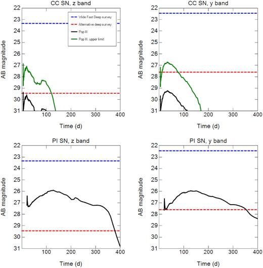
LCs for the brightest CC SN (top panels) and PI SN (bottom panels) in the z and y bands at z = 5.1 and 5.5, respectively. The x-axis is the time in the observer frame τ. In the upper panels the black line is the Pop III CC SN LC and the green line is the LC expected for a Pop I CC SN of equal energy and progenitor mass, which is brighter as discussed in Section 2.1.2. The dashed horizontal lines are the detection limits for the Wide Fast Deep survey (blue) and the alternative deep survey (red) described in Section 3.
The brightest CC SN and PI SN in the z and y bands. Here, z is the redshift at which the SN is brightest in the given filter, mAB is the peak AB magnitude of the event at this redshift, tP is the time in the rest frame at which the SN reaches peak brightness, and μmin is the minimum magnification for the SN to be detected in the LSST WFD survey. μavg is the average magnification of detected SNe. For CC SNe, the first and second numbers for μmin and μavg are for zero- and solar-metallicity SNe, respectively.
| Type | CC | PI | CC | PI |
|---|---|---|---|---|
| Filter | z | z | y | y |
| M⋆ (M⊙) | 15 | 250 | 15 | 250 |
| ESN (foe) | 2.4 | 94 | 2.4 | 94 |
| z | 5.5 | 5.0 | 5.1 | 5.0 |
| tP | 0.8 d | 21.2 d | 5.4 d | 21.2 d |
| mAB | 29.36 | 25.90 | 29.21 | 25.95 |
| μmin | 260/26 | 11 | 510/51 | 25 |
| μavg | 520/51 | 22 | 1000/100 | 50 |
2.3 Cosmic SFRs/SNRs
Cosmic SNRs depend directly on global SFRs and their mass functions. SFRs derived from semianalytical models (e.g. Weinmann & Lilly 2005; Wise & Abel 2005) and numerical simulations over the years have varied by a factor of 200 or more depending on redshift (see e.g. fig. 5 of Whalen et al. 2013a). More recently, simulations using older cosmological parameters have also produced SFRs that are not consistent with current constraints on the optical depth to Thomson scattering by free electrons at high z (τe; Visbal, Haiman & Bryan 2015). To avoid these difficulties we compute Pop II SNRs from cosmic SFRs extrapolated from observations of GRBs, which are used as tracers of early SF (Robertson & Ellis 2012). We apply the Salpeter IMF (Salpeter 1955) to convert these rates to SNRs, adopting the lower limits to the GRB rates to be conservative.
Pop III SNRs were calculated with a semi-analytical model that utilizes a cosmologically representative set of halo merger trees with detailed prescriptions for radiative and chemical feedback on star formation in the haloes (Hartwig et al. 2015; Magg et al. 2016). This model assumes a logarithmically flat IMF (Greif et al. 2011) for Pop III stars, whose masses are randomly sampled over an interval of 1–300 M⊙. We adopt a logarithmically flat IMF because it is commonly assumed in the Pop III star community on the basis of radiation hydrodynamical simulations of primordial star formation (Hirano et al. 2014, 2015). By tracing all the individual randomly generated Pop III stars, the model makes self-consistent predictions for SNRs over the mass range of each explosion type discussed earlier.
SNRs within each explosion type are further partitioned by progenitor masses for which there are LCs. Thus, CC SNRs are divided into the two mass bins from 15–30 M⊙, RPI SNRs are partitioned across nine bins from 90–140 M⊙, and PI SNRs are calculated for five bins from 150–250 M⊙. We show total SNRs for each explosion type as a function of redshift in Fig. 2. As expected, Pop III SNRs taper off with redshift as the universe becomes more chemically enriched, falling off dramatically at z ∼ 5 when metals become present in most of the Universe. In contrast, Pop II SNRs rise over this interval as metals contaminate more and more stars, reaching a peak at z ∼ 2–3 that coincides with the observed peak in cosmic SFR due to galaxy formation.
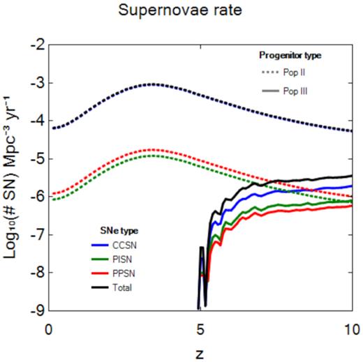
Pop III (solid) and Pop II (dashed) SNRs as a function of redshift, including CC (blue), PI (green), RPI plus PPI (red), and total (black) SNRs. The Pop II CC SNRs are essentially indistinguishable from the total Pop II rates.
2.4 Magnification functions
We take the lenses to be distributed sparsely enough that their areas do not overlap and are thus additive. These magnification areas become less certain at low μ because NFW profiles more accurately represent lensing objects near their cores where densities are high. Our assumption that lensing areas do not overlap also breaks down at low μ, so we only compute magnification areas for μ ≥ 2. For 1 < μ < 2 we logarithmically extrapolate the area from its value at μ = 2 (Section 3.4). This approach does not return the original field of view (FoV) as μ approaches 1 so our maps represent a lower limit to the area on the sky that is strongly lensed. At μ = 1 we simply take the magnified area to be the FoV. At the other extreme, the magnified area falls as μ−2 at large μ for geometrical reasons, so at μ > 100 we take it to be the area at μ = 100 scaled downward by this factor.
We calculate magnification functions for massive galaxies with the Collett (2015) model. The galaxies are assumed to be isothermal ellipsoids with velocity dispersions drawn from the observed velocity dispersion function from SDSS (Choi, Park & Vogeley 2007). We truncate the velocity dispersion function between 50 and 400 km s−1. Like clusters, these lensing galaxies are assumed to be randomly distributed but they are taken to have a constant comoving density out to z = 2. We draw lens ellipticities from the velocity dispersion dependent fit of equation (4) in Collett (2015) and have neglected the effect of compound lensing, which, while rare, can produce extreme magnifications of high-redshift sources (Collett & Bacon 2016). The Collett (2015) model reproduces the galaxy lens samples discovered by the Canada France Hawaii Telescope (CFHT; Gavazzi et al. 2014). The lens population discovered in the Dark Energy Survey (DES; Jacobs et al. 2019) is also broadly consistent with the Collett (2015) forecasts so we take them to be accurate to within a factor of two.
The parameters for both models are listed in Table 2. The mass limits listed for the Collett (2015) model are the masses residing within the Einstein radius. Since the two models cover different ranges in lens mass, the total area that is magnified within the survey area can be approximated by simply summing their respective contributions. The Collett (2015) model produces magnified areas that are somewhat larger than those of Maturi et al. (2014), by up to 50 per cent, but their overall agreement is consistent with the total lensing cross-sections of the two populations being comparable because they have been found to have similar contributions to the optical depth in numerical simulations (Hilbert et al. 2008). Rather than sum the respective PS(μ, zS) of the two models to obtain the total area of the survey area that is lensed, we calculate the number of lensed SNe from each model separately and sum them to obtain the total number, which is equivalent.
Magnification model parameters.
| Maturi | Collett | |
|---|---|---|
| Mass distribution | Sheth–Tormen | Empirical |
| Density profile | NFW | Isothermal ellipsoid |
| Mass range | 1013–1015 M⊙/h | <1013 M⊙ |
| Redshift range | 0.05 < z < 10 | 0.015 < z < 2.0 |
| Maturi | Collett | |
|---|---|---|
| Mass distribution | Sheth–Tormen | Empirical |
| Density profile | NFW | Isothermal ellipsoid |
| Mass range | 1013–1015 M⊙/h | <1013 M⊙ |
| Redshift range | 0.05 < z < 10 | 0.015 < z < 2.0 |
We list the minimum and average magnifications required to detect CC and PI SNe in the y and z bands in the WFD survey in Table 1. At first glance, they are non-linearly dependent on peak AB magnitude in both filters, with Pop III CC SNe requiring much higher magnifications to be observed than their Pop II counterparts. However, the ratios of the magnifications required for zero- and solar-metallicity explosions are consistent with their relative peak magnitudes. In both bands the Pop II CC explosions have peak AB magnitudes that are on average 2.5 lower than peak Pop III CC SN magnitudes at equal energy and progenitor mass, which corresponds to a factor of 10 higher in luminosity. The minimum and average magnifications exhibit similar ratios. Both types of explosions are more easily detected in the z band.
2.5 Lensed SN detection rates
2.6 SN identification
N(z, Δz) is the number of SNe that would appear in a single or stacked observation of the FoV under the assumption that their luminosities remain nearly constant over the exposure time. But they can only be identified as SNe by subtracting two or more exposures of the same FoV, or difference imaging. Objects that appear, disappear, or change in brightness over the time between observations, or cadence Δτ, are tagged as SN candidates. To verify that a candidate actually is an SN, follow-up observations are required. Ideally, spectroscopic measurements of distinctive emission lines could identify the transient as an SN. Alternatively, broad-band follow-up observations could match the LC to a certain SN type. To perform such follow-ups the event must be visible after initial identification, so we discard SNe disappearing between observations. Our SN detections are therefore objects that appear between exposures as well as objects that have changed brightness by more than 25 per cent. As this is an arbitrary threshold, chosen to reflect changes in flux that can be easily detected, we considered a range of thresholds to investigate their effect on our number counts in Section 3.4.
2.6.1 New SNe
For an SN to appear as a new object in the second image it has to brighten between the two images. It could be that the explosion itself takes place in between the two images or that the afterglow brightens between them. If an SN is brighter in the second image, the area in which it is observable in the first image is smaller. The area in which this SN would be detected as an appearing object is therefore the area in which it can be observed in the second image minus the area in which it would have been also observed in the first image. This results in the area of the sky where it would be observed to be flagged as an appearing object.
2.6.2 Evolving SN
2.6.3 Multiple flaggings of the same SN
This result indicates that if a certain region is continuously observed for lensed SNe it is the peak luminosity of the LC that is important to its detection. The peak luminosity produces the largest area in which the SNe can be observed, and at some time during its evolution the SN will be appear as new SN if it falls within this area. Since observations are taken at discrete times there is a risk of one not falling on the peak of the SN, and this possibility is taken into account in our calculation. Lastly, the discretization for computational purposes of the LC is included in our models.
2.6.4 False positives
While a comprehensive procedure for distinguishing z = 5–7 SNe from false positives in the LSST data stream is beyond the scope of this paper, we outline here how it might be done. If an LSST survey in the u, g, r, i, z, and y filters has a cadence of about 30 d, Fig. 1 shows that some CC SNe might appear in every filter (and even more PI SNe may appear because of their extended LCs). No detections in the u, g, and r bands would indicate a redshift >5, which would filter out many low-redshift false positives such as active galactic nuclei (AGNs). If there are multiple observations in the i, z, y filters they can be used to distinguish CC and PI SNe from other false positives. However, if it is necessary to use observations in the i and y filters to identify SNe then the predicted upper limit count declines, as shown in Table 3. Finally, while it is not currently incorporated in our method, another way to reduce false positives in our counts would be to look for the multiple images and time delays associated with the high average magnifications required to detect these events.
Predicted total counts of lensed SNe for the WFD survey from 5 < z < 7 by filter and type.
| Filter | |||
|---|---|---|---|
| SN type | i | z | y |
| Pop II CC (hi) | 43 | 110 | 17 |
| Pop II CC (lo) | 0 | 1 | 0 |
| Pop II PI | 5 | 10 | 2 |
| Pop II IIn | 0 | 1 | 0 |
| Pop II PPI | 0 | 0 | 0 |
| Pop III CC (hi) | 0 | 0 | 0 |
| Pop III CC (lo) | 0 | 0 | 0 |
| Pop III PI | 0 | 0 | 0 |
| Pop III IIn | 0 | 0 | 0 |
| Pop III PPI | 0 | 0 | 0 |
3 RESULTS
3.1 WFD
We show Pop II and III SN detections in the WFD as a function of redshift in Fig. 3 and tabulate total detection rates for each type of explosion from z = 5 to 7 in Table 3. Although the WFD cannot detect unlensed SNe at z ∼ 5–7 at all in the u, g, and r bands and it is too shallow to find them in the i, z, or y bands (see Fig. 1), it could find large numbers of lensed Pop I/II SNe in the z band: ∼1–110 CC SNe depending on their brightness and ∼10 PI SNe, but no PPI SNe. Only a fraction of these events will appear in the y band: ∼2 PI SNe, no PPI SNe, and at most 17 CC SNe. No Pop III SNe will appear in any of the bands due to their low numbers at z < 7, not due to the intrinsic brightness of their explosions.
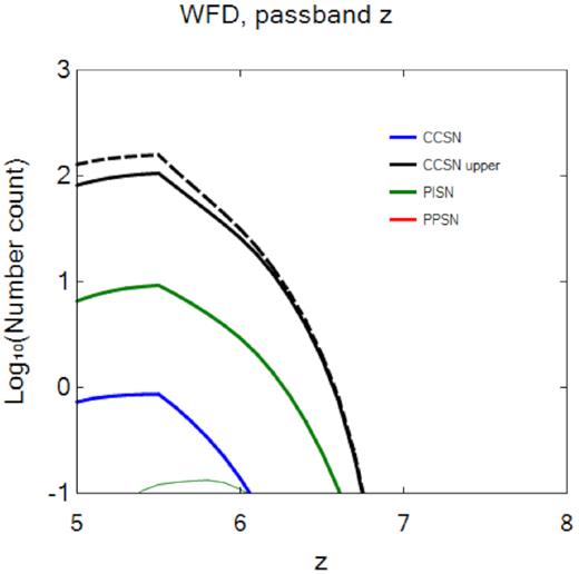
Number of Pop II and Pop III SNe detected per unit redshift in the WFD survey (thick and thin lines, respectively). These SNe are all lensed because the WFD lacks the sensitivity to detect unlensed events. The black dashed line is the predicted number of all explosions when SNe that rebrighten are not rejected as new events. The failure to properly identify such SNe can lead to number counts that are nearly twice the actual values.
It is evident from the black dashed line in Fig. 3 that the failure to reject rebrightening as a spurious event can lead to number counts that are nearly twice the actual values. As noted in Section 2.6.3, variations in the LCs of some SNe can cause them to be detected, fade, and then be detected again when they brighten later, mimicking two new events if they are not properly identified. The breaks in the plots at z ∼ 5.5 are due to Ly α beginning to be redshifted into the filter: at higher redshifts more and more of the radiation from the explosions is scattered by neutral hydrogen so detection rates fall.
3.2 DD
We show the total number of SN detections in a single 10 deg2 DD field as a function of survey depth in AB magnitude in Fig. 4, assuming two observations one year apart. The exposure time required for a given magnitude on the lower axis is noted in red on the upper axis. Most of these events are not lensed because of the low probability of lensing in the relatively small survey area. The few that are lensed can be seen in the CC SN upper plot as the break in slope at AB mag ∼27. The break in slope in the blue CC SN detections at AB mag ∼29 is due to Type IIn SNe.
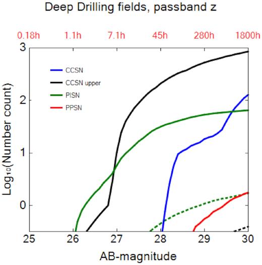
Total number of Pop II and Pop III SNe detected from 5 < z < 7 as a function of observational depth in AB magnitude in the DD survey (thick and thin lines, respectively). On the upper axis is the exposure time necessary to reach the corresponding AB magnitude on the lower axis.
There are larger uncertainties in SN counts at longer exposure times because the luminosity of an event can vary over these times. This is less of an issue with PI SNe because their luminosities evolve more slowly than those of CC SNe, which are dimmer and more rapidly varying. Nevertheless, at the redshifts we consider they are still extended events in comparison to the one to two night explosion peaks of most low-redshift SNe. The time-scales on which the LCs in Fig. 1 evolve suggest that exposure times could be as high as ∼80h (10 d) for CC SNe and 800h (100 d) for PI SNe before serious inaccuracies in the counts would arise. These counts are quite sensitive to survey depth. To detect Pop II CC SNe the DD field must reach AB magnitudes of 27–28, or exposure times of 7.1–45h. This range is derived from the upper and lower limits to the luminosities of CC SNe. To find Pop II PI SNe the DD field must slightly exceed AB mag 26, or a few hours of exposure, while Pop II PPI SNe and Pop III PI SNe require AB magnitudes above 29, or more than 300h of exposure.
3.3 ADS
As shown in Fig. 2, at z ∼ 5–7 most SNe will not be Pop III explosions because most stars will be polluted by metals to some degree by the end of cosmological reionization. Furthermore, Pop III SNe would be difficult to distinguish from Pop II and I explosions of similar energy and progenitor mass because the differences between their spectra are not yet well understood. Nevertheless, at these redshifts some Pop III SNe would be expected. How much LSST survey area and time would be required to detect enough events at z ∼ 5–7 to be statistically confident that some would be Pop III explosions? Here, we consider a variety of survey times and areas in an ADS and the numbers of Pop III SNe they would be expected on average to capture.
Two 640h (80 d) exposures in a single 10 deg2 field one year apart would yield a gain of 6.1 in AB magnitude over the WFD, mAB = 29.5 in the z band. Each exposure is assumed to be a single image in our calculations, and is long enough that the LC of an event could significantly evolve over its duration, which could distort number counts. This is less of an issue for PI SNe because their luminosities evolve relatively slowly after peak but it is more important for CC SNe because they vary more rapidly. However, we use the single exposure approximation as a starting point. We first calculate the number of Pop III SNe that would appear in a 10 deg2 ADS with the total exposure time above. We then vary the survey area while holding this exposure time constant to determine what field and depth would maximize Pop III SN number counts. Larger survey areas here imply more SNe within the FoV but shorter exposures, i.e. more shallow observations, per pointing, so this calculation explores the trade-off between the two.
We show number counts for Pop III SNe by explosion type for the simplest case in which the 640h exposures are carried out in a single 10 deg2 field in Fig. 5. At most one unlensed PI SN is expected from z ∼ 5–6.4 in the z band. CC SN detections are unlikely even at their upper limit in brightness so none will be found at their nominal brightness. The PI SNe that appear in this survey are all of 150–250 M⊙ RSGs. These numbers can be partly understood from Fig. 1. Even with the deeper exposure the unlensed CC SN is only visible for a short time in the z band, and it is much less likely to be lensed because the survey area is so small in comparison to the WFD. On the other hand, PI SNe are visible for much longer times so the ADS can detect them in spite of its small area. Like CC SNe, they will not be lensed because only a fraction of this area will be magnified.
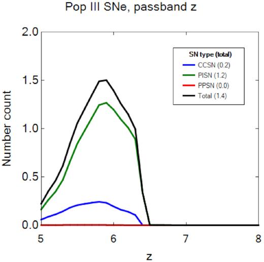
Pop III SN number counts in the z band for two 640h exposures in a single 10 deg2 survey one year apart in the ADS. These are all unlensed events because of the low probability of lensing in this relatively small area. The most likely detections are of PI SNe at z < 6.4. It is unlikely that any Pop III CC SNe will be detected. On average about one SN is expected to be found at z ∼ 6.
In Fig. 6, we show cumulative Pop III SN number counts over z ∼ 5–7 as a function of survey area and AB magnitude limit, again assuming a cadence of one year. They peak at ∼8 in an area of 250 deg2 and mAB = 27.6. PI SNe dominate these counts, ∼ 7 versus ∼ 1 CC SN. We also show PI SN counts by progenitor mass, all of which are RSGs because explosions of BSGs are too faint to be seen. The 250 M⊙ PI SNe will be most numerous (∼ 3) but ∼ 4 of them will be 150–200 M⊙ PI SNe. The number of 250 M⊙ PI SNe increases with survey area, completely dominating the number count above 1000 deg2.
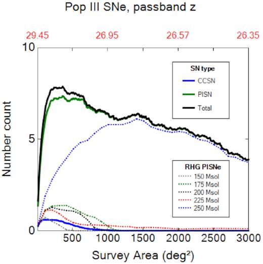
Pop III SN number counts in the z band in the ADS as a function of survey area and sensitivity for a total exposure time of 640h. The lower x-axis is area in deg2 and corresponding AB mag limits are noted on the upper axis in red. The CC SN number counts shown are for their upper limit in brightness.
While the ADS in principle can detect a few Pop III SNe, it is not practical to do so because of the inordinate amount of time that would be required to detect them. Even if these events appear in the LSST data stream it is not currently possible to distinguish them from the much larger number of Pop II SNe LSST would find at z ∼ 5–7 because even Pop III SNe can exhibit metal lines due to rotational or semiconvective mixing in the star prior to death. Lines due to metals could also appear if the ejecta expands through gas enriched by heavier elements, as it likely would at z ∼ 5–7. Although the probability that a given explosion is a Pop III SN rises with redshift, it becomes unambiguous only at z ∼ 20–25, when there has not been sufficient time to pollute the cosmos with metals. The Pop III SN number counts for the ADS shown here refer to the fraction of the total SNe at z ∼ 5–7 that are due to metal-free stars.
3.4 Sources of uncertainty
We summarize the uncertainties in our calculations and their potential impact on our SN number counts in Table 4. The primary source of uncertainty is the rest-frame SNRs, which are derived from cosmic SFRs and the assumed IMF. The global SFRs inferred from GRB observations by Robertson & Ellis (2012) vary by ∼20 per cent at z = 5 to a factor of two to three at z = 7. Since our SN number counts are directly proportional to the SFRs they vary by the same factor in this parameter. We adopted a Salpeter IMF for the Pop II/I stars in our models to obtain conservative counts. If we instead use the more realistic Kroupa IMF we obtain counts that are ∼50 per cent higher. There is a large uncertainty in the IMF of Pop III stars but SN counts in the main survey are dominated by Pop I and II explosions so this uncertainty does not impact the total counts. The ADS is much more sensitive to uncertainties in the Pop III IMF.
Sources of uncertainty in SN counts.
| Type | Impact | On |
|---|---|---|
| SFR/SNR | 20 per cent factor two to three | Pop II |
| IMF | +50 per cent | Pop II |
| Type IIn 1 per cent | 0–10 | CC SN in DD at AB-mag > 28 |
| Type IIn 1 per cent | 0 | CC SN |
| PP SN factor | 0 | PI SN |
| RSG factor 75 per cent | −100 per cent to + 33 per centa | CC SN and PI SN |
| CCSN energy distribution | −100 per cent to +200 per centa | CC SN |
| Detection change threshold (25 per cent) | 0 | WFD |
| Detection change threshold (25 per cent) | 0.01 | ADS |
| ADS cadence if > 1–2 months | 0 | ADS |
| Attenuation Ly α scatter | 100 per cent of Madau | i band |
| Attenuation Ly α scatter | 35 per cent of Madau | z band |
| Attenuation Ly α scatter | 0 | y band |
| Lens Model | −50 per cent to 100 per cent | all |
| Magnification mu 1–2 interpolation | 0 | WFD |
| Magnification mu 1–2 interpolation | 1 | ADS |
These are the lower/upper limits on how the results can vary.
3.4.1 SN type
Since at most 1 per cent of CC SNe are Type IIne and on average only 0.5 Pop II would be found in the WFD, the actual fraction of CC SNe we take to be Type IIn has little impact on our counts predicted for this survey. This is not true of DD fields deeper than AB-magnitude ≳ 28 in which >10 Type IIn are predicted to be found. Here, the uncertainty in ratio of Type IIne to all CC events becomes significant. Less than one PPI or RPI SN will be observed, so the number of 107.5–112.5 M⊙ stars we take to die as PPI events rather than RPI SNe would not alter our counts. We find that only RSG CC and PI SNe will be observed so our predicted number counts are linearly dependent on the fraction of stars that die as RSGs, 75 per cent in our study. At the lower limit of luminosity no CC SN detections are predicted. At the upper limit, the number counts are all due to 25 M⊙ RSG SNe, with the more energetic events dominating the total count. Thus, this count depends on the fractions of SNe assumed to be 0.6, 1.2, or 2.4 foe, which are equal in our study. Essentially all the PI SN detections are 250 M⊙ RSG explosions.
3.4.2 Detection criteria
In our detection criteria, we flag every object whose flux has changed by 25 per cent or more as an SN. Changing this threshold has no effect on the predicted numbers of SNe in the WFD because it only tallies new events because the area on the sky being surveyed never changes. Any new detection at the site of a previous one due to a change in its LC is simply discarded, with no effect on the count. However, the ADS counts evolving sources as new SNe and is therefore sensitive to the threshold. But this effect is small. We find that changing the threshold from 25 per cent to 1 per cent only increases the number count by ∼0.01.
There is a dependence of number count on the cadence, and it can be used to set the actual cadence. Although the cadence of the main survey is already fixed at 27d on average, number counts in the ADS increase until the cadence reaches a few times 10 d and are more or less flat thereafter. Consequently, number counts in the ADS are not sensitive to cadence above 1–2 months. Also, we note that with just two pointings one year apart in DD fields, our number counts could be contaminated by false positives due to AGNs. However, these objects can be disentangled from high-z SNe to some degree because their luminosities are typically higher than those of SNe and fluctuate stochastically by about an order of magnitude over the time-scales that SN LCs evolve. In contrast, SNe brighten and then fade by a larger factor.
3.4.3 Scattering/absorption
We treat attenuation of flux due to Ly α scattering with the model of Madau (1995) at z < 6 and with Gunn & Peterson (1965) for z > 6. The errors in Madau (1995) can be large but λLy α is only redshifted through the i band and |${\sim}35{{\ \rm per\ cent}}$| of the z band at z < 6. The large uncertainties in Madau (1995) therefore have little impact on our results because of the low numbers of counts in the i band and because they only affect part of the z band. High-redshift SNe might be obscured by dust at lower galactic altitudes. However, this will likely have little effect on the number of detections since this region of the sky is not covered by the WFD. There may also be extinction in the host galaxies. This extinction depends on the metallicity. Pop III galaxies are believed to be free of dust, so they would not obscure explosions (Rydberg et al. 2017). Dust in the host galaxies of Pop II SNe may dim them but the extinction is expected to be weak because they are being observed in rest-frame UV. At z ∼ 5–7 the host galaxies also likely have low metallicities and less dust.
3.4.4 Lensing model
For the systemic errors due to the lensing models, we use the factor two, as mentioned in Section 2.4, as an to denote the possible errors in the predicted numbers of SNe.
A source of potentially large uncertainty in our lensing models is the fraction of the sky with 1 < μ < 2 (Section 2.4). The interpolation we use yields a rather severe lower limit because at μ = 1 it returns a lensed area that is just a few per cent of the sky. As a simple test of how robust our counts are with respect to this interpolation we have done it with a second-degree polynomial in the log10–log10 plane as well. As constraints we use f(μ = 1) = 1 and f(μ = 2) = f2, where f(μ) is the fraction of the sky magnified by at least μ. The slope of the interpolation between μ = 2 and μ = 3 is set equal to the derivative of the polynomial.
None of the counts in the WFD change because detections there always require magnifications greater than two, as seen in Table 1. In the ADS the use of this interpolation adds on average only one lensed SN. Although this interpolation is arbitrary, it demonstrates the sensitivity of the counts to the magnification model at 1 < μ < 2. This is true even for CC SNe at their upper limit in brightness, which are not listed in Table 1 but whose minimum magnifications can be obtained from those in the table by dividing them by 10. In the ADS the use of this interpolation adds on average only one lensed SN. Although this interpolation is arbitrary, it demonstrates the sensitivity of the counts to the magnification model at 1 < μ < 2.
Multiple images of SNe behind galaxies and galaxy clusters can confuse SN number counts. The appearance of such images can be separated by weeks because of time delays due to lensing, and because they appear in different regions of the sky they could be mistaken for distinct events. But unlensed explosions do not exhibit multiple images so this phenomenon will have no effect on their number counts. Time delays could boost detections of lensed explosions, but we neglect them because their numbers are expected to be small at low magnifications and because the number of counts that require high magnification are low, so even a relatively large boost would not change them much.
3.5 Other uncertainties
Other factors can alter or reduce our number counts, such as choice of radiation transfer algorithm, other theoretical uncertainties in model spectra, and microlensing of lensed images. These factors can come into play especially in surveys with only nominal predictions of SN counts, such as the 10 deg2 ADS in which only one to two explosions were expected to be found. Borderline number counts such as these are also subject to statistical effects that could reduce the actual yield of lensed Pop III SNe to zero. For example, the |$\sqrt{N}$| statistical error associated with predictions of one to two events yields 1 ± 1 or 2 ± 1.41 detections, which are consistent with zero.
4 CONCLUSIONS
We find that the LSST WFD survey could detect up to ∼110 Pop II CC SNe and ∼10 Pop II PI SNe at z ∼ 5–7, but no Pop III SNe. These are all lensed events because the WFD lacks the sensitivity required to directly detect SNe at these redshifts, even PI SNe. The absence of Pop III SNe in the WFD is due to the much larger numbers of chemically enriched versus pristine stars at this epoch. The large range in Pop II CC SN count (0–110) is due to its highly non-linear dependence on the threshold magnification required for detection and the range of CC SN luminosities over progenitor metallicity. While the uniform cadences we adopted for the WFD introduce some error into our rates, it is subsumed by the uncertainty in cosmic SFR at z ∼ 5–7, which is much higher.
A single 10 deg2 DD survey with two exposures one year apart must reach an AB magnitude >26 to observe Pop II PI SNe at z ∼ 5–7 and >29 to detect Pop III PI SNe. For Pop II CC SNe the depth required is AB mag 27–28. With a deeper exposure (640h) distributed over a 300 deg2 area yielding mAB = 27.6, the ADS could discover ∼7 Pop III PI SNe and ∼1 Pop III CC SN. However, as noted earlier, while some Pop III SNe could appear in the ADS (and in long exposures in the DD), they could not be discriminated from Pop II events at the same redshift. Extremely long times would be required to find them and would not be worth the limited science that could be done with these events.
The relatively small numbers of SNe at z ∼ 5–7 will have to be extracted from the millions of SNe expected at z ∼ 0–1 in the LSST data stream. While a detailed discussion of the methods required to do this are beyond the scope of this paper, we note that after an event is flagged as an SN one can make an initial redshift cut from its Lyman break in one of the filters. If it is still bright enough after discovery by LSST it can then be studied in greater detail with JWST or one of the European Large Telescopes(ELTs). A trigger on the variation of the LC with cadence could also be set, given that high-z SNe LCs will evolve more slowly. But spectroscopic follow-up with the JWST NIRCam or ground-based instruments would still be the best route to determine its redshift. As to whether or not a given event is lensed, one could either look for multiple images of the SN or compare its observed flux to that expected from the template explosion to which it is matched, given its source redshift.
In the long term, observations by JWST and the ELTs at 2–5 |$\mu$|m will be required to find the first SNe in the universe. But wide-field surveys in the H band by Euclid and the Wide Field Infrared Survey Telescope (WFIRST) could extend detections of lensed SNe to z ∼ 15 in the interim and probe the properties of stars in the earliest galaxies. Calculations of lensed SNRs for these missions are now under development.
ACKNOWLEDGEMENTS
We thank Daniel Holz and Matthias Bartelmann for their advice over the course of this project. CER was supported by the European Research Council under the European Community’s Seventh Framework Programme (FP7/2007–2013) via the ERC Advanced Grant ‘STARLIGHT: Formation of the First Stars’ (project number 339177). DJW was supported by Science and Technology Facilities Council (STFC) New Applicant Grant ST/P000509/1 and the Ida Pfeiffer Professorship at the Institute of Astrophysics at the University of Vienna. TC was funded by a University of Portsmouth Dennis Sciama Fellowship. Maturi and MC were partially supported by the Transregional Collaborative Research Centre TRR 33.
REFERENCES
Author notes
Ida Pfeiffer Professor.
