The multiphase gas structure and kinematics in the circumnuclear region of NGC 5728 Free

ABSTRACT

1 INTRODUCTION

Beyond being the some of the most energetic objects in the Universe, active galactic nuclei (AGNs) are thought to play an important role in the evolution of their host galaxies. In particular, large-scale cosmological simulations require feedback from AGNs to reproduce the galaxy population we observe today (e.g. Springel, Di Matteo & Hernquist 2005; Bower et al. 2006; Croton et al. 2006; Nelson et al. 2019). More complete knowledge of the processes that fuel AGNs and the mechanisms through which they provide feedback is then necessary to understand the path galaxies take from being gas rich and star-forming to gas poor and quiescent.

To obtain this understanding however requires dedicated observations that cover a large range of wavelengths and spatial scales to reveal the dominant processes. AGNs only occupy the very centres of galaxies but both streaming gas fuelling the AGNs as well as outflowing gas from AGN driven winds or jets can reach at least several kpc away (e.g. Rupke & Veilleux 2011; Fischer et al. 2013; Cicone et al. 2014; Bae et al. 2017; Baron et al. 2018; Fischer et al. 2018; Herrera-Camus et al. 2019; Kang & Woo 2018; Mingozzi et al. 2019; Bischetti et al. 2019). Furthermore, this gas does not exist in a single phase but rather consists of a mixture of different phases from cold molecular gas to warm ionized gas to hot X-ray emitting gas. Thus to obtain a full accounting of the direct fuelling and feedback of the AGN will need multiple continuum and emission line tracers to probe each phase of the gas.

With the rise of integral field unit (IFU) instruments, large radio interferometers and adaptive optics (AO), it is now possible to study simultaneously the distribution and kinematics of both ionized and molecular gas at the same spatial scales in an efficient manner. For nearby galaxies, this translates to a wealth of information that can span tens of pc to hundreds of kpc, and the kinematics of the gas can further be compared to the stellar kinematics through the analysis of stellar absorption lines to reveal non-circular motions such as radial inflow or outflow. Indeed there has been an increased effort in combining mutliwavelength data to obtain a full view of the conditions and dynamics of gas around AGNs. Recent examples include NGC 5643 (Alonso-Herrero et al. 2018), ESO 428-G14 (Feruglio et al. 2019), ESO 578-G009 (Husemann et al. 2019), NGC 3393 (Finlez et al. 2018), NGC 1566 (Slater et al. 2019), NGC 2110 (Rosario et al. 2019), and zC400528 (Herrera-Camus et al. 2019). These works primarily paired ALMA observations of CO emission with an optical or NIR IFU observation to measure inflow and outflow velocities and gas masses, gas excitation, and bar driven instabilities.

The importance of multiphase observations, in particular for studying AGN feedback, was outlined in Fiore et al. (2017) who compiled and reanalysed data probing AGN driven outflows in the molecular, ionized, and X-ray emitting phase. Their findings revealed strong correlations between the AGN luminosity and outflow velocity, mass outflow rate, and wind momentum for all phases of the gas. However the scaling relations differ depending on the phase resulting in a changing fraction of outflowing gas in one phase that is dependent on the strength of the AGN. The Fiore et al. (2017) scaling relations also do not extend to lower luminosities that are more representative of the larger population of AGNs. It remains to be seen whether they are valid for Seyfert-like AGNs with recent work using dust as a tracer of AGN outflows suggests the relations break down (Baron & Netzer 2019).

Assessing an AGN’s impact on its host galaxy requires measurements of important physical properties of the outflowing gas including the radial extent and the electron density. Without spatially resolved data and lines that accurately trace the electron density, estimates of the mass outflow rate and energetics can be off by orders of magnitude. Revalski et al. (2018a), using high spatial resolution HST imaging and long slit spectra, showed that while global estimates of outflow properties overall agree with spatially resolved estimates, they come with large uncertainties and highly depend on the assumed geometry and density of the system. Only with precise knowledge of the radial extent and gas density will globally averaged mass outflow rates, kinetic luminosities, and momentum rates come close to those obtained from spatially resolved data.

A parallel and equally important focus of studies of nearby AGNs is not how gas is being removed but rather how gas is fuelling the AGN. Many mechanisms have been proposed to extract angular momentum and drive gas to the central supermassive black hole (SMBH) but so far no unique one has been found to explain all observations of AGNs. Instead a range of mechanisms can likely fuel AGNs that depends on the luminosity and morphology of the host galaxy. For low to moderate luminosity AGNs, recent work suggests that gravitational torques produced by non-axisymmetric potentials are efficiently bringing gas down to the inner kiloparsec (e.g. Combes 2003; García-Burillo et al. 2005; García-Burillo & Combes 2012; however also see Sormani et al. 2018). Hydrodynamic simulations show that gas flowing along a bar settles into a nuclear ring, spatially located in or near the Inner Lindblad Resonance (ILR), but further inflow inner to the ring is small without subsequent dynamical instabilities such as another nested nuclear bar (Combes & Gerin 1985; Piner, Stone & Teuben 1995; Maciejewski et al. 2002; Regan & Teuben 2003; Maciejewski 2004). Instead of nuclear rings, nuclear spirals can also form and propagate down to the SMBH given a higher gas sound speed (Maciejewski et al. 2002; Maciejewski 2004) and indeed nuclear spirals have been found in many galaxies hosting an AGN (Pogge & Martini 2002; Martini et al. 2003; Prieto, Maciejewski & Reunanen 2005; Davies et al. 2009, 2014). Since cold molecular gas is the fuel for AGNs, it makes sense to turn to observations of CO line emission, a primary tracer for molecular gas, to detect and measure the structure and instabilities bringing gas to the SMBH.

1.1 NGC 5728

NGC 5728 is a nearby SAB(r)a galaxy (D = 39 Mpc, 1 arcsec = 190 pc), with a Compton thick, Seyfert 2 nucleus (Veron 1981; Phillips, Charles & Baldwin 1983). The bolometric luminosity of the AGN is 1.40 × 10⁴⁴ erg s⁻¹ where we have converted the absorption corrected 14–195 keV X-ray luminosity from the Swift Burst Alert Telescope, L_X = 2.15 × 10⁴³ erg s⁻¹ (Ricci et al. 2017), into L_Bol using the relation from Winter et al. (2012). Its primary characteristics include a large stellar bar (R ≈ 11 kpc, P.A.  = 33°; Schommer et al. 1988; Prada & Gutiérrez 1999) which is surrounded by a ring of young stars, a circumnuclear star forming ring (R ≈ 800 pc; Schommer et al. 1988; Wilson et al. 1993), and extended ionization cones (R ≈ 1.5 kpc, P.A.  = 118°; Schommer et al. 1988; Arribas & Mediavilla 1993; Wilson et al. 1993; Mediavilla & Arribas 1995). Rubin (1980) was the first to study the ionized gas kinematics finding that while at large radii the gas displayed normal rotation, the central regions showed strong non-circular motion as well as double-peaked emission lines. Over the years much discussion ensued over the physical explanation of the non-circular motion and double-peaked emission lines with radial outflow (Rubin 1980; Wagner & Appenzeller 1988; Arribas & Mediavilla 1993; Mediavilla & Arribas 1995) and radial inflow due to the bar (Schommer et al. 1988) the primary choices. van Gorkom et al. (1983) and Schommer et al. (1988) also found extended 6 and 20 cm radio emission spatially coincident with the ionization cones suggesting the presence of a jet. Further complicating interpretations was the finding of a strong isophotal twist (ΔP.A. ≈ 60°) in the central ≈5 arcsec from NIR imaging that suggested the presence of a secondary nuclear bar.

This secondary nuclear stellar bar was thought to potentially be the driving mechanism to bring gas from the circumnuclear ring to the SMBH. However, Petitpas & Wilson (2002) found no significant nuclear molecular gas bar coincident with the stellar bar based on spatially resolved CO (1–0) data. Instead they note a double-peaked morphology of the CO emission that straddles the centre but is perpendicular to the ionization cones and suggest that the NGC 5728 might have experienced a recent minor merger that could cause the off-centre CO emission.

All of these intriguing components contained with NGC 5728 make it an ideal system to study the fuelling and feedback of AGNs. In this paper, we report on a combined analysis of recent Atacama Large Millimeter/submillimeter Array (ALMA), Very Large Telescope (VLT) MUSE, and VLT/SINFONI observations that jointly probe the morphology and kinematics of the stars, cold molecular gas, hot molecular gas, and warm ionized gas on both large and small spatial scales. Recently, Durré & Mould (2018, 2019) studied NGC 5728 using both the MUSE and SINFONI data sets. Much of our conclusions and interpretation are consistent, but we will note where we disagree and where their analysis enhances ours. Throughout this paper, we assume a Λ cold dark matter cosmology with H₀ = 70 km s⁻¹ Mpc⁻¹ and Ω_M = 0.3.

2 OBSERVATIONS, DATA REDUCTION, AND ANALYSIS METHODS

2.1 SINFONI observations

NGC 5728 was observed by VLT/SINFONI (Eisenhauer et al. 2003; Bonnet et al. 2004) as part of the Luminous Local AGN with Matched Analogues (LLAMA) programme (Davies et al. 2015), a volume-limited survey of nearby X-ray selected AGNs with SINFONI and XSHOOTER. Within this programme, all targets were observed by SINFONI using the H + K grating (1.4–2.5 |$\mu$|m) and AO mode providing integral field spectroscopy with spectral resolution R ∼ 1500 over a roughly 3 arcsec × 3 arcsec field of view (FOV). A standard Object-Sky-Object observation sequence was used with each integration lasting 300 s and the object exposures dithered by 0.3 arcsec. Observing blocks for NGC 5728, under programme ID 093.B-0057 (PI R. Davies), were carried out on the nights of 2015 February 23, March 06, May 09, June 04, and June 25 resulting in 25 Object integrations and 12 Sky integrations for a total on-source time of 125 min.

The raw SINFONI data were reduced using the custom reduction package spred (Abuter et al. 2006) which performs all the standard reduction steps needed for near-infrared spectra as well as additional routines necessary to reconstruct the data cube. We further applied the routines mxcor and skysub (Davies 2007) to improve the subtraction of OH sky emission lines and lac3d, a 3D Laplacian Edge Detection algorithm based on lacosmic (van Dokkum 2001), to identify and remove bad pixels and cosmic rays. Telluric correction and flux calibration were carried out using B-type stars. Finally, we also corrected for differential atmospheric refraction, a wavelength-dependent spatial offset due to the atmosphere, using a custom procedure described in Lin et al. (2018).

The final SINFONI data cube covers a FOV of 3.5 arcsec × 3.7 arcsec with a pixel scale of 0.05 arcsec. With AO, we achieved a point spread function (PSF) full width at half-maximum (FWHM) of 0.15 arcsec based on Gaussian fitting of the unresolved continuum nuclei from the AGN in the LLAMA sample. This translates to a physical spatial resolution of 28 pc over a physical FOV of 660 pc × 700 pc.

2.2 MUSE observations

MUSE is a second-generation VLT instrument consisting of 24 IFUs that span the wavelength range 4650–9300 Å (Bacon et al. 2010). We downloaded archival MUSE data of NGC 5728 from the MUSE-DEEP collection, an ESO Phase 3 data release that provides fully reduced, calibrated, and combined MUSE data for all targets with multiple observing blocks. The original observations were performed over two observing blocks on April 3 and June 3, 2016 for programme ID 097.B-0640 (PI D. Gadotti), and were carried out in seeing limited Wide Field Mode that results in a 1 arcmin × 1 arcmin FOV sampled with a pixel scale of 0.2 arcmin. The total exposure time for the combined MUSE cube is 79 min and Gaussian fitting of a foreground star within the FOV show a PSF FWHM of 0.62 arcsec. The MUSE data cube thus covers an 11.3 kpc square region with a spatial resolution of 177 pc at the distance of NGC 5728.

Fig. 1 shows a three-colour gri image of NGC 5728 from the MUSE cube. As seen in the HST imaging in Fig. 2, the MUSE observation covers a large portion of the large-scale bar which contains long dust filaments and a blue circumnuclear disc/ring. In the right-hand panel, we highlight strong [O iii] and H α emission by using a simple narrow-band filter for the blue and green colours of the image while the red colour is from the i band.

Figure 1.

Left-hand panel: Three-colour gri image obtained by integrating the MUSE cube between wavelengths of 4800–5830 Å for g band, 5380–7230 Å for r band, and 6430–8630 Å for i band. Right-hand panel: Three-colour [O iii] (blue), H α (green), i band (red) image using a narrow band filter to highlight [O iii] (5028–5095 Å) and H α emission (6578–6664 Å).

Open in new tabDownload slide

Figure 2.

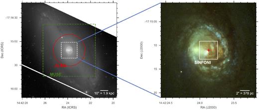
NGC 5728 as observed by HST/WFC3. The left-hand panel is a greyscale image of only the F814W observation to highlight the primary bar and bright circumnuclear region. The right-hand panel is a three colour zoom-in of the region outlined by the white dotted box in the right-hand panel. Red, green, and blue colours are from the F814W, F438W, and F336W filters. In the left-hand panel, the green dashed line indicates the FOV of the MUSE observation while the red circle indicates the FOV of the ALMA observation. The white box in the right-hand panel indicates the FOV for the SINFONI observations and the red cross shows the position of the AGN from VLBI (see Section 2.5). In both panels, North is up and East is to the left.

Open in new tabDownload slide

2.3 ALMA observations

ALMA observed NGC 5728 on May 15, 2016 as part of project 2015.1.00086.S (PI N. Nagar) for a total on-source time of 29 min in the C36-3 configuration resulting in an angular resolution of 0.56 arcsec × 0.49 arcsec (PA = −79.4°) in Band 6. This observation was part of an ALMA programme to map CO (2–1) in the nuclear regions of seven local AGNs (Ramakrishnan et al. 2019). The spectral set-up was designed to centre one of the spectral windows on the redshifted CO (2–1) emission line (ν_rest = 230.538 GHz) for NGC 5728.

We used the Common Astronomy Software Applications package (casa; McMullin et al. 2007) to process the data. Within the tclean routine, we applied Briggs weighting with robust  = 0.5 to reproduce the data cube at 2.54 km s⁻¹ velocity resolution and a peak residual (parameter threshold) of 2.5 mJy. All resulting data cubes were primary beam corrected and a 1.3 mm continuum image was extracted by combining and integrating the remaining three spectral windows without the CO (2–1) line.

2.4 HST observations

The final data set we primarily use for this work is archival multiband HST imaging. HST observed NGC 5728 in the F336W, F438W, F814W, and F160W bands with the Wide Field Camera 3 instrument as part of programme 13755 (PI J. Greene). We downloaded the standard pipeline reduced images from the Mikulski Archive for Space Telescopes.¹

Fig. 2 shows the F814W (left) with a three-colour zoom-in of the circumnuclear region that combined the F814W, F438W, and F336W images as red, green, and blue colours, respectively. The larger scale F814W image also has overplotted the FOV’s of the ALMA (red circle) and MUSE (green box) data sets. Both ALMA and MUSE cover a large portion of the primary bar and the entire circumnuclear region. The FOV of the SINFONI cube (white box) is overplotted on the three colour zoom-in that shows we are probing the very inner regions of NGC 5728. The combination of all of these data sets allow us to consistently trace gas and structure from several kpcs down to tens of pc as well as the interaction between the host galaxy and the central AGN.

2.5 Astrometric alignment and AGN position

To ensure all of the data sets are registered to a common coordinate system, we implemented the following procedure. Luckily at least one bright foreground star lies within the FOV of every HST image and the MUSE cube. Starting with the F336W, F438W, and F814W HST images, we matched the bright stars to GAIA DR2 sources (Gaia Collaboration 2018). To make corrections, we simply updated the WCS parameters by applying small pixel shifts until the positions matched between the images and the GAIA DR2 values. These corrected HST images were then used to correct both the NICMOS F160W image and the MUSE cube, again by applying pixel shifts until the locations of the stars in common matched.

For the SINFONI cube, no foreground stars appear in the FOV, therefore we first produced an H-band continuum image from the cube and used it to match distinct features between it and the HST F160W image. In particular, we aligned the brightest pixel in the SINFONI H-band continuum image with the brightest pixel in the HST F160 image and then checked to ensure other features such as the nuclear dust lane were aligned as well. This gives us an astrometric accuracy of ≈0.25 arcsec (i.e. the angular resolution of HST at 1.6 |$\mu$|m) between SINFONI and the rest of the data sets. Finally, we did not apply any corrections to the ALMA data given the high astrometric accuracy inherent in radio interferometric observations.

For the position of the AGN, we used VLBI observations from The Megamaser Cosmology Project (Kuo, private communication). The coordinates of the AGN are RA = 14:42:23.872 and DEC  = 17:15:11.016 with an accuracy of a few tens mas. The position is shown in the right-hand panel of Fig. 2 as a red cross and will be used as the reference point for all following figures. This position matches very well both the peak of 1.3 mm continuum emission from ALMA (see Fig. 3) as well as the peak of the warm molecular gas traced by H₂ (1–0) S(1) emission from SINFONI (see Fig. A3).

Figure 3.

Results of emission line fitting for the inner 8 x 8 arcsec region of NGC 5728 using a single Gaussian component. The top row shows the integrated flux (left), velocity (middle), and dispersion (right) for CO (2–1) with the black contours plotting the 2σ, 5σ, 10σ, 20σ contours of the 1.3 mm continuum. The middle and bottom rows show the flux, velocity, and dispersion for H α and [O iii], respectively. The black crosses in all panels show the location of the AGN from VLBI (see Section 2.5).

Open in new tabDownload slide

2.6 Spectral fitting

2.6.1 Continuum fitting and subtraction

The data reduction for the ALMA cube includes already a continuum subtraction however both the SINFONI and MUSE cube contain significant continuum signal. To remove the continuum as well as stellar absorption features, we use the Penalized Pixel-Fitting² (ppxf) routine (Cappellari & Emsellem 2004; Cappellari 2017) together with the latest (v11.0) single stellar population (SSP) models based on the extended MILES stellar library (E-MILES; Vazdekis et al. 2016). We chose the models produced from the Padova 2000 stellar isochrones with a Chabrier initial mass function (Chabrier 2003). The SSP models range from stellar population ages of 63 Myr to 14.13 Gyr spaced logarithmically and six metallicities between −1.71 and 0.22.

For the MUSE cube, both to reduce the computation time and improve the signal-to-noise (S/N) ratio in the outer regions, we chose to utilize Voronoi binning before running pPXF. We used the method from Cappellari & Copin (2003) and the voronoi_2d_binning³ Python routine to bin the MUSE cube such that each bin contains a minimum S/N in the continuum of 20.

Each binned or single MUSE and SINFONI spaxel was fit with ppxf. For the MUSE spectra, we used the full range of metallicities and stellar population ages but we also incorporated regularization to better interpret the best-fitting metallicities and ages since the fitting of galaxy spectra is an ill-posed problem (Cappellari 2017). For the SINFONI spectra, because they only cover the near-infrared and are relatively insensitive to young stellar population ages, we only fit using models with ages of 0.1, 0.5, 1.0, 5.0, 10.0, and 14.1 Gyr. We also did not use regularization because our only concern for the SINFONI cube is the removal of the continuum and determination of the stellar kinematics. Because both the MUSE and SINFONI spectral resolutions are only moderate, we only fit for the stellar velocity and velocity dispersion. We also included an additive fourth degree polynomial in the fit to model any emission from the central AGN. To create the continuum-subtracted MUSE cube, we renormalized the best-fitting binned spectra to the median continuum level of each individual spectrum before subtraction. Fig. 4 shows the results of our ppxf fits for the MUSE cube.

Figure 4.

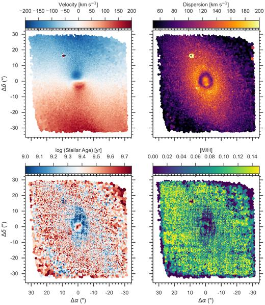
Results from fitting the MUSE cube with ppxf. The top row plots the stellar velocity (left) and dispersion (right). The bottom row plots the mean light-weighted stellar population age (left) and mean light-weighted metallicity (right). In all frames, North is up and East is to the left.

Open in new tabDownload slide

2.6.2 Emission line fitting

To measure the bulk distribution and kinematics of the molecular and ionized gas in NGC 5728, we fit single Gaussians to the relevant emission line tracers of the gas. In particular, we fit the CO (2–1) line (ν_rest = 230.538 GHz) in the ALMA cube; the H β, [O iii] doublet, [O i], [N ii] doublet, H α, and [S ii] doublet lines in the MUSE cube; and the [Fe ii]λ1.64 |$\mu$|m, [Si vi], H₂ (1–0) S(1), and Brγ lines in the SINFONI cube. This set of lines represent the strongest emission lines observed in nearby galaxies and AGNs and provide diagnostic power into the state of gas in a range of phases from cold molecular gas [CO (2–1)] to warm molecular gas [H₂ (1–0) S(1)] to hydrogen recombination lines (H β, H α, Br γ) and forbidden lines ([O iii], [O i], [N ii], [S ii], [Fe ii], [Si vi]) from ionized gas in a range of ionization levels.

For each line, we cut out the relevant sections of the continuum-subtracted spectra that contain the single line or multiple lines in the case of the [O iii] doublet, H α and [N ii] blended region, and [S ii] doublet. We fixed the velocity and velocity dispersion to be the same for all doublets and fixed the intensity ratio to the expected theoretical value of 3 for the [O iii] and [N ii] doublets. For the fit of the [Si vi] line, we also included Gaussian components for the nearby H₂ (1–0) S(3) and Br δ lines. As an estimate of the local noise around each line, we measured the root mean square (RMS) of the line-free regions. Using the RMS, we produced 100 simulated spectra for every emission line by randomly perturbing the original spectra assuming a Gaussian distribution with a standard deviation equal to the RMS. Each of the simulated spectra were fit in the same way as the original spectra and uncertainties on the integrated flux, velocity, and velocity dispersion were calculated from the standard deviation of the best-fitting values from the simulated spectra. Finally, all velocity dispersions derived from MUSE and SINFONI data were corrected for instrumental broadening. For lines from MUSE, we assumed an instrumental dispersion of 49 km s⁻¹ for lines in the [O iii] region and 71 km s⁻¹ for lines in the Hα region based on the spectral resolution curve as a function of wavelength in the MUSE User Manual.⁴ For SINFONI, we assumed an instrumental dispersion of 65 km s⁻¹ based on the width of OH sky lines. Figs A1, A2, A3, and A4 show the results of our single Gaussian fitting for all of the emission lines studied in this paper over the full FOV for each instrument. Fig. 3 shows the results for CO (2–1), H α, and [O iii] zoomed into the central 10 arcsec x 10 arcsec.

3 RESULTS

3.1 Large scales and the primary bar

We begin our investigation of NGC 5728 with the largest scales. As mentioned in Section 1.1, NGC 5728 is characterized on large scales by a primary bar surrounded by a ring of young stars. Continuum emission in general is elongated from the NE to the SW and the MUSE three-colour image (Fig. 2) shows bluer emission encircling the inner, redder bar. These bluer emission regions in the large ring are also spatially coincident with clumps of H α emission indicating recent star formation.

In the top left-hand panel of Fig. 5, we show in both colour and contours the HST F160W image which traces emission from older stars. Again, on the largest scales we observe primarily the large bar with the P.A. of the bar plotted as the white line, however towards smaller radii the stellar distribution becomes more and more spheroidal with the major axis shifting to more N–S. This is also the P.A. for the stellar kinematic major axis as shown in Fig. 4 as well as the photometric major axis for the main disc that the bar lives within (Schommer et al. 1988). Prada & Gutiérrez (1999) observed this isophotal twisting as well in large I-band imaging and attributed it to the increasing influence of the central bulge. This would further make sense given the increasing stellar velocity dispersion which rises to ∼170 km s⁻¹ before dropping at the circumnuclear ring (Fig. 4, top right-hand panel) as well as having a relatively old mean age of ∼5 Gyr compared to both the larger main ring and circumnuclear ring which show ages of ∼1 Gyr (Fig. 4, bottom left-hand panel).

Figure 5.

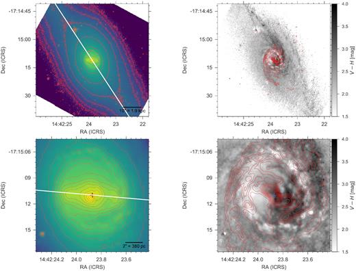
Large scale and circumnuclear zoom-ins of the H-band imaging and V−H dust maps produced from F160W (H) and F438W (V) HST observations. The red contours in the left-hand panels trace the continuum image to better outline the structure while the red contours in the right-hand panels plot the CO (2–1) emission from ALMA. The white line in the top left shows the major axis of the large scale bar and in the bottom left the major axis of the nuclear stellar bar taken from the literature (Schommer et al. 1988; Prada & Gutiérrez 1999).

Open in new tabDownload slide

Roughly straight dust lanes can also be seen in Figs 1 and 2 running the length of the bar with the more prominent dust lane occurring in the northern half and indicating that the west side of the galaxy is the near side (Schommer et al. 1988). To further enhance and highlight the dust lanes, we show in the top right-hand panel of Fig. 5 a V−H map constructed from the F438W and F160W HST images. Areas with high extinction would have large V−H values and appear dark in the map. Indeed the northern dust lane reveals itself as a dark band extending from the NE to the circumnuclear region. We also plot on top of the V−H map contours showing the location of CO (2–1) emission. Interestingly, the northern dust lane lacks strong CO emission and it is instead the southern dust lane that appears as a single spiral arm connecting to the circumnuclear ring. This morphology is consistent with the observations of CO (1–0) emission from Petitpas & Wilson (2002) however they attribute the southern arm as potentially due to a larger ring structure or evidence of a past merger event. Instead it is quite clear within our data sets that it is associated with a fainter dust lane on the far side of the galaxy. It is unclear however why CO (2–1) is missing in the northern dust lane. It is possible that molecular gas here is more diffusely distributed over larger scales that were resolved out of the interferometric observations.

As hydrodynamic simulations show (e.g. Athanassoula 1992; Maciejewski et al. 2002), two straight dust lanes are expected to appear along the bar major axis due to the formation of principal shocks which compress the gas and dust. This occurs due to the gradual shifting of the gas orbits from the x₁ family (i.e. parallel to the bar major axis) to the x₂ family (i.e. perpendicular to the bar major axis). As gas crosses these shocks, it loses angular momentum resulting in inflow towards the centre (e.g. Athanassoula 1992; Maciejewski et al. 2002). As we will show in the next section, we do observe kinematic signatures of inflow at the locations where the dust lanes connect to the central circumnuclear ring strongly suggesting that gas is being driven from the outer disc to the circumnuclear region via the bar. Assuming the gas in the bar is rotation dominated it is expected to settle into a ring (e.g. Piner et al. 1995) or nuclear spiral (Maciejewski et al. 2002; Maciejewski 2004).

3.2 The circumnuclear ring

As many others have before we observe a central circumnuclear ring within the central ≈1.3 kpc in projected radius. Multiple tracers highlight this structure through both their emission and kinematics.

Both the HST and MUSE continuum imaging show a distinct ring of clumpy, blue emission indicative of young hot stars. This is confirmed in the bottom left-hand panel of Fig. 4 which shows the mean light-weighted stellar age. The circumnuclear ring outlined by blue continuum emission also has a distinctly younger mean light-weighted stellar age (1 Gyr versus 5 Gyr) compared to the surrounding region. This fits with the LLAMA finding that on average AGNs show a significant young (<30 Myr) stellar population within the central few hundred parsecs compared to inactive galaxies based on stellar population modelling of high spectral resolution VLT/X-Shooter spectra (Burtscher et al., in preparation). Further, Riffel et al. (2009b) found a significant population of intermediate age stars in stellar population modelling of NGC 5728 using a NIR IRTF spectrum. The stars in the ring further show evidence for lower metallicity which could be an indication that the increased nuclear activity is due to a recent minor merger.

The circumnuclear ring is further revealed kinematically in the stars via strong circular rotation and a drop in velocity dispersion (Fig. 4, top row). While on large scales the stellar velocity peaks at the edge of the FOV and with a P.A. ∼ 0°, there is a clear kinematically decoupled component with velocity peaks at ∼4 arcsec (760 pc) radius and a P.A. ∼ 10°. The dispersion map shows the ring as a ring of decreased velocity dispersions compared to the surrounding regions (70 km s⁻¹ versus 170 km s⁻¹) which spatially corresponds to the ring of younger mean stellar ages. The reduced velocity dispersions can be explained as the primary stellar population not yet thermalizing out of their birth clouds and still moving with regular rotation. These so-called dispersion ‘drops’ have routinely been used in long slit observations of nearby galaxies as markers of nuclear star formation (e.g. Emsellem et al. 2001) .

All of the stellar tracers suggest recent star formation so there should be large amounts of both molecular gas from which the stars were born out of and ionized gas from photoionization by the young stars. Indeed, Fig. 6 shows that exactly where we find the ring of lowered velocity dispersions, we also observe a strong ring of CO (2–1) emission as well as a ring of H α clumps outlining the star forming H ii regions.

Figure 6.

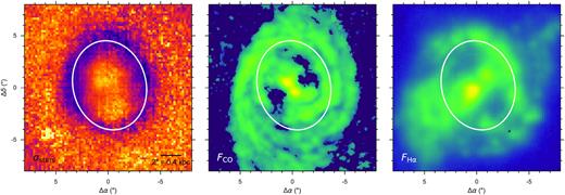
Comparison between the stellar velocity dispersion (left), CO (2–1) flux (middle), and H α flux (right). The white ellipse plots the location of the lowered stellar velocity dispersion in each of the panels to the show the spatial correspondence between the decreased stellar dispersion and the rings of molecular gas and ongoing star formation. Colours in each panel are the same as what is shown in Figs 4 and 3.

Open in new tabDownload slide

The white ellipse plotted in Fig. 6 was chosen to directly follow the ring of lowered stellar velocity dispersion. The parameters of the ellipse have a P.A. of 14°, a semimajor axis 822 pc and an axial ratio (b/a) of 0.8. If we make the assumption that the ring is intrinsically circular then the inclination is related to the axial ratio through cos (i) = b/a. This leads to an estimate of the inclination of ≈37° which is more face-on compared to the large scale photometrically determined inclination of 48–55° (Schommer et al. 1988; Davies et al. 2015). This could be due to our assumption of circularity, since its possible the stars in the ring are on elliptical x2 orbits associated with the large scale bar. These rings of young nuclear star formation associated with low-velocity dispersions seem to be a common characteristic of local Seyfert galaxies as many studies using IFU data have found them within the central kpc (e.g. Riffel et al. 2010, 2011; Diniz et al. 2017; Dametto et al. 2019)

3.2.1 Gas excitation

The MUSE and SINFONI IFU cubes allow for us to spatially resolve the distribution of emission line ratios and assess the dominant mechanism for gas excitation. Gas excitation mechanisms can be identified using popular line ratio diagrams with specific thresholds or demarcations that separate between the different mechanisms which include photoionization by a central AGN, ionization by UV photons from H ii regions, and low-ionization nuclear emission line regions (LINER).

Fig. 7 plots the three standard excitation diagrams (Baldwin, Phillips & Terlevich 1981; Veilleux & Osterbrock 1987) for individual spaxels in NGC 5728. The circumnuclear region of NGC 5728 is dominated by gas photoionized by the AGN, as indicated by the yellow to red colours. The AGN-dominated region further follows the bicone shape of the strong [O iii] emitting region. H ii regions instead follow a clear ring-like structure, encircling the bicone and tracing the ring-shaped emission seen in H α, the three colour HST image, and the molecular gas distribution that is indicated by the white ellipse in the bottom row of Fig. 7. All of this definitively points to strong star formation occurring within the circumnuclear ring.

Figure 7.

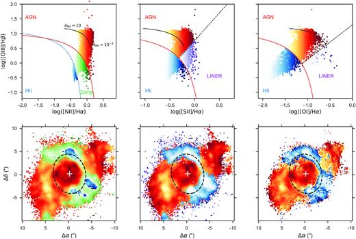
Spatially BPT maps of NGC 5728 derived from emission line fitting from the MUSE cube. The top row plots the BPT line ratio diagrams with each dot representing a single spaxel. To be included in the diagram, the corresponding emission lines had to be detected with S/N > 3. Points are colour-coded according to their location with respect to the Kauffmann et al. (2003, blue dashed), Kewley et al. (2001, red solid), and Kewley et al. (2006, black dashed) classification lines. The black solid lines plot the expected line ratios from Binette, Wilson & Storchi-Bergmann (1996) for an increasing ratio of the solid angle subtended by matter bounded and ionization bounded clouds (A_M/I). The panels in the bottom row show the spatial location of each of the points coloured by their location in the corresponding top row panels. The black dashed ellipses outline the location of the circumnuclear ring seen in Fig. 6.

Open in new tabDownload slide

One interesting feature seen in the excitation diagram is a horizontal ‘spike’ at high [O iii]/H β ratios and pointing towards lower [N ii]/H α, [S ii]/H α, and [O i]/H α ratios. Within each of the diagnostic regions, we shaded the spaxels from light to dark based on the [N ii]/H α, [S ii]/H α, or [O i]/H α line ratio value. In the maps we can then see that the horizontal ‘spike,’ indicated by yellow colours, is primarily occurring in a narrow region on the SE side of the circumnuclear ring and coinciding with where the ring intersects the AGN bicone.

This feature has been seen recently in other nearby AGN with spatially resolved line ratio maps. Mingozzi et al. (2019), using MUSE data for the MAGNUM survey, explained these line ratios as tracing the ratio of the solid angle subtended by matter bounded and ionization bounded gas clouds (A_M/I) as first put forth in Binette et al. (1996). In short, matter bounded clouds are optically thin throughout the entire cloud to the ionizing radiation field while ionization bounded clouds are optically thick and absorb all of the incident ionizing radiation. If matter bounded clouds dominate the solid angle we would expect more emission from high-ionization lines compared to low-ionization ones and vice versa if ionization bounded clouds dominate.

However, we can also explain this feature by an increase in the ionization parameter. Baron & Netzer (2019; BN19) developed a simple method for measuring the ionization parameter using the [O iii]/H β and [N ii]/H α line ratios (see equation 2 of BN19). The main assumption is only that the gas is photoionized by an AGN. Therefore, we calculated the ionization parameter, U, as a function of radius towards the SW using a series of annular sections described Appendix  B and shown in Fig. B3.

Fig. 8 shows the radial profile along the bicone of both [N ii]/H α and U. Indeed, exactly where we observe a decrease of [N ii]/H α, the ionization parameter significantly increases. While both a change in A_M/I and a change in U can explain the horizontal ‘spike’ in the line ratio diagrams, we choose the simpler increase in U model as our explanation. This would be consistent with an interpretation that this region is where the NLR bicone is intersecting the lower density circumnuclear ring since U and gas density are inversely related.

Figure 8.

Radial profile towards the SW along the bicone of both the [N  ii]/H α line ratio and the ionization parameter, U. Radii have not been corrected for inclination and are simply the projected radius from the AGN.

Open in new tabDownload slide

3.2.2 Molecular gas mass

To calculate a molecular gas mass, we must assume a value for |$\alpha _{\scriptscriptstyle \rm CO}$|⁠, the conversion factor from |$L^\prime _{\rm CO}$| to |$M_{\rm H_{2}}$|⁠. For this work, we use |$\alpha _{\scriptscriptstyle \rm CO} = 1.1$| M_|$\odot$| pc⁻²/(K km s⁻²). This is the value found for the central regions of nearby galaxies, likely due to the increased pressure and/or turbulence (Sandstrom et al. 2013). Using this, we find a total molecular gas mass within the central ∼1 kpc of NGC 5728 to be 1.3 × 10⁸ M_|$\odot$|.

This total mass matches well with that found in Rosario et al. (2018) who found a molecular gas mass of 10^8.53 M_|$\odot$|. Our value is 40 per cent of theirs, however the Rosario et al. (2018) measurement is based on an JCMT observation with a beam size of 20.4 arcsec compared to the 6.5 arcsec aperture used here. This seems to be an indication that about 60 per cent of the total molecular gas is on scales larger than 1 kpc given the largest angular scale of the ALMA observation was 5.34 arcsec. We tested whether convolving the ALMA cube to the JCMT beam and integrating over a larger aperture increased the measured molecular mass but did not find any change, an indication that diffuse flux was resolved out due to the lack of short spacings during the ALMA observation.

3.2.3 Disc modelling

Kinematically, all three tracers (stars, molecular gas, and ionized gas) show strong signs of circular rotation (see Figs 4 and 3). Therefore, we can fit the velocity fields with a model of rotation to better constrain the inclination and dynamical mass driving the rotation.

We first fit both the CO (2–1) and stellar velocity fields using an updated python version of dysmal (Davies et al. 2011), now called dysmalpy, an MPE developed software package for modelling the dynamics of galaxies. dysmalpy works by first simulating the mass distribution of a galaxy and populating a three-dimensional cube with the corresponding physical velocities. After rotating and inclining the galaxy to match the preferred line of sight, the physical 3D cube is integrated along the line of sight to produce an observed ‘IFU’ cube which is finally convolved with both a PSF and line spread function. In this way, we account for all instrumental effects including beam smearing. These simulated cubes can then be used to compare and fit against observed data using either standard non-linear least squares or a Markov chain Monte Carlo (MCMC) algorithm with emcee (Foreman-Mackey et al. 2013).

We assumed a thin exponential disc mass distribution parametrized by the total dynamical mass (M_dyn) and the effective radius (r_eff) within which the enclosed mass is one-half of M_dyn. The inclination of the disc (i_disc) and the position angle (P.A._disc) were also left as free parameters in the fitting. For the CO (2–1) model we fixed the centre by eye because we also masked out the inner 2.5 arcsec due to the presence of the non-circular motion described below. For the stellar velocity field we allowed the centre to vary between  +/−5 pixels in both the x and y direction. We ran MCMC with 100 walkers for 100 burn-in steps and 400 sampling steps to determine the best-fitting parameters and uncertainties from the sampled posterior distribution using the median and the 16th and 84th percentiles.

Fig. 9 shows the results of our fitting. For the molecular gas, we find a best-fitting |$\log M_{\rm dyn} = 10.372^{+0.002}_{-0.001}$| M_|$\odot$|, |$r_{\rm eff} = 537^{+2}_{-2}$| pc, |$i_{\rm disk} = 43.3^{\circ +0.1}_{-0.1} $|⁠, and P.A.|$_{\rm disk} = 14.01^{\circ +0.04}_{-0.03}$|⁠. We note that the very small errors on the model parameters only incorporate the statistical uncertainties and thus are more reflective of the high S/N and high spectral resolution of the ALMA data. These results are also consistent with those found using the same data in Ramakrishnan et al. (2019). For the stellar velocity field, we find a best-fitting |$\log M_{\rm dyn} = 10.14^{+0.01}_{-0.01}$| M_|$\odot$|, |$r_{\rm eff} = 640^{+10}_{-10}$| pc, |$i_{\rm disk} = 42.1^{\circ +0.4}_{-0.5} $|⁠, and P.A.|$_{\rm disk} = 10.9^{\circ +0.1}_{-0.1} $|⁠.

Figure 9.

Results of fitting the CO (2–1) (top row) and stellar velocity field (bottom row) with a rotating disc model. The observed velocity field is shown in the left-hand panels, the best-fitting model in the middle panels, and the residuals in the right-hand panels.

Open in new tabDownload slide

The residuals in the stellar velocity field all have an absolute value less than 40 km s⁻¹ and the discrepancies are likely due to deviations from pure circular rotation since we expect stars in the circumnuclear regions to follow more elliptical x1 and x2 orbits. This can also be seen in measured velocity field where the line of nodes are not exactly perpendicular to the zero velocity line. These deviations are likely the reason for the discrepancy in the best-fitting model parameters between the molecular gas and stars. However, the good agreement between the models and the data as well as between the cold molecular gas and the stars indicates that our interpretation of a rotating circumnuclear ring is correct and that the young stars have been born out of the molecular gas and still exhibit the molecular gas kinematics. Finally we do note that the zero velocity line of both the stars and molecular gas are S-shaped which could be an indication of inflow of both stars and gas.

3.2.4 Molecular gas outflow and inflow?

The velocity residuals after removing circular rotation could be due to non-circular inflow and outflow. To investigate this, we placed circular apertures on to the residual velocity field spaced in increments of 0.56 arcsec along the minor axis of the best-fitting disc model. Placement along the minor axis ensures the velocity residuals are primarily due to radial motion rather than differences in tangential motion compared to circular rotation.

Radial inflow will appear as redshifted residuals on the near-side of the disc and blueshifted residuals on the far-side. We know based on the large scale dust maps and H α and [O iii] flux maps as well as the excitation of the ionized gas that the near-side is West of the kinematic major axis. Radial outflow motion will have the opposite sense as radial inflow. We calculate the total mass in the aperture by summing the integrated flux of all pixels in the aperture and using equation (2) and α_CO as before. The mass rate through each aperture is then Mv/δr, where δr is the diameter of the apertures.

Fig. 10 plots both the radial velocity estimates (top) and the mass rate (bottom). Positive values of each correspond to outflow while negative values correspond to inflow. It is from this plot that the residuals suggest an outflow velocity of ∼80 km s⁻¹ and mass outflow rate of ∼0.5 M_|$\odot$| yr⁻¹ within 1 kpc. We compare these values later to those found for the ionized gas.

Figure 10.

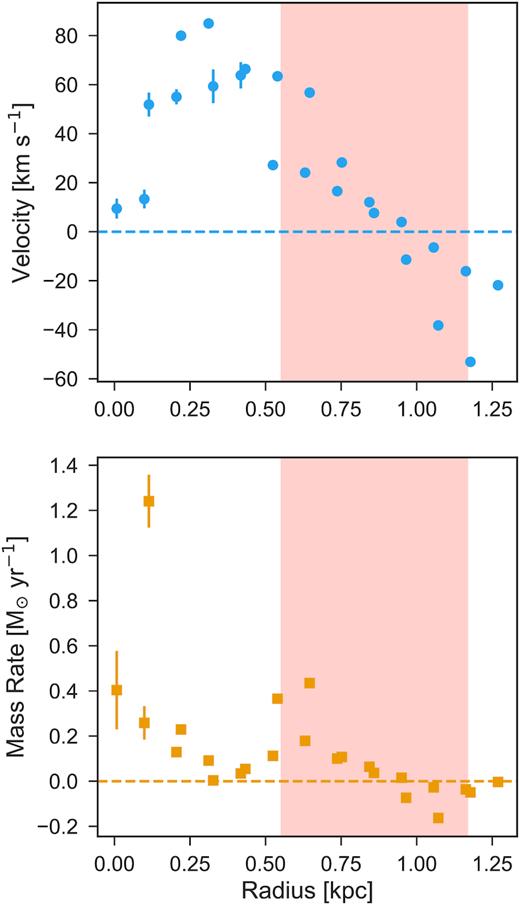
Radial profile of the residual flow velocity (blue) and flow mass (orange) calculated from concentric annuli placed on the residual velocity field of the molecular gas after removing the best-fitting rotating disc model (See Fig. 9). Negative values correspond to outflow while positive values correspond to inflow. The dashed lines indicate the transition from outflow to inflow for the velocity and mass rate. The red shaded region shows the radii where we observe the molecular gas ring. Inner to the ring we potentially observe outflow while outside the ring we observe inflow.

Open in new tabDownload slide

Fig. 10 also suggests radial inflow outside of 1kpc with velocities reaching 50 km s⁻¹. The mass inflow rate into the circumnuclear ring however is very small, only ∼0.1 M_|$\odot$| yr⁻¹. The strongest inflow residuals though do occur in the NW and SE edges of the ring, exactly where the dust lanes meet the ring and where we would expect to find signatures of inflowing gas.

3.3 The inner warped disc

Inside the ring, both the stars and gas dramatically change their distribution and kinematics. The bottom row of Fig. 5 shows a zoom in of the inner 6.5 arcsec for the F160W image and V−H dust map. We see inside from the contours of the continuum image and elongation along a P.A.∼ 85° shown as a white line. This was first observed by Shaw et al. (1993) who suggested the presence of a stellar nuclear bar possibly supported by the x₂ orbits of the main large scale bar. Wilson et al. (1993) however also suggested it could just be scattered nuclear light off dust from the AGN.

The dust map shows heavy extinction along an arc extending from the NE to SW directly across the nucleus. This is also the location of two strong concentrations of cold molecular gas that connect two sides of the ring. These two clumps straddle the very centre such that there is a lack of CO (2–1) emission at the location of the AGN and correspond to the double peaks seen in lower resolution CO (1–0) maps Petitpas & Wilson (2002). Perpendicular to the two clumps and the stream are also two distinct holes of CO (2–1) emission. These holes are aligned in the direction of the NLR and ionized gas outflow, and each have a radius of roughly 165 pc and cover a surface area of 8.6 × 10⁴ pc².

Using a 2 arcsec aperture and equation 2, we measure a molecular gas mass of ∼4 × 10⁷ M_|$\odot$|, or ∼25 per cent of the total molecular gas mass detected. Thus, while a large fraction of the molecular gas is contained within the rotating ring, a substantial amount seems to be experiencing irregular motion around the AGN.

The CO (2–1) line profiles near the centre contain multiple kinematic components which contribute to the increase of the measured velocity dispersion in the single Gaussian fits and are evidence for irregular motion. These kinematic components could be related to either the nuclear stellar bar or the ionized gas outflow so we performed a second fit of only the central 4 arcsec x 4 arcsec section of the ALMA cube. To fit each spaxel, we used the method described in Fischer et al. (2017) that employs the Bayesian MultiNest algorithm (Feroz, Hobson & Bridges 2009; Buchner et al. 2014) to fit emission line profiles and calculate the evidence for a particular fit. In this way, by comparing the evidence from a single component fit to a double component fit, we can determine whether the second component is statistically necessary. This can be extended up to any number of components, and in this work we allow for a maximum of three components based on visual inspection of the ALMA cube.

A complication after fitting for multiple kinematic components is associating each velocity component within each spaxel with the ones in the other spaxels to form a coherent picture of the gas kinematics. To accomplish this, we first determined the likely independent components that existed in the region by fitting the integrated CO (2–1) spectrum within the central 2 arcsec. We found five distinct kinematic components that have velocities of roughly −200, −100, 0, 100, and 200 km s⁻¹ which are shown together with the observed spectrum in Fig. 11. Then, for each of the components for a single spaxel fit, we associated it with one of the five components based on which one it was closest to in velocity. In this way, we constructed flux, velocity, and dispersion maps for each of the five components. Finally, based on inspection of each of the maps it was clear that the first and fifth components as well as the second and fourth components are the opposite sides of the same physical component so we plot them together. Fig. 12 shows the results of our fits and reconstruction of each molecular gas component where Comp1 refers to the original first and fifth components (±200 km s⁻¹), Comp2 refers to the original second and fourth components (±100 km s⁻¹), and Comp3 is the original third component (0 km s⁻¹).

Figure 11.

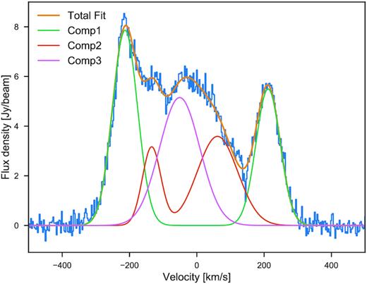
The integrated CO (2–1) spectrum within 2 arcsec of the nucleus (blue line) together with our fit using five kinematic components (orange line). We associate the two components with ±200 km s⁻¹ velocities (Comp1, green) and ±100 km s⁻¹ (Comp2, red) as single components. The final component near 0 km s⁻¹ is Comp3 (pink).

Open in new tabDownload slide

Figure 12.

Results of our multicomponent fitting in the inner 4 arcsec of the ALMA cube. Each spaxel was fit with up to three velocity components. Each of the best-fitting components were then grouped into five groups according to their velocity. The first and fifth components are plotted together in the top panel as Comp1. The second and fourth components are plotted together in the middle panels as Comp2. The third component is plotted in the bottom panels. The black contours plot the flux distribution of H₂ (1–0) S(1) from our SINFONI cube. In the middle panels, we also plot the kinematic major axis of the circumnuclear disc determined from our modelling of the larger scale CO (2–1) velocity field (purple), the ionized gas bicone region determined from the MUSE [O iii] flux map (gold), and the P.A. of the nuclear stellar bar shown also in Fig. 5 (green).

Open in new tabDownload slide

Our analysis therefore suggests the presence of three kinematically distinct cold molecular gas components in the nuclear region of NGC 5728. The first, shown in the top row of Fig. 12, is characterized by LOS velocities near 200 km s⁻¹ and a P.A.∼0°. The second, shown in the middle row, is characterized by LOS velocities around 100 km s⁻¹ and a P.A.∼45°, while the third component has LOS velocities near systemic and a kinematic P.A. that is unclear since the velocity gradient is weak but a flux P.A. near 90°.

We can also determine the mass of molecular gas that is contained within each kinematic component using again equation 2 and the conversions given above. We find a total mass within 2 arcsec for Comp1, Comp2, and Comp3 of 1.6 × 10⁷, 1.6 × 10⁷, and 7.7 × 10⁶ M_|$\odot$|, respectively. Thus about 40 per cent, 40 per cent, and 20 per cent of the total nuclear molecular gas is contained in Comp1, Comp2, and Comp3.

On all of the flux maps, we also plot the contours of H₂ (1–0) S(1)emission from the SINFONI cube. On the velocity maps, we plot the kinematic major axis for the circumnuclear rotating disc based on our fit in Section 3.2.3, the ionized gas bicone region based on the MUSE [O iii] map, and the major axis of the nuclear stellar bar based on Fig. 5.

Immediately it is clear that Comp1 likely corresponds to gas still in circular rotation in the inner part of the disc. However, it seems that as the molecular gas is rotating towards the bicone, the gas is being accelerated giving rise to the enhanced velocities seen here and in the residuals of the disc modelling (see Fig. 9). However, as soon as the gas rotates into the bicone, all CO (2–1) emission disappears given none of the components we identified show any correspondence with the bicone. We discuss possible reasons for the disappearance of CO (2–1) emission in Section 3.7.

Comp2, however, seems to be aligned perpendicular to the bicone at least within the central 1 arcsec. Based on our later modelling of the ionized gas, we find an inclination for the bicone of 49°compared to an inclination for the disc of 43°. Since the bicone is directed almost straight into the disc, the molecular gas must warp by 90° in the inner nuclear region. Based on the P.A. shift for Comp2 compared to the larger scale disc and Comp1, we associate Comp2 with a warped inner rotating molecular disc that is contributing to shaping the bicone and likely providing the material necessary to fuel the AGN. Comp2 is further directly associated with the strong extinction seen in Fig. 5 and is therefore also providing the obscuration necessary to hide the BLR. It also has a relatively high-velocity dispersion of ∼80 km s⁻¹ also indicating a thick disc which are commonly found in the central few 100 pc of AGNs (Hicks et al. 2009; Riffel & Storchi-Bergmann 2011a; Alonso-Herrero et al. 2018).

Comp3 perhaps is related to gas streaming along the nuclear bar. The velocities near 0 km s⁻¹ therefore are due to the orientation of the bar in the plane of the sky. Petitpas & Wilson (2002) were searching exactly for this molecular gas aligned with the nuclear stellar bar but were unable to detect it likely due to the low spatial resolution of their data. The thought was that nuclear gas in the bar would be an indication that the nuclear stellar bar would be driving gas further inward towards the AGN. However, we see here that while it does seem that there is molecular gas associated with the nuclear bar, the primary component that is driving gas to the centre is instead Comp2 which itself is arranged in a bar-like structure. This nuclear molecular gas bar then is significantly leading the stellar bar and in fact could be related to the x₂ orbits of the nuclear stellar bar which are perpendicular to the major axis of a bar. Hydrodynamical simulations do indicate that gaseous bars should lead stellar bars when both exist (Friedli & Martinet 1993; Shaw et al. 1993) however note these simulations primarily consist of a single stellar and gaseous bar whereas for NGC 5728 we are observing a secondary nuclear and gaseous bar. The three molecular gas components make for a seemingly chaotic environment around the AGN and is likely not a dynamically stable set-up without collisions between gas clouds. It is possible though that this contributes to the variability of AGNs where short-lived, unstable molecular gas environments quickly feed the AGN before breaking itself apart with the help of AGN feedback.

The morphology of H₂ (1–0) S(1) emission seems to be a combination of all three components. The distinct S-shaped structure looks to follow the edges of Comp1 while the slight extension in the middle from NE to SW is either related to Comp2 or Comp3. The biggest difference between H₂ (1–0) S(1) and CO (2–1) is that the peak of H₂ (1–0) S(1)is directly located on the position of the AGN while the peaks of CO (2–1) straddle the centre. This combined with extended morphology following the edges of CO (2–1) emission suggests that the H₂ (1–0) S(1) emission is produced by either X-ray heating from the AGN or shocks as the AGN driven outflow expands into the disc and is consistent with the conclusions of a study of NIR line emission in 62 AGN from long slit spectra (Rodríguez-Ardila et al. 2004; Rodríguez-Ardila, Riffel & Pastoriza 2005; Riffel et al. 2013b). Indeed Durré & Mould (2018) show that this is the case through the use of H₂ excitation diagrams.

3.4 AGN driven outflow

3.4.1 NLR morphology

From the MUSE [O iii] maps (Fig. 3) we find the NLR in a biconical shape that seems to be ‘piercing’ through the centre of the ring and has an apex exactly at the location of the AGN. Particularly noticeable is the strong dip in [O iii] emission towards the NW that indicates obscuration by the nuclear star-forming disc. Combined with the fact that the SE emission is systematically brighter than the NW emission, the NLR is inclined such that the bicone is in front of the nuclear disc towards the SE and behind the disc towards the NW until it breaks through at larger radii. This interpretation is consistent with previous studies of NGC 5728 using HST narrow band imaging (Wilson et al. 1993) and lower spatial resolution IFU observations (Davies et al. 2016).

We measure a biconical NLR extent of 1.7 kpc to the SE and 2.1 kpc to the NW. The central PA is roughly −60° and the full opening angle is ∼55°. The NLR emission, while extended out to kpc scales, is largely concentrated in two clumps on opposite side of the AGN. The brightest clump in the SE is only 130 pc away from the AGN while the NW one is about 230 pc. Separating the two clumps is another gap in emission that spatially corresponds to the Comp2 component of the cold molecular gas shown in Fig. 12 and suggests that it is the component that is obscuring the AGN and producing the biconical shape of the NLR. The reason that the gap in [O iii] emission does not fully align with the Comp2 molecular gas component is due to the inclination of the bicone. The SE side of the bicone is in front of Comp2 while the NW side is behind it such that the gap in [O iii] emission appears to the NW of the location of Comp2. What is abundantly clear though is that the cavities of cold molecular gas are filled with warm ionized gas.

On smaller scales from the SINFONI data (Fig. A3), we find that the ionized emission is largely confined to the NLR showing again a biconical structure and extending from the SE to the NW, similar to the [O iii] emission from MUSE. The brightest emission for all three emission lines ([Fe ii], [Si vi], and Br γ) is concentrated towards the SE, and with the higher spatial resolution of SINFONI, we locate it only 20 pc away from the AGN. Interestingly, [Fe  ii] shows the same ‘hook’ structure to the NW as the H₂ (1–0) S(1) emission, except at locations inward from H₂ (1–0) S(1). Both [Si vi] and Brγ instead are distributed in distinct clouds and have an overall shorter extent compared to [Fe ii] and H₂ (1–0) S(1). Fig. 13 highlights the spatial differences between the different phases of the gas with warm molecular gas (red) encompassing the partially ionized gas (green; [Fe ii]) which then encompasses the fully ionized gas (blue; [Si vi]). This observed ‘stratification’ of the ionization structure of the gas around the nucleus strongly suggests that the AGN is the source of the ionization. This is also further evidence that the so-called ‘Coronal Line Region’ is simply the inner part of the NLR where the ionizing radiation field is stronger and can produce lines with higher ionization potential.

Figure 13.

Three colour image of the central 4 arcsec x 4 arcsec of NGC 5728 from SINFONI. Red, green, and blue colours indicate emission from H₂ (1–0) S(1), [Fe  ii], and [Si vi], respectively. The black cross marks the location of the AGN.

Open in new tabDownload slide

3.4.2 Ionized gas kinematics

In the nucleus, and spatially corresponding to the brightest clumps of ionized gas emission, we find elevated velocities reaching  +/−400 km s⁻¹. The kinematic P.A. is along the same direction as the NLR and we see larger dispersions, although some of them are due to beam smearing and the presence of multiple kinematic components as in the cold molecular gas. All of this evidence points towards the presence of an AGN driven outflow, and the high spatial resolution SINFONI observations only further increase support for this interpretation. All of the SINFONI detected ionized emission lines show high velocities along the major axis of the NLR and dispersions reaching over 300 km s⁻¹ (see Fig. A3). In particular, the [Si vi] line displays the largest velocities reaching 500 km s⁻¹. Both Br γ and [Fe  ii] show in general the same velocity structure albeit with slightly lower absolute velocities. This is in contrast to the H₂ (1–0) S(1)kinematics which show much lower velocities and dispersions and suggests there is a lack of molecular gas in the outflow due to the AGN inflating a bubble in the disc such as the one seen in NGC 1068 (May & Steiner 2017).

3.4.3 Outflow modeling

Building on the outflow interpretation of the ionized gas kinematics, we used dysmalpy to model and fit for the outflow parameters. As we did for modelling the rotating disc, we used the 2D velocity map as our input and specifically decided on the [Si vi] velocity map since it shows the strongest outflow signatures. Our biconical outflow model is similar to those that have been extensively used in the literature for modelling the kinematics of gas around nearby AGNs based on both long slit data (e.g. Crenshaw & Kraemer 2000; Crenshaw et al. 2000, 2010; Das et al. 2005, 2006; Fischer et al. 2013, 2014) as well as IFU data (e.g. Müller-Sánchez et al. 2011; Bae et al. 2017). The model consists of two axisymmetric cones that share an apex at the location of the AGN. The cones have two opening angles, an inner (θ_inner) and outer (θ_outer) opening angle that define the walls of the cone and where the emission originates. The bicone also has an inclination (i_bicone where 0° indicates the cones are oriented along the line of sight) and position angle (P.A._bicone) on the sky with respect to the line of sight.

As in Bae & Woo (2016), we assume the flux is exponentially decreasing with radius according to |$F(r) = A\mathrm{ e}^{-\tau r/r_{\mathrm{ end}}}$| where r_end is the radial edge of the bicone and τ controls the speed at which the flux falls off. Given we are only fitting the velocity map, we fixed τ to be 5 which is the value found for many nearby AGN. Finally, the model allows for different velocity profiles that change as a function of radius. We chose a linearly increasing profile that reaches a maximum (v_max) at a specific radius (r_turn) then decreases linearly until r_end. This assumes a radially symmetric profile such that r_end = 2r_turn. As with modelling the rotating disc, we determined the best-fitting parameters using MCMC with 800 walkers, 100 burn steps, and 100 sampling steps.

Fig. 14 shows the results of our outflow fitting. We find best-fitting outflow parameters of θ_inner = 18 ± 1°, θ_outer = 23 ± 1°i_bicone = 49 ± 2°, P.A._bicone = 43 ± 2°, r_end = 540 ± 20 pc, and v_max = 737 ± 25 km s⁻¹ based on the median and standard deviations of the resulting posterior distributions.

Figure 14.

Results of fitting the [Si vi] velocity field with a biconical outflow model. The observed velocity field is shown in the left-hand panel, the best-fitting model in the middle panel, and the residuals in the right-hand panel.

Open in new tabDownload slide

Comparing the spatial orientations of the disc and outflow, we see that our initial interpretation that the NLR is in front of the disc towards the SE and behind the disc towards the NW is correct. The disc is inclined at an angle of 43° with respect to the LOS, while the outflow is inclined by 49°. However, an outer half opening angle of 23° places the front side of the NLR at only an angle of 26°, well in front of the disc. The similarity of the inclinations for both the disc and the outflow further shows that the NLR is completely intersecting the disc. The turnover radius for the outflow is only 270 pc which explains why we only observe enhanced velocities very near to the centre in the MUSE maps. Thus, while the NLR extends out to 2 kpc only the very central regions are outflowing and the rest is simply AGN excited gas within the disc.

3.5 Outflow energetics

In this section, we explore the ionized gas energetics within the outflow. Because of the short extent of the outflow, we primarily use the diagnostics available from the SINFONI cube to spatially resolve the outflow properties. In particular, we want to measure the mass outflow rate, mechanical energy rate, and momentum rate as a function of radius and compare to the energy and momentum injection from the central AGN.

Similar to our analysis of the electron density radial profile in Appendix  B, we binned the SINFONI cube using annular apertures along the SE redshifted half of the NLR given extinction is not as much of a factor. For the SINFONI data, we chose an annular width of 0.075 arcsec which is half the PSF size and extended out to 1.65 arcsec. Within each aperture, we fit the [Si vi] and Br γ line profile with either 1 or 2 Gaussian components, choosing between them based on log (evidence) as we did for the very central regions of the ALMA data. If the profile needed two components, we calculated a flux-weighted average velocity since we assume that all of the emission in the inner regions is related to the outflow.

The upper panel of Fig. 15 plots the resulting velocity profile for both [Si vi] and Br γ with all radii and velocities deprojected based on the inclination from the best-fitting 2D model from Section 3.4.3. Both ionized gas lines show essentially the same profile, implying that both lines are tracing the same physical components of gas. The narrow and broad components are also both increasing with radius up to ∼250 pc, then decreasing towards larger radii just as we modelled previously. The general consistency of both the narrow and broad component suggests that these are also tracing the same gas and merely reflect the underlying velocity distribution of the gas. We also show the few inner bins of the [O iii] velocity profile from MUSE which traces roughly the same shape except a bit more flattened due to the larger beam size of the MUSE observation. We further show the velocity profiles from the stars and the best-fitting rotating disc model used to fit the CO (2–1) velocity map. These both show a nearly flat profile around 0 km s⁻¹ since the bicone axis is aligned nearly along the minor axis of the disc.

Figure 15.

Radial profiles of the outflow velocity (top panel), mass outflow rate (second panel), outflow kinetic luminosity (third panel), and momentum rate (bottom panel) determined from concentric annuli spanning the redshifted side of the NLR. Velocity profiles are shown for [Si vi], Br γ, [O iii], the stars, and CO (2–1). The CO (2–1) velocities were inferred from the best-fitting rotating disc model due to the lack of CO (2–1) emission in the bicone. The dashed vertical line indicates the best-fitting turnover radius from our 2D outflow modelling of the [Si vi] velocity map.

Open in new tabDownload slide

The peak mechanical energy in the outflow is well below the AGN luminosity, L_Bol = 1.4 × 10⁴⁴ erg s⁻¹, only reaching 0.003 per cent of L_Bol. Similarly, the ratio of the momentum rate to the radiation momentum rate from the AGN (L_Bol/c) is only 0.043. These properties all suggest that the outflow currently is not energy driven but rather momentum driven given their extremely low values (e.g. Faucher-Giguère & Quataert 2012; Zubovas & King 2012).

While the values seem quite low, we can compare them to the properties of outflows found across literature. Fiore et al. (2017) recently compiled a comprehensive set of outflow energetics from various studies over the years spanning a large range of AGN luminosity. They used this data to establish clear AGN wind scaling relations, in particular between the mass outflow rate and outflow power with the AGN bolometric luminosity in all phases of the gas in the outflow.

In Fig. 16, we compare our values of |$\dot{M}_{\rm {out}}$| and |$\dot{E}_{\rm {out}}$| for NGC 5728 with the ionized wind data from Fiore et al. (2017). NGC 5728 lies very close to the correlations and the low values of |$\dot{M}_{\rm {out}}$| and |$\dot{E}_{\rm {out}}$| seem to be simply due to the relatively modest AGN luminosity. With only one point, we cannot definitively determine if the correlations presented in Fiore et al. (2017) actually extend to lower luminosities. Therefore, we compiled more values for |$\dot{M}_{\rm {out}}$| and |$\dot{E}_{\rm {out}}$| with a focus on AGN with |$L_{\rm Bol} \lesssim 10^{46}$| erg s⁻¹. We found data for 15 AGN: NGC 1068, NGC 2992, NGC 3783, NGC 6814, NGC 7469 (Müller-Sánchez et al. 2011), NGC 4151 (Crenshaw et al. 2015), Mrk 573 (Revalski et al. 2018a), Mrk 34 (Revalski et al. 2018b), NGC 7582 (Riffel et al. 2009a), Mrk 1066 (Riffel & Storchi-Bergmann 2011a), Mrk 1157 (Riffel & Storchi-Bergmann 2011b), Mrk 79 (Riffel, Storchi-Bergmann & Winge 2013a), NGC 5929 (Riffel, Storchi-Bergmann & Riffel 2015), NGC 2110 (Schnorr-Müller et al. 2014), and NGC 3081 (Schnorr-Müller et al. 2016). Finally, we also include the sample of 234 type 2 AGN studied in BN19 using single integrated SDSS spectra and dust SED fitting.

Figure 16.

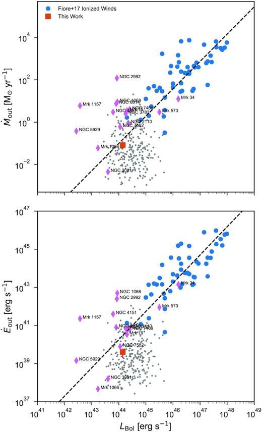
Correlations between the mass outflow rate (⁠|$\dot{M}_{\rm {out}}$|⁠; top panel) and kinetic outflow power (⁠|$\dot{E}_{\rm {out}}$|⁠; bottom panel). Blue points are the data compiled by Fiore et al. (2017) and the orange square plots our values for NGC 5728. Purple diamonds are compiled from various literature sources for more modest AGN luminosities. See the text for the specific references for each of the AGN. Grey points are the type 2 AGN studied in Baron & Netzer (2019). The black dashed lines show the best-fitting correlations from Fiore et al. (2017).

Open in new tabDownload slide

The inclusion of both single source literature compilation and the BN19 sample shows that while NGC 5728 lies close to the Fiore et al. (2017) correlations, there is likely substantial scatter at lower luminosities. That said, combining all of these samples together can be dangerous given the widely varying methods and data quality used to measure these properties. In particular, while Fiore et al. (2017) renormalized all outflow properties to a constant electron density, BN19 showed that object by object determined densities can change the mass outflow rate considerably and thus weaken the mass outflow rate correlation. What is needed to confirm these correlations is a large, spatially resolved sample of AGN where all of these properties can be properly and systematically measured.

3.6 AGN feedback in NGC 5728

With such a low mass outflow rate and outflow power, it is unlikely that the AGN driven wind is effectively suppressing star formation in NGC 5728 and affecting its evolution. With a total molecular gas mass in the circumnuclear disc of 10^8.1 M_|$\odot$|, it would take 217 Myr to completely clear the disc of its gas even including the potential molecular gas outflow. Using Herschel photometry and SED fitting, Shimizu et al. (2017) estimated a global SFR of 2.1 M_|$\odot$| yr⁻¹. Combining this with |$\dot{M}_{\rm {out}}$|⁠, the total gas depletion time still 47 Myr. However, this is under the assumption that all of the outflowing gas can escape the gravitational potential of the galaxy. Following Rupke, Veilleux & Sanders (2002), we can estimate the escape velocity under the assumption of a truncated isothermal sphere, |$v_{\rm esc}(r) = \sqrt{(}2)v_{\rm circ}[1 + \ln (r_{\rm max}/r)]^{1/2}$|⁠. We assume an r_max = 100 kpc and use v_circ = 320 km s⁻¹ from Rubin (1980). At 250 pc, the radius of peak outflow velocity, v_esc = 1200 km s⁻¹, far above the outflow velocities of either the ionized or molecular gas. Outflows in moderate luminosity AGNs do not seem to have the energy to escape their host galaxies as this has been observed in many other systems (e.g. Davies et al. 2014; Fischer et al. 2017; Herrera-Camus et al. 2019).

We can further compare the mass outflow rate with the mass flow rate through the bicone. Using the best-fitting parameters for the outflow, the total surface area covered by the bicone is 0.19 kpc². From our disc modelling we find an average rotational velocity of the molecular gas of 273 km s⁻¹ through the bicone. Combined with the average surface mass density of 55 M_|$\odot$| pc⁻², we calculate that molecular gas flows through the bicone at a rate of ∼9.5 M_|$\odot$| yr⁻¹, about 16x higher than the mass outflow rate. Essentially, the gas that is entering the bicone is not being ejected at rates large enough that would substantially disturb the structure and dynamics of the disc. This is especially true when we take into account the fact that the molecular gas is only moving radially at speeds of 40 km s⁻¹ which means that by the time it exits the bicone it has only moved about 55 pc.

3.7 Missing molecular gas?

The most striking evidence of AGN feedback is the presence of what appears to be large ‘holes’ of cold molecular gas as probed by CO (2–1) emission that are co-located exactly along the outflow and NLR. Therefore, it’s reasonable to interpret that the AGN driven outflow has completely evacuated these regions of the disc of molecular gas. However, these holes do not exist in maps of the ionized gas and in fact it is these regions where emission from ionized gas is strongest. If an AGN driven outflow had indeed evacuated these regions, we should expect it to drive out all phases of gas.

A plausible explanation for these holes is instead that CO (2–1) is not accurately tracing the presence molecular gas in the NLR. Under standard ISM conditions, CO (2–1) would be a reliable tracer of the molecular gas mass, however in the presence of the strong radiation field of an AGN, it could be that the CO (2–1) line in particular or all CO lines are suppressed. Whereas in a normal star-forming disc, molecular gas is primarily heated by nearby OB stars with FUV photons dominating the process, near an AGN, X-rays will dominate over FUV photons and control the heating and chemical composition of the gas producing a so-called X-ray dissociation region (XDR).

This is being increasingly observed in local AGNs. Both Rosario et al. (2019) and Feruglio et al. (2019) reported recently on a lack of CO (2–1) emission near the central AGN that is instead filled with H₂ (1–0) S(1) and ionized gas emission. These cavities of CO emission are further cospatial with hard X-ray emission, confirming that X-ray radiation is suppressing the CO emission. While we observe the same effect at the very centre of the galaxy corresponding to the location of the AGN, we do not observe H₂ (1–0) S(1) emission filling the larger scale CO (2–1) holes that correspond to the bicone. Instead, H₂ (1–0) S(1) is only lining the edges of the bicone where gas is entering the bicone. It is possible then that the inner NLR is devoid of molecular gas and a continuation of the stratification we observe in the SINFONI line emission continues on larger scales, i.e. that cold molecular gas only exists outside the bicone region with hotter and hotter gas becoming more prevalent towards the inner NLR. To confirm the lack of molecular gas in the NLR, however, observations of higher-J CO lines are needed.

4 SUMMARY AND CONCLUSIONS

We have presented a comprehensive analysis of multiwavelength data sets for the nearby Seyfert 2 galaxy, NGC 5728. Using primarily HST imaging and MUSE, SINFONI, and ALMA cubes, we measured and analysed the distribution and kinematics of the stars, ionized gas, and molecular gas. Our results and conclusions are summarized as follows:

• Prominent dust lanes are observed extending along the major axis of the large stellar bar from the outer disc to the circumnuclear ring. These are likely coincident with the primary shocks produced by the axisymmetric bar potential and driving inflow to the circumnuclear region.

• The circumnuclear ring is observed as a ring of low stellar velocity dispersion, bright H α clumps, and CO (2–1) emission indicating the presence of on ongoing star formation and young stars. This star formation is likely induced by the build-up of gas at the ILR of the primary bar. The kinematics of the ring are well fit by circular rotation, however we also seen signs of inflow into the ring where the ring and dust lanes meet at a rate of 1 M_|$\odot$| yr⁻¹.

• Inside the ring, we find a three distinct kinematic components of the molecular gas corresponding to gas rotating with the ring, gas inflowing to the AGN, and gas following the nuclear stellar bar. The gas inflowing to the AGN is distributed across the nucleus at the location of heavy extinction and is the source of obscuration for the AGN due to its perpendicular orientation compared to the NLR.

• The AGN is driving a weak outflow primarily seen in ionized gas with a mass outflow rate of 0.08 M_|$\odot$| yr⁻¹ that only reaches to radii of 250 pc before decelerating down to stellar rotation velocities. There are hints of molecular outflow in residuals of the disc modelling indicating a molecular mass outflow rate of 1 M_|$\odot$| yr⁻¹ but only 40 km s⁻¹velocity. We determine that the outflow is unlikely to be largely disturbing the structure of the circumnuclear disc.

• We observe cavities of CO emission co-spatial with the AGN outflow that could either be explained by a deficiency of molecular gas in the NLR or a suppression of CO emission by the hard X-ray radiation of the AGN.

Overall, for NGC 5728, we find signatures of both feeding and feedback of the AGN. However, feeding of both the AGN and central region of the galaxy is currently the dominant process. NGC 5728 would need a large increase to its accretion rate to boost the energetics of its outflow and severely disrupt its evolution.

ACKNOWLEDGEMENTS

We thank the anonymous referee for helpful comments and suggestions that improved the paper. We thank Cheng-Yu Kuo from the Megamaser Cosmology Project for sharing the coordinates of the AGN in NGC 5728. TTS thanks Travis Fischer for sharing and discussing his line decomposition software package as well as discussing the results of this paper. This paper makes use of the following ALMA data: ADS/JAO.ALMA#2015.1.00086.S. ALMA is a partnership of ESO (representing its member states), NSF (USA) and NINS (Japan), together with NRC (Canada) and NSC and ASIAA (Taiwan) and KASI (Republic of Korea), in cooperation with the Republic of Chile. The Joint ALMA Observatory is operated by ESO, AUI/NRAO and NAOJ. This research has made use of the NASA/IPAC Extragalactic Database (NED), which is operated by the Jet Propulsion Laboratory, California Institute of Technology, under contract with the National Aeronautics and Space Administration. This research has made use of NASA’s Astrophysics Data System Bibliographic Services. This research made use of astropy,⁵ a community-developed core python package for Astronomy (Astropy Collaboration 2013, 2018).

Footnotes

REFERENCES

APPENDIX A: FULL FOV EMISSION LINE FITS

Figure A1.

Single Gaussian fits to the H α, [N ii], and [O iii] lines detected in the MUSE cube. Left column shows the integrated flux normalized to the maximum flux, middle column shows the velocity, and the right column shows the velocity dispersion. Velocity dispersions have been corrected for instrumental line broadening. In all frames, North is up and East is to the left. The black cross locates the position of the AGN.

Open in new tabDownload slide

Figure A2.

Same as Fig. A1 for H β, [S ii], and [O i]. The [S ii] flux map indicates the combined flux of the λ6716 and λ6731 lines.

Open in new tabDownload slide

Figure A3.

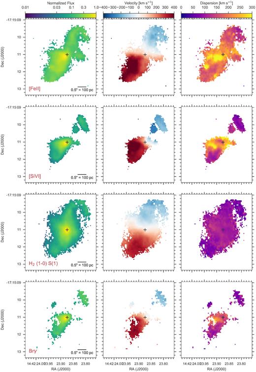
Single Gaussian fits to the prominent emission lines detected in the H + K band SINFONI cube. Left column shows the integrated flux normalized to the maximum flux, middle column shows the velocity, and the right column shows the velocity dispersion. Velocity dispersions have been corrected for instrumental line broadening. In all frames, North is up and East is to the left. The black cross locates the position of the AGN.

Open in new tabDownload slide

Figure A4.

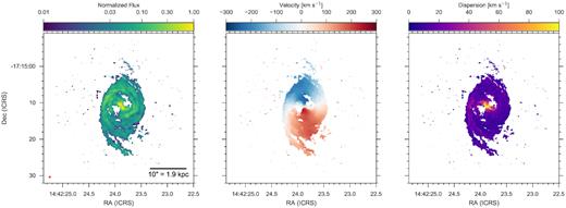
Results of a single Gaussian fit to the ALMA CO 2–1 data. Left, middle, and right columns show the normalized integrated flux, velocity, and velocity dispersion. The small red ellipse in the bottom right corner indicates the size of the beam.

Open in new tabDownload slide

APPENDIX B: ELECTRON DENSITIES

An important diagnostic IFU studies can provide is the electron density (n_e) of the ionized gas. The electron density is needed in particular for the determination of mass outflow rates for both star formation and AGN driven outflows. Historically, these have been measured from single spectra using the [S ii]λλ6716,6731 line ratio with high uncertainties or assumed based on local studies with usual estimates of |$n_{\rm e}\lt 100\, \rm {cm}^{-3}$|⁠. Recently, IFU studies have begun to spatially resolve the electron density distribution within individual galaxies at low redshift (e.g. Kakkad et al. 2018; Nascimento et al. 2019). At high redshift, stacks of the nuclear spectra from IFU surveys have produced estimates of the electron density for both H ii regions and broad outflows (Förster Schreiber et al. 2019). These studies have all indicated that the assumed electron densities have been underestimated which in turn can greatly overestimate the mass outflow rate.

We use three independent methods to determine the electron density in the circumnuclear region of NGC 5728. The first and most popular method in the literature uses the [S ii] doublet ratio as the density diagnostic due to the weak dependence on electron temperature. With a critical density around 1000 cm⁻³ the [S ii] line ratio provides reliable electron densities within the range of 50–2000 cm⁻³. Above or below these densities however, the [S  ii] doublet ratio saturates and becomes unresponsive to higher or lower densities.

The second method, introduced by Holt et al. (2011) and used extensively in Rose et al. (2018) and Santoro et al. (2018), incorporates the ratios of four auroral or trans-auroral emission lines: the [O ii] doublets λλ3726,3729 and λλ7319,7330 and the [S ii] doublets λλ4069,4076 and λλ6716,6731. This method constructs line ratios from the total flux between the doublets instead of the flux in individual lines and is therefore less susceptible to degeneracies in decomposing the doublets. The large wavelength range further provides an estimate of the gas reddening. As shown by Holt et al. (2011), this diagnostic is also sensitive to a much larger range of electron densities than the single [S ii]λλ6716,6731 line ratio (10²–10^6.5 cm⁻³). However, both [O ii] doublets and the [S ii]λλ4069, 4076 doublet are usually weak and to simultaneously measure all four doublets requires either multiple spectra or a spectrum that covers a large wavelength range.

The third method was developed in Baron & Netzer (2019, hereafter BN19) and we provide a brief summary here. Instead of using the weak auroral and trans-auroral lines, they calibrated a method of measuring n_e using the strong [O iii], H α, H β, and [N ii] lines under the assumption that the gas is photoionized by an AGN. They found that the [O iii]/H β and [N ii]/H α line ratios can provide a reliable measure of the ionization parameter following a simple equation which can then be converted into an electron density assuming the radial distance to the AGN is known.

MUSE does not extend to short enough wavelengths for the trans-auroral analysis, but as part of the LLAMA programme, we obtained X-Shooter IFU spectra for all of the targets. For NGC 5728, we detected all four of the auroral or trans-auroral doublets in the spectrum extracted from a central 1.8 arcsec box aperture. In Fig. B1, we show cut-outs of the X-Shooter spectrum around the four doublets. Unfortunately the [O ii]λλ3726,3729 doublet is next to the edge of one of the UVB echelle orders which caused the increased noise blue-ward of the doublet.

Figure B1.

X-Shooter spectrum cut-outs (purple) around the four trans-auroral doublets [S ii]λλ6716,6731 (top left); [S ii]λλ4069,4076 (top right); [O ii]λλ3726,3729 (bottom left); and [O ii]λλ7319,7330 (bottom right). Overplotted are the best-fitting model (orange) and its red-shifted (red, dashed), blue-shifted (blue, dashed), and systemic (green, dashed) components. Spectra have been normalized to the maximum value of the cutout and the x-axis converted to velocities relative to the blue component of the doublet.

Open in new tabDownload slide

To determine the necessary kinematic components to model the doublets, we first fit the [O iii]λλ4959,5007 emission lines to use as a robust template for the presence, location, and width of the existing kinematic components comprising the ionized gas as we recently did for this same galaxy in Shimizu et al. (2018). In fitting the [O iii] doublet, we fixed the velocity and dispersion of the components to be the same between each of the lines and fixed the intensity ratio (5007/4959) to 3, the theoretical value. The aperture used to produce the X-Shooter spectrum encompasses both sides of the outflow so we used a combination of red and blue-shifted Gaussian components in our model. To properly reproduce the [O iii] line profile, we found we needed six kinematic components, three red-shifted, and three blue-shifted.

In fitting the auroral and trans-auroral lines, we fixed the velocity and dispersions of all of these components but left the intensities to vary. However, we found while fitting the [S ii]λλ6716,6731 doublet that we needed to include a seventh component with 0 km s⁻¹ velocity and 168 ± 7 km s⁻¹ dispersion. The remaining three doublets were then well fitted with these seven components. Fig. B1 shows the best-fitting model for each of the doublets as well as the combined red-shifted, blue-shifted, and systemic components of the model.

While the fits overall are satisfactory, the low S/N and relatively small separation of three of the doublets creates strong degeneracies between the amplitudes of the individual components. However, as mentioned previously, the electron density measurement from the trans-auroral lines is only dependent on the total flux of each of the doublets. Therefore, for NGC 5728 the combined auroral and trans-auroral lines can provide a robust estimate of the flux-weighted electron density but cannot provide separate electron densities for each of the kinematic components.

Fig. B2 plots the location of the [S ii] and [O ii] doublet ratios along with the expected values for a grid of models with different E(B − V) and n_e. The models are the same as those presented in Rose et al. (2018) and were produced using the cloudy photoionization code under the assumptions of solar metallicity gas photoionized by a central source with a power law continuum (α = −1.5 for F_ν ∝ ν^α). They varied the electron density of the gas to model intrinsic trans-auroral line ratios and then applied a Calzetti et al. (2000) reddening law for a range of E(B − V).

Figure B2.

Trans-auroral line ratio diagram showing the location of the [S ii](4069 + 4076/6716 + 6731) and [O ii](3726 + 3729/7319 + 7330) ratios for NGC 5728 (purple point). The black lines with points plot the values generated from a grid of cloudy models with a range of log n_e and E(B − V).

Open in new tabDownload slide

Using 2D spline interpolation, we estimated the best-fitting |$\log \, n_{\rm e}$| and E(B − V) for NGC 5728 assuming they vary smoothly as a function of the trans-auroral line ratios. Taking into account only the uncertainties on the line ratios, we estimate a flux-weighted log n_e = 3.19 ± 0.12 (1550 cm⁻³) and E(B − V) = 0.18 ± 0.05.

Within the same X-Shooter spectrum, we then fit the H α + [N ii] complex and H β line profile using the same kinematic components to determine n_e via the BN19 method. As a comparison to the trans-auroral estimate, we only calculated [O iii]/H β and [N ii]/H α line ratios for the total line profile. From the line ratios, we measure a log U = −2.59 ± 0.11. The biggest uncertainty here is what radial position to choose to convert log U into an electron density. We chose 171 pc which corresponds to half the size of the X-Shooter aperture. We find log n_e = 3.20 which agrees well with the value from the auroral and trans-auroral lines.

We can compare this to using only the [S ii]λλ6716,6731 line ratio. We find an [S  ii] 6716/6731 ratio of 0.65 ± 0.34. Using the pyneb⁶ software package and assuming an electron temperature of 10⁴ K, this translates to a log n_e = 3.36 ± 0.95 (2300 cm⁻³). Clearly the large amount of blending between the [S ii] doublet lines causes severe degeneracies and leads to almost a factor of ten uncertainty even though the value agrees quite well with the trans-auroral value.

We also compared the X-Shooter derived n_e with ones obtained from the MUSE cube based on both the [S ii] 6716/6731 ratio and the BN19 method. We measured the line fluxes using annular slices along a PA of −65° West of North, i.e. along the bicone axis. The annular slices spanned angles  +/−20° away from the centre, had a width of 0.5 arcsec, and ranged from 0 to 11.5 arcsec away from the AGN. We chose to only use the redshifted SE side of the NLR since it is most unaffected by extinction and has higher S/N. Fig. B3 plots the annular apertures on top of the [O iii]λ5007 flux map from our single Gaussian fits to the MUSE cube and shows how the annuli cover the majority of the biconical structure of the NLR.

Figure B3.

[O iii]λ5007 flux map of the central 12 arcsec from the MUSE cube. Overlaid are the locations of the annular apertures used to measure the properties of the NLR. The black cross shows the location of the AGN.

Open in new tabDownload slide

Spectra were extracted from each of the apertures and the [O iii] doublet was again fit first to determine the necessary number of kinematic components in the model since the spatial location, aperture size, spectral resolution, and S/N is different from the X-Shooter spectrum. The H β, H α + [N ii] complex, and [S ii] doublet were then fit with the same components.

Fig. B4 plots n_e as a function of radius as determined by the [S ii] 6716/6731 ratio and the BN19 method from the MUSE cube. Also plotted in the centre is our estimate from the X-Shooter spectrum. Inside of 1kpc, there is a strong increase of n_e based on BN19, whereas the [S ii] based n_e slightly decreases toward the centre. This is due to the strong blending of the [S ii] 6716/6731 doublet in the centre where the velocity gradient is large and there are multiple kinematic components. Therefore a robust [S ii] doublet measurement of the electron density becomes very difficult without high spectral resolution. The BN19 based values are also very well aligned with the auroral and trans-auroral based value which is the most robust estimate. It is clear then that within 1 kpc, n_e ≈ 1000 cm⁻³, therefore for all later analysis we will use the auroral and trans-auroral value as the electron density of the gas. At larger radii, we note there is better consistency between the BN19 and [S ii] doublet methods but still some discrepancies which could be explained by the different emission regions for the various lines. It is possible that while [O iii] and H α are being emitted throughout a whole ionized cloud, [S ii] instead is only emitted at the ionization front.

Figure B4.

Radial profile of |$\log \, n_{\mathrm{ e}}$| along the redshifted side of the NLR axis and within apertures shown in Fig. B3. The blue solid points plot the measurement using Gaussian fitting of the [S ii] doublet emission line profile while the green squares plot the measurement based on optical line ratios and the method from Baron & Netzer (2019). The orange point shows the n_e measurement from our trans-auroral emission line analysis and the open red square shows the BN19 measurement from the X-Shooter optical line ratios.

Open in new tabDownload slide