


ABSTRACT
We study the polarization properties of extragalactic sources at 95 and 150 GHz in the SPTpol 500 deg2 survey. We estimate the polarized power by stacking maps at known source positions, and correct for noise bias by subtracting the mean polarized power at random positions in the maps. We show that the method is unbiased using a set of simulated maps with similar noise properties to the real SPTpol maps. We find a flux-weighted mean-squared polarization fraction 〈p2〉 = [8.9 ± 1.1] × 10−4 at 95 GHz and [6.9 ± 1.1] × 10−4 at 150 GHz for the full sample. This is consistent with the values obtained for a subsample of active galactic nuclei. For dusty sources, we find 95 per cent upper limits of 〈p2〉95 < 16.9 × 10⁻³ and 〈p2〉150 < 2.6 × 10⁻³. We find no evidence that the polarization fraction depends on the source flux or observing frequency. The 1σ upper limit on measured mean-squared polarization fraction at 150 GHz implies that extragalactic foregrounds will be subdominant to the CMB E and B mode polarization power spectra out to at least ℓ ≲ 5700 (ℓ ≲ 4700) and ℓ ≲ 5300 (ℓ ≲ 3600), respectively, at 95 (150) GHz.
1 INTRODUCTION
Extragalactic sources at millimetre wavelengths can be classified into two broad categories: active galactic nuclei (AGN) and dust-enshrouded star-forming galaxies (DSFGs). While individual sources may have emission from both non-thermal and thermal emission, for AGN the emission is dominated by synchrotron radiation from the relativistic jets coming off the central black hole (e.g. Best et al. 2006; Coble et al. 2007; Best & Heckman 2012). The signal from DSFGs is dominated by thermal dust emission (e.g. Vieira et al. 2010; Tucci et al. 2011). These sources are well studied in temperature but the polarization properties at millimetre wavelengths are less known. For both AGN and DSFGs, we expect some polarization from interactions with magnetic fields. Thus, polarized studies can inform us about the magnetic field structure of these objects. The focus of this paper, however, is to study the impact of the polarized emission from AGN and DSFGs on measurements of cosmic microwave background (CMB) polarization at small angular scales.
Extending measurements of CMB polarization to smaller angular scales adds cosmological information (e.g. Scott et al. 2016). With the exquisite sensitivity of upcoming CMB experiments like the Simons Observatory (Ade et al. 2019) and CMB-S4 (Abazajian et al. 2016), the limiting factor on the angular scales used for cosmological analyses may be these polarized extragalactic foregrounds instead of instrumental noise. Therefore, it is important to understand the polarization properties of these extragalactic sources in the key frequency bands for CMB science (∼90–150 GHz), and the resulting polarized foreground power at small angular scales.
The polarization properties of AGN are well studied at radio frequencies, with a number of works finding polarization fractions of a few per cent. For instance, Condon et al. (1998) studied the polarization of ∼30 000 radio sources in NVSS at 1.4 GHz, and found a mean fractional polarization 〈p〉 of 2–2.7 per cent. Several authors have looked at AGN polarization using ATCA data at 20 GHz, finding numbers in the range of 2.3–4.8 per cent (Ricci et al. 2004; Sadler et al. 2006; Murphy et al. 2010). Data from VLA has been used to extend these measurements up to 43 GHz, with Sajina et al. (2011) finding the mean polarization of sources selected from the Australia Telescope 20 GHz (AT20G) survey with flux density |$S_{\rm 20\, GHz}\,\, \gt\,\, 40$| mJy to be in the range of 2.5–5 per cent, but with some sources being up to 20 per cent polarized. It is unclear if these results will extend to the small subset of radio galaxies that are bright at 150 GHz. Galluzzi et al. (2018) examined the frequency scaling of polarized emission across nearly three decades from 72 MHz to 38 GHz, and found the polarized spectra required the emission model to include more components than the intensity data. Thus, while these works paint a consistent picture of AGN polarization in the GHz to 10s of GHz range, extrapolating the results to the key CMB frequencies around 150 GHz introduces significant uncertainty.
In recent years, we have seen the first measurements of the polarization properties of AGN at CMB frequencies, although these measurements have been restricted to the brightest AGN. Using data from the Planck satellite, Bonavera et al. (2017a) found |$\langle p \rangle = 2.9^{+0.3}_{-0.5}$| per cent and Trombetti et al. (2018) found 〈p〉 = 3.06 ± 0.28 per cent at 143 GHz for sources above 1 Jy and 525 mJy, respectively. An analysis of Atacama Cosmology Telescope (ACTpol) data found a consistent 〈p〉 = 2.8 ± 0.5 per cent for sources brighter than 215 mJy at 148 GHz (Datta et al. 2018). The brightest AGN are masked in CMB power spectrum and lensing analyses. The DSFGs and AGN that remain will have fluxes ≲10 mJy, much fainter than the sources in existing studies. The central goal of this work is to extend these measurements towards these lower flux sources.
In this work, we present the first measurement of the polarization properties of faint extragalactic sources (down to 6 mJy at 150 GHz) at CMB frequencies. The list of sources is drawn from the source catalogue of the 2500 deg2 SPT–SZ survey (Everett et al., in preparation; hereafter E19). The polarization properties of these sources are measured using data from the 500 deg2 SPTpol survey. We look at the mean polarization properties, as well as the properties as a function of flux or frequency. Finally, we consider the impact of AGN and DSFG polarization on measurements of CMB polarization.
The paper is structured as follows. In Section 2, we describe the SPT–SZ point source catalogue and SPTpol maps. In Section 3, we describe and test the estimator on simulations. We present the measured polarization fraction in Section 4, and the implications for CMB polarization measurements in Section 5. Finally, in Section 6, we summarize our findings.
2 OBSERVATIONS AND DATA REDUCTION
This work uses temperature and polarization data from the SPTpol survey to measure the polarization properties of AGN and DSFGs in the SPT–SZ source catalogue. We briefly review both surveys here.
2.1 The SPT–SZ source catalogue and selection criteria
We present a catalogue of compact sources found in three-frequency data from the SPT–SZ survey, a 2500 deg2 survey conducted using the 10-m South Pole Telescope (Carlstrom et al. 2011). In this work, we measure the polarization properties of a subsample of these sources. Here, we review the catalogue and selection criteria for this work.
Briefly, the source catalogue was generated by applying a matched filter (Tegmark & de Oliveira-Costa 1998) to the SPT–SZ maps at each frequency, in order to optimize the signal-to-noise of beam-sized objects. The clean algorithm (Högbom 1974) was used to identify sets of bright pixels in the filtered map as individual objects, and to calculate the flux of each object. Sources were classified by cross-matching against other catalogues and by measuring the spectral indices from 95 to 150 GHz and 150 to 220 GHz.
This work applies three selection criteria to the E19 catalogue. First, we require the 150 GHz flux to be |$S_{\rm 150\, GHz}\,\, \gt\,\, 6$| mJy, which corresponds to approximately a 5σ detection threshold. The purity rate in the sample above this flux is very high, i.e. 90–98 per cent depending upon the noise at the source location. Secondly, we require the sources to be compact and to not have a stellar counterpart. Finally, we restrict the list to sources within a 470.8 deg2 region of the SPTpol survey with uniform noise. These criteria leave a sample of 686 galaxies, of which 92 per cent are AGN and the rest are DSFGs.
2.2 The 500 deg2 SPTpol survey
The polarization-sensitive SPTpol receiver was installed on the South Pole Telescope in the austral summer of 2011–2012. The receiver has 180 and 588 polarization-sensitive pixels at 95 and 150 GHz, respectively (Sayre et al. 2012; Henning et al. 2012). The angular resolution at these frequencies is approximately 1|${^{\prime}_{.}}$|7 at 95 GHz and 1|${^{\prime}_{.}}$|2 at 150 GHz. From 2013 April through 2016 September, the SPTpol receiver was used to survey a 500 deg2 field. The field spans 15 deg in declination (Dec.) from −65 to −50 deg and 4 h in right ascension (RA) from 22h to 2h. The final map noise levels in temperature are approximately 5.6 |$\mu$|K-arcmin at 150 GHz and 11.8 |$\mu$|K-arcmin at 95 GHz, in the multipole range 3000 < ℓ < 5000.
The time-ordered data (TOD) are bandpass filtered and coadded according to inverse noise variance weights into maps of the Stokes I, Q, and U parameters. We use the flat-sky approximation, with a map pixel size of 0|${^{\prime}_{.}}$|25 in the Sanson–Flamsteed projection (Calabretta & Greisen 2002; Schaffer et al. 2011). The map-making process is described in more detail in Crites et al. (2015), Keisler et al. (2015), and Henning et al. (2018).
While bandpass filtering the TOD reduces the map noise levels, it also causes ringing around the location of unmasked, bright sources. This can bias the flux measurements of nearby sources. This primarily happens in the scan direction, which is parallel to RA. One could mask all sources, but then the noise properties at the source locations might differ from the noise estimated at random locations, potentially affecting the noise bias correction (see Section 3.2).1 Instead, we create a set of maps with different sources masked in each map. The intent is to have each source unmasked for the measurement while masking any nearby source whose ringing might affect the main source. We create two maps for measuring the polarization of high flux (|$S_{\rm 150\, GHz} \ge 40$| mJy) sources, with all low-flux sources masked. Each map contains one of the two disjoint sets of sources, where the sets are defined by requiring the high-flux sources be separated by at least: ΔRA ≥ 100 arcmin and ΔDec. ≥ 6 arcmin. Similarly, we create two maps for low-flux sources (|$S_{\rm 150\, GHz}\,\, \lt\,\, 40$| mJy), requiring a small separation of ΔRA ≥ 15′ and ΔDEC ≥ 6′. These separations are at least twice the distances where the ringing is negligible as confirmed by visual inspections of the maps at the source locations.
Relative gain errors between detectors and other instrumental non-idealities can leak total intensity (I) into the polarization maps. Specifically, this class of non-idealities leads to a monopole leakage where the temperature signal is mirrored in the Stokes Q/U maps. In the complete absence of monopole leakage, the mean Q and U signals of a large ensemble of point sources tend to zero due to their random polarization angles. Thus, we estimate this effect from the mean flux weighted Q/I and U/I signals of the point sources. We find monopole leakage factors of ϵQ = 0.0182 ± 0.0027 and ϵU = −0.0095 ± 0.0023 at 95 GHz and ϵQ = 0.0015 ± 0.0024 and ϵU = 0.0217 ± 0.0028 at 150 GHz. The error in these factors results in 5.8 × 10⁻⁵ and 4.2 × 10⁻⁵ uncertainties in the mean-squared polarization fraction at 95 and 150 GHz, respectively. We subtract ϵQI and ϵUI from the Stokes Q and U maps, respectively, and propagate the uncertainties to the measurements of the mean-squared polarization fraction.
Differential beam ellipticity between detector pairs will instead lead to a quadrupole leakage from temperature to Stokes Q/U. This differential beam ellipticity is measured to be on the order of 1 per cent using observations of Venus (Henning et al. 2018). The resulting leakage pattern is estimated from the Venus maps (assuming Venus is unpolarized). The Venus-estimated leakage pattern is convolved by the I map and subtracted from the Q/U maps. The final polarization fraction results in this work are robust to errors on the measured quadrupole leakage; we have tested the extreme case of not subtracting the quadrupole leakage and do not find significant changes in the measured mean-squared polarization fractions.
3 METHODS
We now describe the method to estimate the polarization fraction of AGN and DSFGs. We also test the performance of the estimator on simulations, and compare it to alternative schemes in the literature.
The basic ingredients of the analysis are the Stokes I/Q/U maps from SPTpol sampled at the locations of sources in the SPT–SZ source catalogue. These maps are apodized and zero-padded before applying a Fourier space matched filter for the point source that assumes white instrumental noise in the intensity maps. The same filter with the same level of white noise is used for all three (I, Q, and U) maps. In effect, this filter de-weights very large angular scales (where the CMB and low-frequency noise is significant) and very small angular scales (where the instrumental beam has blurred out any signal). We take the I/Q/U signal to be the value of the filtered I/Q/U map at the source location. We do this independently for the 95 and 150 GHz maps.
3.1 Polarization fraction
Fig. 1 shows the stacked thumbnails of I and P SPTpol maps at the locations of the |$S_{\rm 150\, GHz} \ge 40$| mJy sources. These images have not been corrected for the noise bias on P. The dark ring around the stacked point sources is due to the matched filtering. The signal from the AGN is seen at very high signal-to-noise at 95 and 150 GHz in both intensity and polarization.
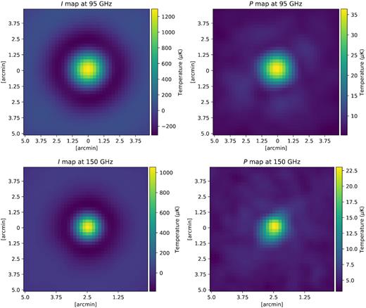
Stacked I and P cut-out maps extracted from the SPTpol 95 GHz (top panels) and 150 GHz (bottom panels) data at the positions of 69 sources with S > 40 mJy in the SPT–SZ 150 GHz catalogue described in Section 2.1.
3.2 Noise bias correction
Magnitudes such as P are naturally biased high by any noise in the estimate of Q or U. This bias becomes more significant at lower signal to noise. Handling this bias is thus critical to accurately measuring the polarization fraction of faint sources. In the literature, various methods have been developed to de-bias the polarization signal (e.g. Wardle & Kronberg 1974, and references therein). However, Simmons & Stewart (1985) have compared various de-biasing methods and concluded that all of them leave some residual bias at low signal to noise. In a recent study, Vidal, Leahy & Dickinson (2016) have shown that residual bias is smaller at low signal to noise if an independent and high signal-to-noise measurement of polarization angle is available.
3.3 Error bar estimation
We use the bootstrapping technique with replacement to estimate the uncertainties on measured 〈p2〉 values. Note that we neglect uncertainty in the measurement of the noise bias as the number of sources in a set is always much smaller than the number of random positions being used to estimate the noise bias. For each set of ns sources, we have an associated set of nsI, Q, and U map cut-outs from the matched filtered maps. We draw 10 000 random samples of ns map cut-outs from this set with replacement. For each of these 10 000 samples, we take the mean of the ns maps and determine the resulting p2 values. The standard deviation of these 10 000 mean p2 values is taken to be the uncertainty on the 〈p2〉 measurement for that set of sources.
3.4 Performance of the estimator
We test that we recover de-biased values for 〈p2〉 by injecting sets of simulated sources at random positions in the real matched filtered SPTpol I, Q, and U maps. All known sources in the SPT–SZ catalogue with 150 GHz flux |$S_{\rm 150\, GHz} \ge 6$| mJy are masked, and simulated sources are not injected into the masked areas. Seven thousand sources are injected, which is approximately 10 times larger than the actual sample size. The fluxes of the injected sources are drawn from the dN/dS distribution of the SPT–SZ sources (E19). A random polarization angle is assigned to each source. All of the injected sources are taken to have the same polarization fraction |$p_{\mathrm{ in}} = 0.03 ~(p_{\mathrm{ in}}^2 = 0.0009)$|. The injected sources are convolved by the SPTpol beam before being added to the real maps.
As shown in Fig. 2, the 〈p2〉 estimator accurately recovers the input value, |$p_{\mathrm{ in}}^2 = 0.0009$|, within the statistical uncertainties of the simulated sample. The green points demonstrate the effect of the noise bias, which is much larger than the signal for objects with fluxes ≲40 mJy at 95 and 150 GHz. However, even for the faintest objects at 95 GHz where the noise bias can be two times larger than the input polarization signal, the de-biased estimate is consistent with the input value. As laid out in Section 3.3, uncertainties are estimated from the measured p2 distribution of the simulated sample. We note that the plotted uncertainties are for a sample that is approximately 10 times larger than the real sample, and thus the uncertainties are three times smaller than the real, noise-only uncertainty.
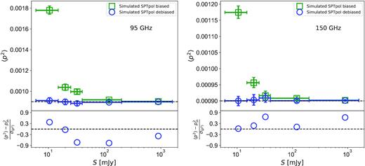
Simulation results showing the recovered 〈p2〉 from the simulated maps at 95 (left-hand panels) and 150 GHz (right-hand panels), where sources are injected with a constant input |$p_{\rm in}^2=0.0009$| (the solid black line) and random polarization angles. We inject ∼7000 sources to which flux is assigned using the measured dN/dS distribution. The simulated maps are created from observed matched filtered SPTpol maps by masking all point sources, which allows us to create simulated maps with same noise properties as in the observed maps. The recovered mean of the biased and de-biased 〈p2〉 values are shown as the green and blue data points, respectively, in different flux bins where the horizontal bars on data points represent bin size and the vertical error bars are computed using bootstrapping. The lower panels show the ratio of the difference between the recovered and input p2 value to the estimated uncertainty. The recovered value of p2 is consistent with the input in all flux bins within 1σ at both 95 and 150 GHz. Given that the simulated sample is 10 times larger than the real source sample, this sets a 68 per cent CL upper limit on the magnitude of any bias to be <0.35σ for the real data.
To better visualize any residual bias in our estimator, the lower panel of Fig. 2 shows the difference between the input and measured p2 values, in units of the 1σ uncertainties on the measurement in simulations. The agreement is excellent for all flux bins, showing no signs of systematic bias in the recovered polarization fraction. Given that these simulated uncertainties are approximately three times smaller than the real uncertainties, this sets a 68 per cent CL upper limit that the magnitude of any bias is <0.35σ for the real data. We conclude that there is no evidence for bias in the measurement of the mean square polarization fraction, 〈p2〉.
4 RESULTS
Applying the methods of Section 3 to the SPTpol maps at the SPT–SZ source locations yields a significant detection of the fractional source polarization, as would be expected from Fig. 1. When stacking the full source sample without any flux weighting, we find 〈p2〉 = [7.2 ± 1.9] × 10−4 for 95 GHz and 〈p2〉 = [5.3 ± 1.7] × 10−4 for 150 GHz. Weighting by flux yields a slight improvement in signal to noise. In this case, we find 〈p2〉 = [8.9 ± 1.1] × 10−4 for 95 GHz and 〈p2〉 = [6.9 ± 1.1] × 10−4 for 150 GHz over the whole sample. The results are summarized in Table 1. Given the high significance detection, we now turn to considering possible trends with source properties.
Mean-squared polarization fractions (〈p2〉) and inferred fractional polarization (|$\sqrt{\langle p^2 \rangle }$|) measurements for Nsource number of SPT–SZ selected sources stacked in flux bins Srange using 95 and 150 GHz SPTpol maps. There are four sources missing at 95 GHz due to smaller inverse noise variance weights at map edges. We show the unweighted (without any flux weighting) mean values for whole flux range as well. The error bars are evaluated using bootstrapping. We also show the flux weighted mean values, which is the best-fitting intercept, assuming zero slope for a straight line model fit to the mean-squared polarization fraction in five flux bins (see Section 4.1).
| Srange|$\rm [mJy]$| | Nsource | 〈p2〉 [10−4] | |$\sqrt{\langle p^2 \rangle }$| [10−2] |
|---|---|---|---|
| 95 GHz | |||
| 6 − 15 | 486 | 12.6 ± 6.4 | 3.56 ± 0.82 |
| 15 − 25 | 79 | 8.9 ± 3.8 | 2.98 ± 0.58 |
| 25 − 40 | 49 | 10.2 ± 2.9 | 3.18 ± 0.43 |
| 40 − 200 | 53 | 9.8 ± 1.9 | 3.13 ± 0.31 |
| 200 − 1500 | 15 | 6.3 ± 2.1 | 2.51 ± 0.40 |
| Unweighted mean | |||
| 6 − 1500 | 682 | 7.2 ± 1.9 | 2.68 ± 0.36 |
| Weighted mean | |||
| 6 − 1500 | 682 | 8.9 ± 1.1 | 2.98 ± 0.19 |
| 150 GHz | |||
| 6 − 15 | 490 | 9.4 ± 3.9 | 3.07 ± 0.58 |
| 15 − 25 | 79 | 4.3 ± 1.5 | 2.08 ± 0.35 |
| 25 − 40 | 49 | 7.6 ± 2.2 | 2.76 ± 0.37 |
| 40 − 200 | 53 | 9.4 ± 2.1 | 3.07 ± 0.34 |
| 200 − 1500 | 15 | 4.5 ± 1.8 | 2.12 ± 0.41 |
| Unweighted mean | |||
| 6 − 1500 | 686 | 5.3 ± 1.7 | 2.30 ± 0.34 |
| Weighted mean | |||
| 6 − 1500 | 686 | 6.9 ± 1.1 | 2.63 ± 0.22 |
4.1 Trends with flux and observing frequency
An important question about the polarized foreground emission in CMB surveys is whether the polarization fraction varies with flux or observing frequency. To answer these questions, we split the sample into five flux bins according to the SPT–SZ 150 GHz flux, and measure the mean-squared polarization fraction in each bin. The results are listed in Table 1 and shown in Fig. 3. The horizontal bars in the figure represent the range of fluxes in each bin.

Estimated 〈p2〉 for extragalactic radio sources at 95 (left-hand panel) and 150 GHz (right-hand panel). The blue data points represent de-biased 〈p2〉 values in five flux bins split according to the SPT–SZ 150 GHz flux in both panels. The horizontal bars on data points represent bin size and the vertical error bars are computed using bootstrapping (see Section 3.3). For comparison, we also show the squared values of polarization fraction 〈p〉2 measured by Bonavera et al. (2017a) and Trombetti et al. (2018) both at 100 (left-hand panel) and 143 GHz (right-hand panel) and Datta et al. (2018) (at 148 GHz in the right-hand panel) for high-flux radio sources.
Unsurprisingly, the uncertainties on the polarization fraction increase towards lower fluxes even though the sample size increases in this direction. This trend is due to the uncertainty on the noise bias; effectively at lower fluxes, the estimator approaches the limit of subtracting two large numbers to find a small difference.
To test whether the polarization fraction depends on the source flux, we fit a straight line (〈p2〉 = a + b × S) to the measured 〈p2〉 across the five flux bins at both 95 and 150 GHz. We use Markov Chain Monte Carlo and Gaussian likelihood for this. The polarization fraction measurements are assumed to be uncorrelated between different flux bins. Therefore, we model the covariance matrix as a diagonal matrix with entries given by the variance estimated through bootstrapping as discussed in Section 3.3. At 95 GHz, we find the best-fitting value for the offset is a = [9.7 ± 1.4] × 10−4, with a slope of b = [−0.38 ± 0.36] × 10−6. The results at 150 GHz are similar: the preferred offset is a = [6.9 ± 1.3] × 10−4 and the slope is b = [−0.24 ± 0.27] × 10−6. We show both sets of parameter constraints in Fig 4. Both slopes are within 1σ of zero; the measured 〈p2〉 does not show a statistically significant dependence on flux.
![We find no evidence that the polarization fraction depends on the flux of the source at either 95 or 150 GHz. Here, we show the 1σ and 2σ contours from fitting the measured 〈p2〉 values to a linear function of flux, 〈p2〉 = a + b × S, over the flux range S ∈ [6, 1500] mJy. The slope is consistent with zero at both frequencies. The shape of the degeneracy between the offset and slope can be understood by the fact the polarization fraction is well measured for bright sources, but increasingly uncertain towards lower fluxes. The errors at 95 GHz are larger due to higher map noise levels (see Section 2.2).](https://oup.silverchair-cdn.com/oup/backfile/Content_public/Journal/mnras/490/4/10.1093_mnras_stz2905/1/m_stz2905fig4.jpeg?Expires=1750488159&Signature=yHGhIpsxp8pRQOXWjy7R~uF1ypp5aZZ6CnLObDZzlrqs2GpjBHb5dSSqaRV4xvaugi642oDKDrxfUEjE9SCyMiDscrGcWlpp1HbD-jxOMkuNW0gT~yjxGpvH4LyzxJkssEUkH~gVLAIurBe08o5Zdu2jnhE2snbF955NArl19AugI9E2STYDIy276YD2zXSv3Y22vHjHhpufNOvpsbINv7ajDWYNyyN4i8JFlA5VPgFZbC76Kzy~5nk0L~e1jTb4VLw7VPw6L8ZI8QpFGEqZKUl7H~SWHmFg4nMH15eUSSFPeEu~kg3TMkxmmuDDEq4O1vZlHf-z~HkebByNFhqOWA__&Key-Pair-Id=APKAIE5G5CRDK6RD3PGA)
We find no evidence that the polarization fraction depends on the flux of the source at either 95 or 150 GHz. Here, we show the 1σ and 2σ contours from fitting the measured 〈p2〉 values to a linear function of flux, 〈p2〉 = a + b × S, over the flux range S ∈ [6, 1500] mJy. The slope is consistent with zero at both frequencies. The shape of the degeneracy between the offset and slope can be understood by the fact the polarization fraction is well measured for bright sources, but increasingly uncertain towards lower fluxes. The errors at 95 GHz are larger due to higher map noise levels (see Section 2.2).
We can also ask if the measured 〈p2〉 varies with observing frequency from 95 to 150 GHz. The measured offsets from the linear fits are consistent with no dependence on the observing frequency, with the best-fitting values differing by only 1.5σ. We can reduce these uncertainties by fitting a constant (i.e. fixing b = 0) to the five flux bins. We find best-fitting offsets of a = [8.9 ± 1.1] × 10−4 at 95 GHz and a = [6.9 ± 1.1] × 10−4 at 150 GHz. As shown in Table 1, these values are consistent with (and have slightly smaller error bars than) the results for the unweighted (without any flux weighting) stack of the full sample. The reduction in uncertainty can be understood by the weighting: in all stacks in this work, every source in the stack has equal weight. Splitting the data by flux bins weights the higher signal-to-noise high-flux sources more heavily. Given the best-fitting offsets differ by only 1.3σ, we conclude that the data are consistent with the hypothesis that the polarization fraction is the same at both frequencies.
4.2 Radio and dusty sources
As mentioned in Section 1, extragalactic sources that are bright at CMB frequencies are classified into two categories: radio sources (AGN) and dusty sources (DSFGs). Although both populations affect the measurements of CMB E & B modes of polarization, it is interesting to compare the polarization properties of these classes of sources separately. As described in Section 2.1, approximately 92 per cent of point sources with S150 ≥ 6 mJy observed in SPT–SZ survey are AGN, thus most of the signal in the stack of the whole sample is coming from them. Stacking just radio sources we find unweighted 〈p2〉 = [7.3 ± 2.0] × 10−4 and [5.2 ± 1.8] × 10−4 at 95 and 150 GHz, respectively. The uncertainties are the same as for the full sample as most of the DSFGs in the sample are low-flux sources. Similar to Section 4.1, fitting a constant (with slope fixed to zero) to this subsample of radio sources in five flux bins gives flux weighted 〈p2〉 = [8.9 ± 1.1] × 10−4 and [6.9 ± 1.1] × 10−4 at 95 GHz and 150 GHz, respectively. These unweighted and weighted numbers are consistent with the values obtained from whole sample as listed in Table 1.
The sample includes 55 sources classified as dusty sources in SPTpol observing region with S150 ≥ 6 mJy, based on the spectral index from 150 to 220 GHz. All of these dusty sources have 150 GHz flux below S = 35 mJy, and 93 per cent of them are in the lowest flux bin of this work (S ≤15 mJy). For dusty sources, we find unweighted 〈p2〉 to be consistent with zero with large error bars, i.e. 〈p2〉 = [51 ± 59] × 10−4 and [8.1 ± 9.2] × 10−4 at 95 and 150 GHz, respectively. The resulting 95 per cent confidence level upper limits are 〈p2〉95 < 16.9 × 10⁻³ and 〈p2〉150 < 2.6 × 10⁻³.
4.3 Comparison to previous results
The results shown in Table 1 are consistent with previous studies of AGN and DSFGs. Briefly, in previous studies, polarization fraction is found to be independent of flux (Battye et al. 2011; Trombetti et al. 2018; Datta et al. 2018) and frequency (Battye et al. 2011; Galluzzi et al. 2017; Bonavera et al. 2017a; Galluzzi et al. 2018; Trombetti et al. 2018) at GHz frequencies, and overall mean 〈p〉 is estimated at a level around 1−5 per cent, which are all consistent with our findings in this work. For comparison, we show the squared values of polarization fraction 〈p〉2 from Bonavera et al. (2017a) and Trombetti et al. (2018) (at 100 and 143 GHz Planck frequencies) in both panels of Fig 3. In the right-hand panel, we also show 〈p〉2 measured by Datta et al. (2018) at 148 GHz ACTpol observing frequency. Even though, these previous studies at high frequencies were performed for the brightest sources observed in separate CMB polarization experiments and by using different estimators for noise bias correction, we find 〈p〉2 estimated in these studies in good agreement with our 〈p2〉 measurements at both frequencies.
On the dusty side, Bonavera et al. (2017b) used Planck data to study ∼4700 dusty sources selected at 857 GHz with S ≥ 791 mJy (a flux threshold that is approximately comparable to this work when extrapolated to 150 GHz). For these dusty sources, they found 3.52 ± 2.48, 3.10 ± 0.75, and 3.65 ± 0.66 per cent polarization fraction at 143, 217, and 353 GHz, respectively. Using a different method and sources selected at 353 GHz with S ≥ 784 mJy, Trombetti et al. (2018) set 90 per cent CL upper limits on the polarization fraction of 〈p〉 < 0.039 at 217 GHz and 〈p〉 < 0.022 at 353 GHz. Comparing these with our measurements at 95 and 150 GHz from the last section, we see a trend of decreasing upper limits on the polarization fraction with increasing frequency, possibly due to larger signal to noise of dusty sources at higher frequencies. The upper limits on dusty sources at 150 GHz from the last section are compatible with the Bonavera et al. (2017b) measurements.
5 IMPLICATIONS FOR CMB MEASUREMENTS
Polarized emission from AGN and DSFGs can contaminate measurements of CMB E & B modes on small angular scales (high-ℓ). The polarized power from these objects, especially in the case of AGN, can be substantially reduced by masking the brightest sources. However, there are practical limits on how many sources can be masked, both because of the detection threshold in an experiment and because the fraction of the map that is masked naturally rises as the mask flux threshold is lowered. Thus, some residual polarized power from AGN and DSFGs will always remain in measurements of the CMB E and B mode power spectra. The measurement of the mean-squared polarization fraction in this work provides a direct means to predict this residual polarized power as a function of the masking threshold.
For AGN, we calculate the expected |$C_{\ell }^{\mathrm{ TT}}$| as a function of the masking threshold according to the source flux distribution dN/dS of the C2Ex model (Tucci et al. 2011) at 150 GHz. The C2Ex model builds on earlier models by, e.g. de Zotti et al. (2005) and is constructed by extrapolating the differential number counts of extragalactic sources observed at ∼5 GHz (see De Zotti et al. 2010) to higher frequencies. Tucci et al. (2011) also compare the modelled number counts to the observed number counts in the SPT (Vieira et al. 2010), the ACT (Marriage et al. 2011), and the Planck (Planck Collaboration VII 2011) surveys. Mocanu et al. (2013) compared the C2Ex model to observed point source counts in 720 deg2 SPT–SZ survey and found it consistent with sources above 80 mJy and below 20 mJy. The C2Ex model predicts |$D_{\ell =3000, \rm PS}^{TT} = 0.4 \, (11.4)\, \mu {\rm K}^2$| for a masking threshold of 2 (50) mJy at 150 GHz. We scale these powers to 95 GHz using a spectral index of -0.9, which is the value preferred in George et al. (2015). This predicts radio power of |$D_{\ell =3000, \rm PS}^{\mathrm{ TT}} = 1.1 \, (28.6)\, \mu {\rm K}^2$| for the same masking thresholds: 2 (50) mJy.
Fig. 5 shows the predicted power spectrum (Dℓ = ℓ(ℓ + 1)Cℓ/2π) at 95 GHz (left-hand panel) and 150 GHz (right-hand panel). The plots show the cosmological CMB EE and BB power spectra as well as the polarized power predicted for AGN (at two possible flux cut limits) and DSFGs, given the polarization fractions measured in this work. These figures illustrate that the polarized power from AGN and DSFGs will significantly contaminate measurements of the cosmological EE and BB power spectra only on the smallest angular scales. The main uncertainty in both panels is the polarization fraction of the DSFGs. We use the DSFG 〈p2〉 measured at 150 GHz for both 95 and 150 GHz. Given that both frequencies are in the extreme Rayleigh tail of the dust blackbody spectrum, we do not expect a significant shift in the sources probed or in the polarization of each source between 95 and 150 GHz. Supporting this position, Bonavera et al. (2017b) found the DSFG 〈p〉 to not vary with frequency from 143 to 353 GHz. For a reasonable mask flux threshold of 2 mJy, which is achievable by existing experiments like SPT-3G, the total polarized foreground power is less than the EE power spectrum out to ℓ ≲ 5700 (ℓ ≲ 4700) and the BB lensing power spectrum out to ℓ ≲ 5300 (ℓ ≲ 3600) at 95 (150) GHz.
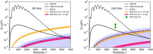
CMB polarization surveys will be minimally impacted by polarized source power after masking radio and dusty galaxies above reasonable flux thresholds. The predicted AGN power at 95 GHz (left-hand panel) and 150 GHz (right-hand panel) for the 〈p2〉 measured in this work is shown by the solid red (yellow) line for a 50 (2) mJy masking flux threshold in temperature. The filled area represents the 1σ uncertainties on 〈p2〉 (no uncertainty in the source distribution has been included). The dashed blue line and the filled blue area show the mean and the 1σ upper limit on the predicted DSFG polarized power, respectively. We have assumed that the fractional polarization of the DSFGs remains constant from the value measured at 150 GHz down to 95 GHz. The total polarized foreground power will be less than the CMB EE power spectrum out to ℓ ≲ 5700 (ℓ ≲ 4700) and CMB lensing BB power spectrum out to ℓ ≲ 5300 (ℓ ≲ 3600) at 95 (150) GHz. The green arrow in the right-hand panel shows the 95 per cent CL upper limit from the recent SPTpol EE power spectrum measurement (Henning et al. 2018). The polarization fraction measurements in this work support the expectation that extragalactic foregrounds will be fractionally smaller for CMB polarization than temperature measurements, thus allowing more modes to be used in polarization analyses.
The equivalent angular multipole for temperature is ℓ ∼ 4000 and ℓ ∼ 3100 at 95 and 150 GHz, respectively – more modes will be available to cosmological studies in polarization than temperature.
Note that the results are not particularly sensitive to the flux cut since the polarized foreground power envelope is being driven by DSFGs. The DSFG intensity power varies slowly with mask threshold since most DSFGs are fainter than 2 mJy. It is also worth noting that better measurements of the DSFG 〈p2〉 are likely to make the AGN power, and thus masking threshold, somewhat more important. We have reasons to believe that the polarization of DSFGs is lower than AGN, but 1σ limits in this work are higher (at 150 GHz) for DSFGs due to the limited number of DSFGs in the sample.
The inferred power from the measured 〈p2〉 values in this work are compatible with current observational constraints. Using the measured EE bandpowers from the SPTpol survey at 150 GHz, Henning et al. (2018) places a 95 per cent confidence level upper limit of |$D_{\ell =3000}^{\rm PS}\,\,\lt\,\, 0.107\,$||$\mu \rm K^2$| on polarized point source contribution to the EE power spectrum. This result is for a flux mask threshold of 50 mJy. The predicted power in our analysis is |$D_{\ell =3000}^{\rm PS}\,\, \lt\,\, 0.0092$||$\mu \rm K^2$| at 150 GHz, well below the observed upper limit. The other polarization fraction measurements discussed in Section 4.3 such as Datta et al. (2018) also argue for similar, low levels of polarized foreground power.
6 CONCLUSIONS
We present a new method to measure the mean-squared polarization fraction of sources in CMB surveys. We apply the method to 95 and 150 GHz maps from the SPTpol 500 deg2 survey at the locations of sources selected to have S150 ≥ 6 mJy in the SPT–SZ survey, and find 〈p2〉 for five flux bins. The flux-weighted mean-squared polarization fraction, i.e. the best-fitting value across the five bins is 〈p2〉95 = [8.9 ± 1.1] × 10−4 and 〈p2〉150 = [6.9 ± 1.1] × 10−4. We find no evidence in the current data that the polarization fraction varies with observing frequency or source flux density.
We split the source sample into DSFGs and AGN based on the observed spectral index from 150 to 220 GHz (Everett et al., in preparation). At 150 GHz, we find 〈p2〉AGN = [5.3 ± 1.7] × 10−4 and 〈p2〉DSFG = [8.1 ± 9.2] × 10−4 without any flux weighting. The larger uncertainties for the DSFG sample are due to the limited number of DSFGs above 6 mJy at 150 GHz. We use these measured mean-squared polarization fractions to predict the extragalactic foreground contribution to the CMB polarization power spectra.
Given the 1σ upper limit on the 〈p2〉 measured at 150 GHz in this work, the extragalatic foreground power will be subdominant to the CMB E mode power spectrum for ℓ ≲ 5700 (ℓ ≲ 4700) and to the CMB B-mode power spectrum for ℓ ≲ 5300 (ℓ ≲ 3600) at 95 (150) GHz.
These are lower limits on angular multipoles and most likely the CMB polarization power spectra will dominate out to even higher multipoles. In comparison, these extragalactic foregrounds surpass the CMB temperature power spectrum around ℓ ∼ 4000 and ℓ ∼ 3100 at 95 and 150 GHz, respectively, for the same flux cuts. With the exquisitely low noise levels expected for current and upcoming experiments like SPT-3G (Bender et al. 2018) and CMB-S4 (Abazajian et al. 2016), we will thus be able to recover more cosmological information from CMB polarization anisotropies than temperature anisotropies by virtue of going to much smaller angular scales.
ACKNOWLEDGEMENTS
South Pole Telescope (SPT) is supported by the National Science Foundation through grant PLR-1248097. Partial support is also provided by the NSF Physics Frontier Center grant PHY-1125897 to the Kavli Institute of Cosmological Physics at the University of Chicago, the Kavli Foundation, and the Gordon and Betty Moore Foundation grant GBMF 947. This research used resources of the National Energy Research Scientific Computing Center (NERSC), a DOE Office of Science User Facility supported by the Office of Science of the U.S. Department of Energy under Contract No. DE-AC02-05CH11231. The Melbourne group acknowledges support from the Australian Research Council’s Discovery Projects scheme (DP150103208).
Footnotes
In practice, we found nearly identical results (<0.1σ difference in 〈p2〉) when masking all sources as in the procedure described here, suggesting that any noise variation is negligible.
