


ABSTRACT
Spectropolarimetry enables us to measure the geometry and chemical structure of the ejecta in supernova explosions, which is fundamental for the understanding of their explosion mechanism(s) and progenitor systems. We collected archival data of 35 Type Ia supernovae (SNe Ia), observed with Focal Reducer and Low-Dispersion Spectrograph (FORS) on the Very Large Telescope at 127 epochs in total. We examined the polarization of the Si ii λ6355 Å line (|$p_{\rm Si\, \small {II}}$|) as a function of time, which is seen to peak at a range of various polarization degrees and epochs relative to maximum brightness. We reproduced the |$\Delta m_{15}\!-\!p_{\rm Si\, \small {II}}$| relationship identified in a previous study, and show that subluminous and transitional objects display polarization values below the |$\Delta m_{15}\!-\!p_{\rm Si\, \small {II}}$| relationship for normal SNe Ia. We found a statistically significant linear relationship between the polarization of the Si ii λ6355 Å line before maximum brightness and the Si ii line velocity and suggest that this, along with the |$\Delta m_{15}\!-\!p_{\rm Si\, \small {II}}$| relationship, may be explained in the context of a delayed-detonation model. In contrast, we compared our observations to numerical predictions in the |$\Delta m_{15}\!-\!v_{\rm Si\, \small {II}}$| plane and found a dichotomy in the polarization properties between Chandrasekhar and sub-Chandrasekhar mass explosions, which supports the possibility of two distinct explosion mechanisms. A subsample of SNe displays evolution of loops in the q–u plane that suggests a more complex Si structure with depth. This insight, which could not be gleaned from total flux spectra, presents a new constraint on explosion models. Finally, we compared our statistical sample of the Si ii polarization to quantitative predictions of the polarization levels for the double-detonation, delayed-detonation, and violent-merger models.
1 INTRODUCTION
Type Ia supernovae (SNe Ia) are used as standard candles (after applying proper scaling relations; see Pskovskii 1977; Phillips 1993) to measure the expansion rate of the Universe (Riess et al. 1998; Perlmutter et al. 1999). The ultimate future goal is to constrain the nature of dark energy, which requires accurate measurements of the equation-of-state parameter w.
Several upcoming sky surveys that are expected to discover SNe at a very high cadence will lead to an improvement in the statistics and advances in SN Ia cosmology. The Large Synoptic Survey Telescope (LSST) alone is expected to observe 50 000 SNe Ia per year with an adequate time coverage for cosmological distance estimates (LSST Science Collaboration 2009). Furthermore, future space missions will enable us to extend the SN Ia Hubble diagram to redshifts above z ∼ 2 and up to z ∼ 4 using the James Webb Space Telescope (Hook 2013; Spergel et al. 2015; Wang et al. 2017). Even with a large statistical sample, it is demanding to accurately measure the equation-of-state parameter w, due to systematic errors. It is known that SNe Ia are exploding carbon/oxygen (C/O) white dwarfs close to the Chandrasekhar mass limit; however, their evolutionary path and the exact progenitor system are still not known. Identifying the SN Ia progenitors is important, because we need to understand the evolution of their luminosity with cosmic time, depending on metallicity, age, dust, etc. (Riess & Livio 2006).
The three most popular SN Ia progenitor systems are the single-degenerate model, in which a white dwarf accretes material from a non-degenerate companion until it reaches the Chandrasekhar mass and explodes; the double-degenerate model in which two white dwarfs merge smoothly or violently; and the core-degenerate progenitor model (Kashi & Soker 2011) in which a white dwarf merges with the core of a giant companion star (see Livio & Mazzali 2018, for a SN Ia review).
One approach to learn more about the progenitor system is to investigate the environment of the SNe, because different progenitor models can imply different environments. Spectropolarimetry offers an independent method to the study inter/circumstellar dust properties (by observing the continuum polarization) and the analysis of the 3D geometrical properties of unresolved sources (by observing the intrinsic continuum polarization and polarization across spectral lines). The latter provides insights into global and local asymmetries of SN explosions (see Shapiro & Sutherland 1982; Höflich 1991; Spyromilio & Bailey 1993; Trammell, Hines & Wheeler 1993; Wang et al. 1996). These aspects are fundamental for our understanding of the phenomenon and are hardly approachable by any other observational technique (Wang & Wheeler 2008; Branch & Wheeler 2017).
In this work, we primarily focus on the linear polarization in the absorption lines, particularly the λ6355 Å silicon line, because it is the most prominent polarized line, along with the Ca ii triplet. However, this latter feature occurs in the low signal-to-noise ratio (SNR) wavelength range of our observations. We use a statistical sample of 35 SNe Ia observed with FORS1 (before 2005) and FORS2, mounted at the Cassegrain focus of ESO’s Very Large Telescope (VLT), to explore the polarization across the spectral lines, look for relationships between the Si ii line velocity and polarization degree, and compare our polarization measurements with predictions from simulations with the main aim to constrain the SN Ia explosion mechanism and progenitor system. Additionally, because our sample includes a number of objects affected by low or negligible reddening, we derive an upper limit on the intrinsic continuum polarization.
To understand the polarization spectra observed towards SN Ia sightlines, it is important to understand the mechanisms of polarization, which are presented in Section 2. In Section 3, we explain the instruments, observations, and our sample of SNe Ia; in Section 4, we explain the methods used to reduce the data; in Section 5, we show and discuss the results; and in Section 6, we summarize the main results and provide conclusions.
2 POLARIZATION MECHANISMS
2.1 Continuum polarization
There are three continuum polarization mechanisms, relevant for the SN Ia observations, that we need to consider:
Polarization produced due to linear dichroism in non-spherical grains: When light passes through the interstellar medium, or a cloud of non-spherical supramagnetic dust grains, which are aligned with the galactic magnetic field, the electric vector of the light wave parallel to the major axis of the dust grains will experience higher extinction than light waves parallel to the minor axis of the dust grain, and thus we will observe a net polarization (van de Hulst 1957; Martin 1974; Shapiro 1975).
The Serkowski curve (Serkowski, Mathewson & Ford 1975) is an empirical wavelength dependence derived using a sample of Milky Way stars observed in the optical wavelength range (see also Wilking et al. 1980; Wilking, Lebofsky & Rieke 1982; Whittet et al. 1992), which is used to characterize interstellar linear polarization curves:where the wavelength of peak polarization, λmax, in general depends on the dust grain size distribution. For an enhanced abundance of small dust grains, λmax moves to shorter wavelengths, and for an enhanced abundance of large dust grains to longer wavelengths. pmax is the peak degree of polarization, and K depends on the width of the curve. Narrow curves will have large K values, compared to wide curves that have small K values. Serkowski et al. (1975) also found that RV ≈ 5.5λmax, where λmax is in |$\mu \mathrm{ m}$| and RV is the total-to-selective extinction ratio, RV = A(V)/E(B − V).(1)$$\begin{eqnarray*} \frac{p(\lambda)}{p_{\mathrm{\rm max}}} = \exp \left[-K \,\mathrm{ln}^2 \left(\frac{\lambda _{\mathrm{\rm max}}}{\lambda } \right) \right] , \end{eqnarray*}$$- Polarization by scattering from nearby material: Single scattering from nearby dust clouds or sheets produces polarized light perpendicular to the scattering plane (see White 1979a,b; Wang & Wheeler 1996). The polarization curve produced by scattering is given bywhere cR is the amplitude of the scattering (e.g. cR = 0.027 ± 0.002 per cent in Andersson et al. 2013). The index of the power law is not well constrained, and is usually chosen to be −4, appropriate for both Rayleigh scattering from polarizable molecules and Mie scattering in the small grain limit (Andersson et al. 2013). Note that equation (2) is only valid in case of low optical depth. In case of large optical depths, the blue part is strongly depleted, because of multiple scattering, which is more probable in the blue part of the spectrum where scattering is more efficient (see Nagao, Maeda & Tanaka 2018).(2)$$\begin{eqnarray*} p(\lambda) = c_\mathrm{ R} \times \lambda ^{-4}, \end{eqnarray*}$$
Patat et al. (2015) found that highly reddened SNe with low total-to-selective extinction ratios, RV, also have peculiar continuum polarization curves steeply rising towards the blue part of the spectrum, and with polarization peaks |$\lambda _{\rm max} \lesssim 0.4 \, \mu {\rm m}$|. It is not fully understood whether such polarization curves are produced by small interstellar grains in their host galaxies or by scattering from nearby circumstellar material. For more information on interstellar (or circumstellar) continuum polarization towards SNe Ia, see Patat et al. (2015), Zelaya et al. (2017), Cikota et al. (2017b), Hoang (2017), Cikota et al. (2018), and Hoang et al. (2019).
Polarization induced by electron scattering in globally aspherical photospheres: In case of spherical photospheres, the intensity of scattered (linearly polarized) light from free electrons will be equal in orthogonal directions, and thus, we do not observe a net polarization (Fig. 1a). In the case of an aspherical photosphere, on the other hand, the net intensity of scattered light perpendicular to the major axis of the projected photosphere will be larger than the intensity of the scattered light perpendicular to the minor axis (Fig. 1b), and therefore, we will observe a net polarization (see Shapiro & Sutherland 1982; Höflich 1991). The intrinsic continuum polarization in SNe Ia is typically ≲0.4 per cent, which is consistent with global asphericities at the ∼10 per cent level (Chornock & Filippenko 2008). The highest intrinsic continuum polarization was observed in the subluminous Type Ia SN 1999by (Howell et al. 2001), which showed an intrinsic polarization of ∼0.8 per cent. Howell et al. (2001) found that the spectropolarimetric data could be modelled by an ellipsoid with an axial ratio of 1.17 seen equator-on.
Despite the Thomson scattering being wavelength independent, in some cases the intrinsic continuum polarization of SNe Ia decreases towards the blue end of the spectrum (see the subluminous SN 1999by and SN 2005ke; Patat et al. 2012). This is due to depolarization by a large number of bound–bound transitions, primarily of iron-peak elements (Pinto & Eastman 2000), in the UV and blue part of the spectrum (Chornock & Filippenko 2008). This can be explained by the probability of the last scattering of the photons due to electrons versus the probability of the last scattering due to lines. If the opacity is dominated by bound–bound scattering rather than electron scattering, the polarization will be suppressed. For a Fe-rich ejecta, line opacity dominates, and the importance of electron scattering is suppressed.
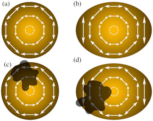
Illustration of the mechanism by which polarization arises. (a) In case of a spherical SN photosphere, we will observe a net polarization of p = 0. (b) In case of an aspherical photosphere, we will observe a net continuum polarization p > 0. (c) If there is an inhomogeneous distribution of material in front of the spherical photosphere, it will obscure part of the polarized light, and we will observe polarization across spectral lines only. (d) An aspherical photosphere with an inhomogeneous distribution of material in front of the photosphere would produce both continuum and line polarization.
2.2 Line polarization
As explained in the previous subsection, SN Ia explosions are in general globally spherical explosions (Section 2.1), which is also reflected in the spherical shapes of SN Ia remnants (e.g. Lopez et al. 2009). Polarization across spectral lines (hereafter line polarization) can give us insight into the geometry of the ejecta, which depends on the explosion scenario and/or the progenitor system. In Section 2.2.1, we explain line polarization predictions for different explosion scenarios, based on simulations, whereas here we focus on how line polarization is produced in general.
Fig. 1 shows a very simplified illustration of the mechanism by which polarization arises from the electron-scattering dominated photosphere. In the case of a spherical photosphere, there will be an equal amount of polarized light coming from all directions (Fig. 1a), and therefore, we will observe a net polarization of p = 0. However, if there is aspherically distributed material in front of the photosphere, it will obscure part of the polarized light from the photosphere, and thus, the cancellation of the perpendicular intensity beams will be incomplete and we will observe a net polarization, p > 0, in the polarization spectrum associated with the corresponding absorption line in the flux spectrum (Fig. 1c and d; see also Kasen et al. 2003; Wang et al. 2003).
Depending on the geometry and velocity distribution of the blocking material, different properties in the Stokes q–u plane1 will be observed. If the distribution of the absorbers (or clumps) is not spherically symmetric and does not have a common symmetry axis, and if there is a velocity-dependent range of position angles, we will observe a smooth change in the polarization angle, i.e. we will observe loops in the q–u plane as a function of wavelength. However, in case of an axisymmetric distribution of the ejecta (e.g. a torus or bipolar ejecta), we will observe a line in the q–u plane, but no loops, because in these configurations the geometry of the obscuring material shares the same symmetric axis as the photosphere (see Wang et al. 2001, 2003; Kasen et al. 2003; Wang & Wheeler 2008; Tanaka et al. 2017, for a more detailed explanation).
2.2.1 Line polarization predictions for different SN Ia explosion models
Bulla et al. (2016a) ran simulations to predict polarization signatures for the violent-merger model of Pakmor et al. (2012), which is presumed to be highly asymmetric, hence describing what can be considered as a limiting case. They found that the polarization signal significantly varies with the viewing angle. In the equatorial plane of the explosion, the continuum polarization levels will be modest, ∼0.3 per cent, while at orientations out of the equatorial plane, where the departures from a dominant axis are higher, the degrees of polarization will be higher (∼0.5–1 per cent). However, for all orientations, the polarization spectra display strong line polarization (∼1–2 per cent). They suggest that the violent-merger scenario may explain highly polarized events such as SN 2004dt (Bulla et al. 2016a).
In a similar study, Bulla et al. (2016b) predict polarization signatures for the double-detonation (DDET, from Fink et al. 2010) and delayed-detonation (DDT, from Seitenzahl et al. 2013) models of SNe Ia.
In the DDT model, a white dwarf near the Chandrasekhar mass, which accretes material from a non-degenerate companion, explodes after an episode of slow (subsonic) carbon burning (carbon deflagration) near the centre (Khokhlov 1991). In the DDET model, the explosion in the core of a sub-Chandrasekhar white dwarf is triggered by a shock wave following a detonation of a helium layer at the white dwarf’s surface, which has been accreted from a helium-rich companion star (Fink et al. 2010).
For both explosion models, Bulla et al. (2016b) predict modest degrees of polarization (≲1 per cent). The peak of the intrinsic continuum polarization of ∼0.1–0.3 per cent decreases after maximum brightness, and prominent polarization of the absorption features is present in the simulated spectra, in particular of the Si ii λ6355 Å line. The simulations show low polarization across the O i 7774 Å, which is consistent with the observed values in normal SNe Ia. The low polarization across O i reflects the fact that the oxygen is not a product of the dynamical thermonuclear burning, so that oxygen in the spectra comes from the primordial oxygen of the white dwarf (which is supposed to be spherically distributed; Wang et al. 2006; Patat et al. 2009). This is a very important result from polarimetry, placing a constraint on the explosion models (Höflich et al. 2006).
3 OBSERVATIONS AND DATA
3.1 Instruments and observations
Our targets were observed with the Focal Reducer and Low-Dispersion Spectrograph (FORS) in spectropolarimetric mode (PMOS), mounted on the Cassegrain focus of the VLT at Cerro Paranal in Chile (Appenzeller et al. 1998).
Two versions of FORS were built, and mounted to different VLT unit telescopes since the start of operations. FORS1 was installed on Antu (UT1) and commissioned in 1998, while FORS2 was installed on Kueyen (UT2) 1 year later. They are largely identical with a number of differences; particularly, the polarimetric capabilities were offered only on FORS1. In June 2004, FORS1 was moved to Kueyen (UT2) and FORS2 to Antu (UT1), and in August 2008 the polarimetric capabilities were transferred from FORS1 to FORS2.
FORS in PMOS mode is a dual-beam polarimeter, with a wavelength coverage from ∼330 to 1100 nm. It contains a Wollaston prism, which splits an incoming beam into two beams with orthogonal directions of polarization, the ordinary (o) and extraordinary (e) beams. The observations of the SNe Ia in this work were obtained with FORS1 or FORS2, a 300V grism, with and/or without the order separating GG435 filter. The GG435 filter has cut-off at ∼435 |$\mu {\rm m}$|, and is used to prevent second-order contamination. The effect of second-order contamination on spectropolarimetry is in most cases negligible, but can be significant for very blue objects (see appendix in Patat et al. 2010). The half-wave retarder plate was positioned at four angles of 0°, 22.5°, 45°, and 67.5° per sequence. The ordinary and extraordinary beams were extracted using standard procedures in IRAF (as described in Cikota et al. 2017a). Wavelength calibration was achieved using He–Ne–Ar arc lamp exposures. The typical rms accuracy is ∼0.3 Å. The data have been bias subtracted, but not flat-field corrected; however, the detector artefacts get reduced by taking a redundant number of half-wave positions (see Patat & Romaniello 2006).
Fossati et al. (2007) analysed observations of standard stars for linear polarization obtained from 1999 to 2005 with FORS1, in imaging (IPOL) and spectropolarimetric (PMOS) mode. They found a good temporal stability and a small instrumental polarization in PMOS mode. In a similar study, Cikota et al. (2017a) tested the temporal stability of the PMOS mode of FORS2 since it was commissioned, using a sample of archival polarized and unpolarized standard stars, and found a good observational repeatability of total linear polarization measurements with an rms ≲0.21 per cent. They also confirmed and parametrized the small (≲0.1 per cent) instrumental polarization found by Fossati et al. (2007), which we correct by applying their linear functions to Stokes q and u.
3.2 Supernova sample
In this work, we collected archival data2 of 35 SNe Ia, observed with FORS1 and FORS2 in spectropolarimetry mode, between 2001 and 2015, at 127 epochs in total. A list of the targets with some basic properties is provided in Table 1, while a full observing log is given in Table A1 (Supporting Information). The observations in Table A1 (Supporting Information) are grouped into individual epochs, separated by a space.
SN Ia sample.
| Name | z | TBmax (MJD) | Δm15 (mag) | Epochs (days relative to Tmax) | References (z, TBmax, Δm15) |
|---|---|---|---|---|---|
| SN 2001dm | 0.01455 | 52128.0 ± 10.0 | – | 6.3 | 1, estimate , – |
| SN 2001V | 0.01502 | 51972.58 ± 0.09 | 0.73 ± 0.03 | −10.4, −6.4, 17.5, 30.6 | 2, SNooPy, 3 |
| SN 2001el | 0.00364 | 52182.5 ± 0.5 | 1.13 ± 0.04 | −4.2, 0.7, 8.7, 17.7, 39.6 | 4, 5, 6 |
| SN 2002bo | 0.00424 | 52356.5 ± 0.2 | 1.12 ± 0.02 | −11.4, −7.4, −6.4, −4.5, −1.4, 9.6, 12.6 | 7, 5, 6 |
| SN 2002el | 0.02469 | 52508.76 ± 0.05 | 1.38 ± 0.05 | −8.6, −7.6 | 4, SNooPy, 3 |
| SN 2002fk | 0.007125 | 52547.9 ± 0.3 | 1.02 ± 0.04 | 0.4, 4.4, 13.4 | 8, 5, 6 |
| SN 2003eh | 0.02539 | 52782.0 ± 10.0 | – | 0.0, 12.0 | 9, estimate, – |
| SN 2003hv | 0.005624 | 52891.2 ± 0.3 | 1.09 ± 0.02 | 6.1 | 4, 5, 6 |
| SN 2003hx | 0.007152 | 52892.5 ± 1.0 | 1.17 ± 0.12 | 4.8, 16.8, 18.8 | 1, 10, 11 |
| SN 2003W | 0.018107 | 52679.98 ± 0.11 | 1.3 ± 0.05 | −8.7, −6.7, 16.1 | 4, SNooPy, 3 |
| SN 2004br | 0.019408 | 53147.9 ± 0.27 | 0.68 ± 0.15 | −3.9 | 4, SNooPy, 12 |
| SN 2004dt | 0.01883 | 53239.98 ± 0.07 | 1.21 ± 0.05 | −9.7, 4.4, 5.2, 10.3, 33.2 | 13, SNooPy, 3 |
| SN 2004ef | 0.028904 | 53264.4 ± 0.1 | 1.45 ± 0.01 | −5.3 | 4, 5, 6 |
| SN 2004eo | 0.015701 | 53278.51 ± 0.03 | 1.32 ± 0.01 | −10.4 | 2, 14, 6 |
| SN 2005cf | 0.006461 | 53533.94 ± 0.05 | 1.18 ± 0.01 | −11.9, −5.8 | 7, SNooPy, Wang (priv. comm.) |
| SN 2005de | 0.015184 | 53598.89 ± 0.05 | 1.41 ± 0.06 | −10.9, −4.9 | 2, SNooPy, 3 |
| SN 2005df | 0.004316 | 53599.18 ± 0.1 | 1.06 ± 0.02 | −10.8, −8.8, −7.8, −6.8, −2.8, 0.2, 4.2, 5.2, 8.2, 9.1, 29.2, 42.1 | 15, SNooPy, SNooPy |
| SN 2005el | 0.01491 | 53647.0 ± 0.1 | 1.4 ± 0.01 | −2.7 | 13, 5, 6 |
| SN 2005hk | 0.01306 | 53685.42 ± 0.14 | 1.47 ± 0.14 | −2.3, 11.7 | 16, SNooPy, 17 |
| SN 2005ke | 0.00488 | 53699.16 ± 0.08 | 1.66 ± 0.14 | −9.1, −8.1, 75.9 | 13, SNooPy, 17 |
| SN 2006X | 0.00524 | 53786.3 ± 0.1 | 1.09 ± 0.03 | −10.9, −9.0, −8.1, −7.1, −4.0, −3.0, −1.9, 37.9, 38.9 | 13, 5, 6 |
| SN 2007fb | 0.018026 | 54288.41 ± 0.17 | 1.37 ± 0.01 | 3.0, 6.0, 6.9, 9.9 | 18, SNooPy, SNooPy |
| SN 2007hj | 0.01289 | 54350.23 ± 0.1 | 1.95 ± 0.06 | −1.1, 4.9, 10.9 | 13, SNooPy, 12 |
| SN 2007if | 0.073092 | 54343.1 ± 0.6 | 1.07 ± 0.03 | 13.1, 20.1, 45.0, 46.0 | 4, 5, 6 |
| SN 2007le | 0.005522 | 54399.3 ± 0.1 | 1.03 ± 0.02 | −10.3, −5.1, 40.7 | 4, 5, 6 |
| SN 2007sr | 0.005417 | 54447.82 ± 0.24 | 1.05 ± 0.07 | 63.4 | 18, SNooPy, 12 |
| SN 2008ff | 0.0192 | 54704.21 ± 0.63 | 0.90 ± 0.06 | 31.0 | 19, 20, 21 |
| SN 2008fl | 0.0199 | 54720.79 ± 0.86 | 1.35 ± 0.07 | 2.2, 8.3, 9.2, 11.3, 15.3 | 22, 20, 21 |
| SN 2008fp | 0.005664 | 54730.9 ± 0.1 | 1.05 ± 0.01 | −5.6, −0.5, 1.4, 5.4 | 4, 5, 6 |
| SN 2010ev | 0.009211 | 55385.09 ± 0.14 | 1.12 ± 0.02 | −1.1, 2.9, 11.9 | 16, SNooPy, 23 |
| SN 2010ko | 0.0104 | 55545.23 ± 0.23 | 1.56 ± 0.05 | −7.1, −6.0, −2.0, −1.2, 1.9, 3.9, 10.9, 15.9, 50.9, 51.8, 57.8, 58.8, 59.8 | 24, SNooPy, SNooPy |
| SN 2011ae | 0.006046 | 55620.22 ± 0.39 | – | 4.0, 16.0 | 18, SNooPy, – |
| SN 2011iv | 0.006494 | 55905.6 ± 0.05 | 1.77 ± 0.01 | −0.4, 2.6, 5.6, 11.5, 12.5, 19.5 | 16, 25, 26 |
| SN 2012fr | 0.0054 | 56244.19 ± 0.0 | 0.8 ± 0.01 | −12.1, −6.9, 1.0, 23.1 | 27, SNooPy, SNooPy |
| SN 2015ak | 0.01 | 57268.13 ± 0.1 | 0.95 ± 0.01 | −13.1, 4.9, 6.9, 23.9 | Spec. fit, SNooPy, SNooPy |
Note: SNooPy: see Section 4.3; 1: Silverman et al. (2012); 2: Ganeshalingam, Li & Filippenko (2013); 3: Wang, Baade & Patat (2007); 4: Planck Collaboration (2016); 5: Dhawan et al. (2015); 6: Dhawan et al. (2015); 7: Mandel, Narayan & Kirshner (2011); 8: Amanullah et al. (2010); 9: Prieto, Stanek & Beacom (2008); 10: Misra et al. (2008); 11: Misra et al. (2008); 12: Ganeshalingam et al. (2010); 13: Folatelli et al. (2013); 14: Dhawan et al. (2015); 15: Yaron & Gal-Yam (2012); 16: Chomiuk et al. (2016); 17: Hicken et al. (2009); 18: Friedman et al. (2015); 19: Tan (2008); 20: Krisciunas et al. (2017b); 21: Krisciunas et al. (2017b); 22: Pignata et al. (2008); 23: Gutiérrez et al. (2016); 24: Leonini & Brimacombe (2010); 25: Gall et al. (2018); 26: Gall et al. (2018); 27: Buil (2012).
Fig. 2 shows the number of observed epochs per SN, and the distribution of observed epochs. Eight SNe have been observed at a single epoch, while the most frequently observed supernovae are SN 2010ko (observed at 13 epochs), SN 2005df (12 epochs), SN 2006X (9 epochs), SN 2002bo (7 epochs), and SN 2011iv (6 epochs).
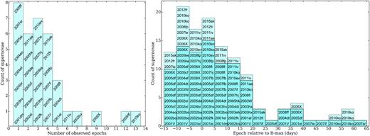
Left: Distribution of number of epochs per SN. For example, SN 2001el, SN 2004dt, and SN 2008fl have been observed at five epochs. Right: Distribution of observed epochs. For example, SN 2007if, SN 2012fr, and SN 2015ak have been observed between 20 and 25 days past peak brightness. The dark blue colour is the number of unique supernovae observed per epoch bin (note that some SNe were observed at multiple epochs within the same epoch bin).
Our sample also contains a few spectroscopically peculiar subluminous objects (see Taubenberger 2017, for a review of different sub-types). SN 2005ke is a 91bg-like object (Patat et al. 2012), SN 2005hk is a 2002cx-like object (Maund et al. 2010a), while SN 2011iv and SN 2004eo are transitional objects (see Gall et al. 2018; Pastorello et al. 2007, respectively). Also, a spectrum of SN 2007hj near maximum light shows similarities to several subluminous SNe Ia (Blondin et al. 2007).
4 METHODS
4.1 Stokes parameters, polarization degree, and polarization angle
The uncertainties on the normalized flux differences, the Stokes parameters, and the polarization and polarization angle were calculated by propagating the flux uncertainty (‘sigma spectrum’) of the ordinary and extraordinary beams, which were extracted, along with the beams, using the IRAF task apextract.apall.
4.2 Wavelet decomposition and continuum removal
In this paper, we mainly focus on line polarization, and do not investigate interstellar, circumstellar, or intrinsic continuum polarization. Therefore, we remove the whole continuum polarization without distinguishing between the three components (see Section 2.1).
For the purpose of a more general approach, we preferred a different method, which does not require the θISP to be determined and is also applicable to small levels of ISP. Therefore, to determine and subtract the continuum, we first perform an |$\rm \grave{a}$| trous wavelet decomposition (Holschneider et al. 1989) of the individual ordinary and extraordinary beams, which allows us to distinguish between the continuum spectra and the line spectra in a systematic way.
The wavelet decomposition is a method to decompose a function into a set of J scales, by convolving the function with a convolution mask with an increasing size. Assuming a convolution mask (e.g. the commonly used Mexican hat or simply a triangle), the first convolution is performed on the initial function c0(k), to generate c1(k). The difference c0(k) − c1(k) is the first wavelet scale w1(k). The algorithm is then reapplied j times, using a double-sized convolution mask, until scale J is reached (see also Wagers, Wang & Asztalos 2010).
Fig. 3 shows an example of a wavelet decomposition of a flux spectrum into a ‘continuum’ (sum of scales 9 + 10 + 11), ‘noise’ (scales 1 + 2 + 3), and the remaining spectrum (scales 4 + 5 + 6 + 7 + 8). Note that the ‘continuum’ does not necessarily coincide with the physical continuum of the SN. To determine the continuum-subtracted polarization spectra, we first calculate the total Stokes q and u by summing all wavelet scales of the individual ordinary and extraordinary flux spectra, except the first three in order to reduce the noise, and following the equations in Section 4.1. Then, we calculate the continuum Stokes q and u, using the ‘continuum’ spectra of the individual ordinary and extraordinary flux spectra, i.e. using the sum of the last three wavelet scales only. Finally, we subtract the continuum Stokes q and u from the total Stokes q and u. Note that, in general, the normalized Stokes parameters q and u are not additive (in contrast to unnormalized Stokes Q and U). However, the ISP cannot be expressed as a regular Stokes vector (I, Q, U, V), because the ISP does not carry any intensity, IISP. When a beam of radiation traverses the ISP, the Stokes vector is transformed and the process can be described as the product between the incoming Stokes vector and a Mueller matrix, which approximates a partial polarizer (see appendix B in Patat et al. 2010). In the case of weak incoming polarization, this corresponds to a vectorial sum between SSN(I, Q, U) and SISP(0, QISP, UISP), where Iout is attenuated by the extinction (Patat et al. 2010).
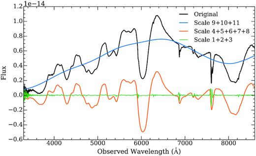
Example of an |$\rm \grave{a}$| trous wavelet decomposition. The black line is an original spectrum, and blue, orange, and green curves are the sum of the last three (9 + 10 + 11), first three (1 + 2 + 3), and middle five wavelet scales (4 + 5 + 6 + 7 + 8), respectively.
This also instantly removes the continuum polarization from the line photons (which may still contain some polarization due to interstellar or circumstellar scattering), assuming that the continuum polarization crossing the absorption lines is smoothly following the continuum polarization determined by wavelet decomposition of the flux spectra. An example of continuum subtraction from a polarization spectrum is shown in Fig. 4. The blue curves in the middle panels display the continuum Stokes q and u determined as described.

Example of continuum subtraction from a polarization spectrum of SN 2002bo at −1 day relative to peak brightness. The top panel shows the total degree of polarization (black curve) and the middle panels are Stokes q and u. The blue curves display the continuum polarization Stokes q and u determined with wavelet decomposition (middle panels) and the calculated continuum polarization from the Stokes parameters (top panel). The bottom panel shows the continuum-subtracted polarization spectrum, compared to the flux spectrum (red curve). The λ6355 Å Si ii line, at ∼6000 Å, displays two peaks, related to the high-velocity and photospheric silicon lines, respectively. The bin size of the polarization spectra is 25 Å, and the error bars represent 1σ uncertainties.
4.3 Light-curve fitting
For a number of SNe Ia, for which we did not find the date of peak brightness, Tmax, or the light-curve decline rate, Δm15 (Phillips 1993), in the literature, we downloaded light curves from the Open Supernova Catalog,3 which is an online collection of observations and metadata for SNe (Guillochon et al. 2017), and determined the missing parameters.
For this purpose, we fit the light curves using the SNooPy package (Burns et al. 2011, 2015), in order to determine the time of peak brightness, Tmax, and Δm15. SNooPy contains tools for the analysis of SN Ia photometry, and includes four models to fit the light curves. For our purpose, we used the ‘EBV_model’, which is based on the empirical method for fitting multicolour light curves developed by Prieto, Rest & Suntzeff (2006). Fig. 5 shows an example fit of SN 2005df observations.
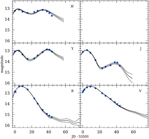
An example of light-curve fitting with SNooPy. Shown is a multicolour light-curve fit to SN 2005df observations in five passband filters (Krisciunas et al. 2017a). The derived light-curve parameters are Tmax = 53599.2 ± 0.1 MJD, E(B − V)Host = 0.024 ± 0.012 mag, and Δm15 = 1.06 ± 0.02 mag. The date on the x-axis is in units of days relative to an arbitrary zero-point. The solid line is the best-fitting line, and the dashed lines are the 1σ uncertainties. Note that the B and V measurements at 53700 MJD (Krisciunas et al. 2017a) are outside of the axes.
A list of SNe Ia for which we fit their light curves, including the number of photometric observations used per passband filter and the corresponding references for the observations, is given in Table A2 (Supporting Information). The results, i.e. Tmax and Δm15, are listed in Table 1.
4.4 Expansion velocities deduced from absorption lines
One of our main aims is the study of possible correlations between polarization (used as a proxy for asymmetries in the explosion) and other spectrophotometric properties that characterize the events. In particular, we focus here on the relationship between the line polarization and the expansion velocities. To measure the ejecta photospheric velocities, we use spectra from the Open Supernova Catalog, supplementary to our flux spectra (calculated by summing the ordinary and extraordinary beams) observed with VLT/FORS. A complete list of spectra taken from the Open Supernova Catalog is given in Table A3 (Supporting Information).
We calculated the Si ii λ6355 Å line velocities by smoothing the spectra and measuring the rest-frame wavelengths of the absorption minima. The uncertainty of the measurements mainly depends on the spectral resolution, which is typically ∼75 km s−1. To determine the velocity at −5 days relative to peak brightness, we fit a low-order polynomial function to the measured velocities at different epochs. The velocity is determined at −5 days relative to peak brightness, because the Si ii λ6355 Å line polarization is expected to be highest before peak brightness (Wang et al. 2007). Fig. 6 shows an example fit to the Si ii λ6355 Å line velocities at different epochs, for SN 2005hk (the SN with the lowest Si ii expansion velocity in our sample), SN 2002bo, SN 2001el, and SN 2006X (the SN with the highest Si ii expansion velocity in our sample). The results are given in Table A4 (Supporting Information).
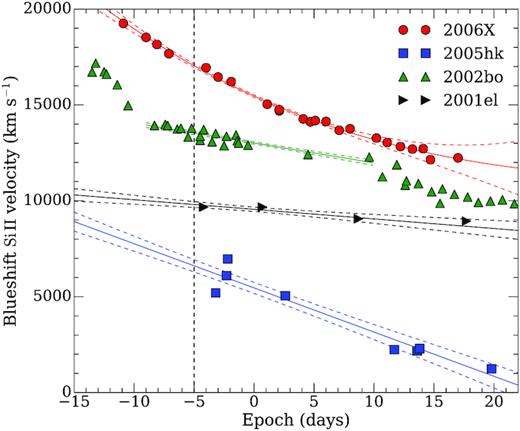
A third-order polynomial fit (solid lines), and the 1σ uncertainties (dashed lines) of the Si ii λ6355 Å velocities for SN 2005hk, SN 2002bo, SN 2001el, and SN 2006X. From the polynomial fits, we determined the velocity at −5 days relative to peak brightness (vertical black line). The individual velocity measurements are typically accurate within ∼75 km s−1 (the uncertainties are not depicted).
4.5 Measuring of the Si ii line polarization
Measuring the linear polarization of lines is challenging, because the peak polarization depends on the binning, and there are sometimes multiple peaks related to one absorption feature, e.g. the high-velocity and photospheric Si ii λ6355 Å line components (Wang et al. (Kasen et al. 2003; Wang et al. 2003; Branch et al. 2005; Mazzali et al. 2005; Silverman et al. 2015)
To measure the peak polarization of a specific line, we first manually determine the lower and upper wavelength edges containing the line of interest from a plot with all VLT flux and polarization spectra.
Finally, we measure the peak polarization value within the borders of the line. Fig. 7 shows the Si ii λ6355 Å line of SN 2002bo at −1 day relative to peak brightness, at three different bin sizes. Note that at this epoch, there are two peaks visible in the 25 and 50 Å binned spectra. The peaks correspond to the photospheric (with the lower velocity) and the high-velocity component of the Si ii λ6355 Å line. In this case, we measure the polarization of the higher peak. In the 100 Å binned data, the two peaks are blended.
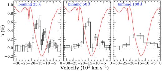
The linear polarization of the Si ii λ6355 Å line in SN 2002bo at −1 day relative to peak brightness. The three panels show the polarization degree derived with bin sizes of 25 Å (left), 50 Å (middle), and 100 Å (right). The error bars represent 1σ uncertainties. The grey line is the polarization spectrum not corrected for bias, and the red line is the flux spectrum of the Si ii line.
After the data reduction and the measurements, we can now investigate the evolution of the line polarization as a function of time. Fig. 8 shows the peak polarization of the Si ii λ6355 Å line in SN 2006X, as a function of time, for three different bin sizes of 25, 50, and 100 Å, compared to the measurements in Patat et al. (2009), who binned their data in ∼26 Å wide bins. This clearly shows that the measurements in highly binned data (100 Å) exhibit less variability, and have lower values, but when the polarization is measured in data with smaller bin sizes (25 and 50 Å), the measured peak polarization is higher, but so is the scatter. The choice of the appropriate bin size is a compromise between retaining spectral resolution and increasing the SNR. Broader bins increase the SNR per bin, but smoothen the polarization features. In our analysis, we select the bin size depending on the necessity, and keep them consistent throughout the analysis. For instance, to search for distinct peaks in the Si ii λ6355 Å line, we require a high spectral resolution and use data with a bin size of 25 Å; to study the q–u loops (Section 4.6), we use 50 Å, which is a good compromise between resolution and SNR; and to study different polarization relations, we use 100 Å in order to increase the SNR.
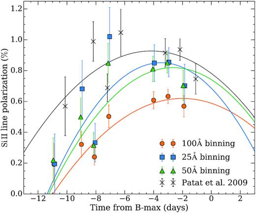
Peak polarization of the Si ii λ6355 Å line in SN 2006X, as a function of time, for three different bin sizes, compared to the measurements in Patat et al. (2009), who binned their data in ∼26 Å wide bins. The error bars represent 1σ uncertainties. Note that the time of peak brightness in Patat et al. (2009) is ∼1 day earlier than that used in this work.
A list of all peak polarization measurements of the Si ii λ6355 Å line, for different bin sizes, is given in Table A5 (Supporting Information) and plots of the line polarization and flux spectra of all SNe are presented in Appendix B (Supporting Information). Note that at later epochs (i.e. ≳25 days past peak brightness), the measured degrees of polarization around Si ii λ6355 Å are no longer representing the polarization of the Si ii feature, because at late epochs the absorption feature becomes increasingly contaminated by emerging lines from different ions (see Blondin et al. 2012).
To fit the Si ii polarization relations (e.g. in Fig. 8), we adopt the form |$p_{\rm Si\, \small {II}}$| = a × (t − tmax)2 + pmax, and use a nested sampling algorithm (Skilling 2004). We assume that the prior on the epoch of peak polarization, tmax, is a uniform distribution between −10 and 0 days, the prior on the peak polarization pmax variable is a uniform distribution between 0 and 5 per cent, and the prior on the parameter a is a uniform distribution between −1 and 0.
4.6 Analysis of the q–u loops
Depending on the geometry of the obscuring material, polarized lines sometimes display loops in the Stokes q–u plane (Section 2.2; see also Wang & Wheeler 2008). These loops result from variations of the polarization degree as a function of wavelength, i.e. velocity, and the polarization angle, due to non-axisymmetric distribution of the ejecta. The shape and orientation of the loops depend on the projected distribution of the absorbers in front of the photosphere (Kasen et al. 2003; Wang & Wheeler 2008; Branch & Wheeler 2017). Multi-epoch spectropolarimetry enables us to study the evolution of the 3D structure of the ejecta, and observe the change of the orientations of different chemical elements with epoch (see polar diagrams in Maund et al.(2009)). However, detailed analysis of individual SN Ia is out of the scope of this work, and in order to quantify the evolution of the loops in a systematic way, we will consider the loop area only, which preserves useful geometrical information about the scattering region.
Examples of loops are shown in Fig. 9. To analyse the loops, we use polarization values calculated with bins of 50 Å. We parametrize those loops by calculating the enclosed area within the loops. We first construct a convex hull from the (q, u) tuples. A convex hull of a set of points is the smallest convex set that contains the points (Barber, Dobkin & Huhdanpaa 1996). Examples of convex hulls, enclosing the loops, are shown in Fig. 9 (blue lines). Then, we calculate the area of the convex hull using the Shoelace algorithm (Braden 1986). The area of the loops is given in ‘units’ of (per cent)2, because it was determined in the q–u plane, with the values of q and u given in per cent. For instance, if the loop is a square with 1 per cent side, its area would be 1 (per cent)2. To estimate the error of the area, we run a Monte Carlo simulation by introducing a Gaussian error to the (q, u) tuples, 10 000 times for each epoch, and get a non-Gaussian distribution of the area values. We finally calculate the 25th and 75th percentiles of the distribution to estimate the semi-interquartile range.
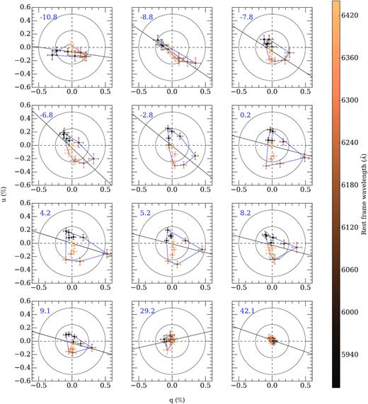
Evolution of the Si ii λ6355 Å line polarization in the q–u plane for SN 2005df. The bin size of the used data is 50 Å, and the wavelengths are colour coded. The error bars represent 1σ uncertainties. The panels show different epochs relative to peak brightness (indicated in the upper left corner of each insert). The blue lines trace the convex hull used to calculate the area, and the black lines trace the dominant axes computed using the displayed q, u data. The inner and outer concentric circles represent a polarization degree of 0.25 and 0.5 per cent, respectively.
5 RESULTS AND DISCUSSION
Line polarization has implications for the progenitor model and the explosion mechanism (Wang & Wheeler 2008; Bulla, Sim & Kromer 2015). The most prominent line polarization is observed in the Si ii λ6355 Å line and the near-IR Ca ii triplet (see Wang & Wheeler 2008). The maximum degree of polarization of the Si ii is typically ∼1 per cent, reached a few days before peak brightness. In this section, we show and discuss the evolution of the Si ii polarization, and the evolution of the loops in the q–u plane, discuss the Δm15–Si ii polarization relationship, investigate and interpret the Si ii velocity–polarization relationship, and finally compare our sample to simulations.
5.1 Time evolution of the Si ii polarization
Fig. 10 shows the time evolution of the peak polarization of the Si ii λ6355 Å line for a selected subset of SNe Ia, which are well sampled in terms of time coverage, measured with a binning of 100 Å. The evolution was discussed in Wang et al. (2007), who fit a time dependence for the degree of polarization with a second-order polynomial: |$p_{\rm Si\, \small {II}}$| = 0.65 − 0.041(t − 5) − 0.013(t + 5)2, where t is the time in days relative to the peak brightness in the B-band. However, as Porter et al. (2016) already noticed, many events are strikingly different in their behaviour compared to the polarization–epoch dependence given in Wang et al. (2007). There are different peak polarization values, at a range of different epochs. The Si ii peak polarization values range from ∼0.1 per cent (in the case of SN 2002fk and SN 2001el) to ∼0.6 per cent in the case of SN 2006X. SN 2004dt is an exception and has a peak Si ii polarization greater than ∼1.4 per cent. The epochs of the peak polarization values range from ∼10 days before peak brightness to the time of peak brightness.
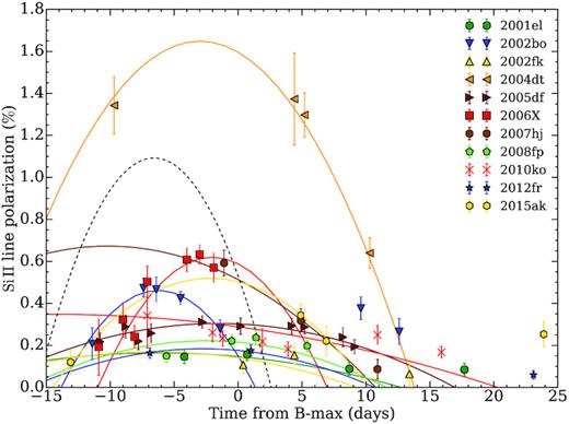
Time evolution of the peak polarization of the Si ii λ6355 Å line, for a sample of SNe Ia. For comparison, the dotted line shows the |$p_{\rm Si\, \small {II}}$|–epoch fit from Wang et al. (2007). Note that our polarization measurements are systematically lower compared to the time dependence deduced by Wang et al. (2007), because we use 100 Å bins. To fit the polarization relations, we adopt the form |$p_{\rm Si\, \small {II}}$| = a × (t − tmax)2 + pmax (see Section 4.5).
Inspecting the high-resolution polarization spectra, binned to 25 Å, we noticed that in some cases two distinct Si ii λ6355 Å peaks are visible. The two peaks correspond to a high-velocity and a lower velocity photospheric component of the Si ii line (Mazzali et al. 2005). These supernovae are listed in Table 2 (see also Appendix B in the Supporting Information). Both polarization peaks are prominent at the listed epochs in Table 2, although the two velocity components can often be identified also at other epochs.
SNe Ia with both high-velocity and photospheric Si ii λ6355 Å polarization peaks.
| Name | Epochs (relative to peak brightness) |
|---|---|
| SN 2002bo | −4.5, −1.4, and 9.6 days |
| SN 2002el | −7.6 days |
| SN 2003eh | 0.0 days |
| SN 2003W | All three epochs from −8.7 to 16.1 days |
| SN 2005df | 8 epochs from −10.8 and −5.2 days |
| SN 2005el | −2.7 days (the only observed epoch) |
| SN 2007fb | 6.0 days |
| SN 2007hj | 4.9 days |
| SN 2008fp | −0.5 and 1.4 days |
| SN 2010ev | −1.1 and 2.9 days |
| SN 2012fr | −6.9 and 1.0 days |
For the purpose of our statistical analysis, we always measure the highest peak of the Si ii λ6355 Å line (Section 4.5), except in the case of SN 2002bo and SN 2005df, which are well sampled (observed at 7 and 12 epochs, respectively) and display distinct high-velocity and photospheric components in the Si ii λ6355 Å polarization feature. Although it is beyond the scope of the paper to study individual objects in detail, for these two SNe we measured the polarization of the two velocity components separately with the aim of studying their evolution. To identify the polarization peaks that correspond to the two velocity components, we compared the polarization spectra at different epochs and manually selected the bins that correspond to the high-velocity and photospheric components, respectively, if they were visible. The time evolution of the high-velocity and photospheric Si ii λ6355 Å components for SN 2002bo and SN 2005df is presented in Fig. 11. In SN 2002bo, between epochs −1.4 and 9.6, the polarization of the photospheric component becomes (and stays) more prominent than the high-velocity component. The same behaviour is observed in SN 2007fb between epochs 3.0 and 6.0, as well as in the case of SN 2010ev between 2.9 and 11.9 days. On the other hand, in SN 2005df, the high-velocity component is more prominent only at the earliest observed epoch of −10.8 days and is relatively constant, while the photospheric component is more prominent between epochs of −10.8 and 9.1 days.
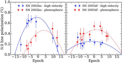
Time evolution of the peak polarization of the high-velocity (blue symbols) and photospheric (red symbols) Si ii λ6355 Å components, for SN 2002bo (left-hand panel) and SN 2005df (right-hand panel). The peak polarization of the two components was measured on polarization spectra with 25 Å bin size. To fit the polarization relations, we adopt the form |$p_{\rm Si\, \small {II}}$| = a × (t − tmax)2 + pmax (see Section 4.5).
We note that, although the velocity of the Si iiλ6355 Å absorption minima at peak brightness of SN 2002bo (|$v_{\rm Si\, \small {II}}$| = −12 854 ± 59 km s−1) is higher compared to the Si ii λ6355 Å absorption minima velocity of SN 2005df (|$v_{\rm Si\, \small {II}}$| = −9495 ± 37 km s−1), the velocities of the high-velocity polarization peaks of both SNe are comparable and consistent with the Si velocities of the ‘HV’ subclass of SNe Ia (vSi ≥ 12 000 km s−1; Wang et al. 2009). The velocities of the high-velocity polarization peaks of SN 2002bo and SN 2005df are approximately −14 × 103 and −15 × 103 km s−1, respectively.
5.2 |${\Delta } m_{15}\!-\!p_{\rm Si\, \small {II}}$| relationship
Wang et al. (2007) presented peak polarization measurements of the Si ii λ6355 Å line for a sample of 17 SNe Ia. They found a correlation between the degree of the peak polarization of the Si ii line and the light-curve decline rate, Δm15: |$p_{\rm Si\, \small {II}}$| = 0.48(03) + 1.33(15)(Δm15 − 1.1), where Δm15 is the decline in B-magnitude from peak brightness to the brightness 15 days after peak (Phillips 1993) and |$p_{\rm Si\, \small {II}}$| is in per cent. They argue that this trend provides strong support for DDT models, as the dimmer SNe, which burn less material to thermonuclear equilibrium, are expected to have larger chemical irregularities (thus larger polarization). This is due to the fact that more complete burning tends to erase chemically clumpy structures, and produces less chemically asymmetric explosions (see also Wang & Wheeler 2008).
As part of our analysis, we studied the Δm15–|$p_{\rm Si\, \small {II}}$| relationship using our larger sample and compared our Si ii polarization measurements to the literature. Fig. 12 shows peak linear polarization measurements of the Si ii λ6355 Å line, measured from 50 Å binned data, compared to the |$\Delta m_{15}\!-\!p_{\rm Si\, \small {II}}$| relationship determined by Wang et al. (2007) and measurements by other authors.
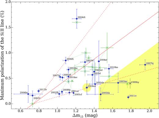
Peak polarization of the Si ii λ6355 Å line, measured at 50 Å binned data, between epochs −10 and 0, as a function of Δm15 (blue dots). The red full line is the |$\Delta m_{15}\!-\!p_{\rm Si\, \small {II}}$| relationship determined by Wang et al. (2007), and the red dashed lines indicate the 1σ level of the most likely distribution of polarizations from their Monte Carlo simulation. For comparison, we show measurements of the same SNe by other authors (green ’x’ symbols connected with dotted lines). SN 2006X, SN 2005hk, and SN 2005ke have been measured by Patat et al. (2009), Maund et al. (2010a), and Patat et al. (2012), respectively. All other green ’x’ symbols represent the measurements by Wang et al. (2007). The yellow area includes subluminous and transitional objects. For comparison, we additionally included the subluminous SN 1999by (black ’x’; Howell et al. 2001; Wang et al. 2007). Also note that SN 2004eo is classified as a transitional supernova.
Our linear polarization measurements of the Si ii line in SN 2002fk, SN 2001el, SN 2005cf, and SN 2004eo are systematically lower compared to the literature, independent of the binning size, whereas our measured Si ii polarization in SN 2004ef is lower in the case of the 100 Å binned data, and consistent with the literature in the case of 25 and 50 Å binned data. The SNe in the yellow region of Fig. 12 are subluminous and transitional objects. The 91bg-like SN 1999by (Howell et al. 2001), the 2002cx-like SN 2005hk (Maund et al. 2010a), and the 1991bg-like SN 2005ke (Patat et al. 2012) are well-known subluminous events. SN 2011iv is a transitional object (Gall et al. 2018) that has photometric and spectroscopic properties between a normal SN Ia and a subluminous 1991bg-like SN (see also Ashall et al. 2018; Mazzali et al. 2018). A near-maximum spectrum of SN 2007hj showed that it is similar to several subluminous SNe Ia, characterized by a strong Si ii absorption feature at 580 nm (Blondin et al. 2007). Blondin et al. (2012) classified SN 2007hj as CL (‘Cool’), which is characterized by deeper Si ii λ5972 Å absorption, often associated with low-luminosity objects. Furthermore, Pastorello et al. (2007) suggest that SN 2004eo should be considered as a transitional supernova, and Blondin et al. (2012) classified it as CL.
SN 2004dt has an exceptionally high peak polarization of the Si ii line (Wang et al. 2006). Predictions of polarization in the violent-merger scenario are in good agreement with such observations (Bulla et al. 2016a); however, the explosion scenario is still debated (see also Altavilla et al. 2007). In addition, SN 2003eh also shows high peak polarization of the Si ii line (∼0.8 per cent); however, it is not shown in Fig. 12, because the lack of photometric data prevented us from deriving the decline rate Δm15.
After removing the peculiar objects, the remaining data follow the |$\Delta m_{15}\!-\!p_{\rm Si\, \small {II}}$| relationship, although the scatter is larger than that for the measurements presented in Wang et al. (2007). The Pearson correlation coefficient for our sample, ρ = 0.63 (p-value = 0.005), is lower than the coefficient determined by Wang et al. (2007), ρ = 0.87. Note that in Fig. 12, we plot the maximum polarization within a range of −10 to 0 days relative to peak brightness, but we do not correct the polarization to a specific epoch (e.g. Wang et al. (,2007) corrected their observations to −5 days relative to peak brightness using a deduced time dependence of the degree of polarization), because, as discussed in the previous section, the polarization evolves in a variety of different ways and, despite the similarity of some polarization–epoch curves, we did not identify a common pattern that could be used to normalize all of them. Furthermore, we measured the peak polarization of the Si ii line using a constant bin size, while the binning used in Wang et al. (2007) is not given. They collected the peak polarization measurements of the Si ii line from the literature for a subsample of objects and combined them with their own measurements. Therefore, the bin size used for the measurements presumably differs from object to object.
The correlation between Δm15 and |$p_{\rm Si\, \small {II}}$| is not expected to be necessarily high, and the dispersion of the polarization may be a valuable diagnostic tool. Wang et al. (2007) used a toy model to constrain the number of clumps and the opacity of inhomogeneities based on the observed dispersion. Their model assumes that the clumps are randomly distributed above a spherical photosphere dominated by electron scattering. The size and number of clumps then determine the observable degree of polarization, which is also constrained by the depth of the Si ii absorption line profile. In such a model, the degree of polarization has a probability density distribution with a peak of about 0.5 per cent for 20 clumps covering the surface of the photosphere. Reducing the number of clumps introduces higher degrees of polarization and a larger dispersion of the degree of polarization. The results of their Monte Carlo simulation of this effect are shown in fig. 2 of Wang et al. (2007), and for comparison in Fig. 12. Our sample of normal SNe Ia is within the 1σ level of the most likely distribution of polarizations from their simulation. The large dispersion of the SNe may imply that there are a small number of large clumps (likely large-scale plumes or globally asymmetric chemical distributions) in the SN ejecta.
5.3 Si ii velocity–polarization relationship
Among the various possible correlations that we explored, we found a strong linear correlation between the degree of peak polarization and the expansion velocity of the Si ii λ6355 Å line. Fig. 13 shows a subset of our sample of SNe Ia that have at least one observation between −11.0 and 1.0 days relative to peak brightness. This selection produces a set of 23 SNe, observed within a relatively short range of time. The plot shows the maximum Si ii λ6355 Å polarization in that period, as a function of the Si ii λ6355 Å velocity at 5 days before peak brightness, vSi ii−5. The Si ii velocity has been determined from spectra (as described in Section 4.4) and the Si ii polarization degree was measured from spectra of 100 Å bin size (see Section 4.5).
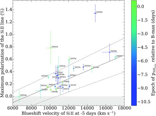
Maximum linear polarization of the Si ii λ6355 Å line between −11 and 1 days relative to peak brightness (measured on polarization spectra of 100 Å bin size), as a function of the Si ii λ6355 Å velocity at 5 days before peak brightness. The error bars represent 1σ uncertainties. The colours indicate the epoch of the peak Si ii λ6355 Å polarization relative to peak brightness. The black solid line is the linear least-squares fit to the data, and the dashed lines mark the 1σ uncertainty. Note that the relationship is not valid for velocities ≲7500 km s−1, because negative degrees of linear polarization are unphysical (grey area).
There are two clear outliers: SN 2004dt, which has been already studied by Wang et al. (2006) and may be the result of a violent merger (Bulla et al. 2016a), and SN 2003eh. There is no photometry available in the literature for this object; therefore, the Δm15 value for this supernova is not known. However, we found spectra taken at six epochs in the literature (see Table A3 in the Supporting Information), and obtained two spectropolarimetry observations at peak and 12 days past peak brightness. Therefore, the epoch of peak brightness has been estimated from spectra and has a large uncertainty of ±10 days. This object has been identified as a reddened SN Ia by Matheson et al. (2003). We confirm the classification using our VLT observations and the Supernova Identification (SNID) code (Blondin & Tonry 2007). The spectrum of SN 2003eh at peak brightness best matches the spectrum of SN 2008ar at 7 days past peak brightness. The total polarization spectra show a continuum, which rises from red to blue wavelengths, and highly polarized lines, similar to SN 2004dt. The continuum polarization reaches ∼1.5 per cent at 4000 Å, remains constant at both epochs, and is most likely produced by interstellar or circumstellar dust.
Linear regression test results for the |$p_{\rm Si\, \small {II}}$| versus Si ii velocity relationship. ‘No.’ is the number of included SNe in the epoch range (days relative to peak brightness). ρ and p-value are the Pearson correlation coefficient and the probability of an uncorrelated data set, respectively. α and β are the slope (in % mag−1) and the y-intercept (in %) of a linear least-squares fit, respectively.
| Epoch range | No. | ρ | p-value | α (×10−5) | β |
|---|---|---|---|---|---|
| −15.0 to 0.0 | 23 | 0.738 | 5.77 × 10⁻⁵ | 5.93 ± 1.38 | −0.436 ± 0.161 |
| −11.0 to 1.0 | 23 | 0.804 | 3.71 × 10⁻⁶ | 6.40 ± 1.28 | −0.484 ± 0.147 |
| −10.0 to 0.0 | 21 | 0.803 | 1.17 × 10⁻⁵ | 6.39 ± 1.37 | −0.483 ± 0.159 |
| −10.0 to −5.0 | 13 | 0.756 | 2.77 × 10⁻³ | 6.53 ± 2.16 | −0.536 ± 0.259 |
| −5.0 to 0.0 | 13 | 0.812 | 7.41 × 10⁻⁴ | 6.34 ± 1.40 | −0.453 ± 0.163 |
| 0.0–5.0 | 13 | 0.391 | 0.187 | 2.45 ± 2.00 | −0.091 ± 0.223 |
| 0.0–10.0 | 15 | 0.375 | 0.169 | 3.98 ± 2.09 | −0.275 ± 0.233 |
| 5.0–10.0 | 9 | 0.404 | 0.281 | 4.21 ± 3.80 | −0.313 ± 0.411 |
| 10.0–20.0 | 13 | 0.806 | 0.87 × 10⁻³ | 5.38 ± 1.35 | −0.440 ± 0.149 |
| 20.0–30.0 | 4 | 0.560 | 0.44 | 1.19 ± 3.90 | −0.054 ± 0.460 |
The interpretation of the velocity–polarization relation is not completely straightforward. In general, Fig. 13 connects the kinematics with ejecta asymmetry. If the relation is satisfactorily fit with one single linear function, it would imply that the geometric structure of the SNe is quite consistent and the differences in the polarization degree are caused largely by simple effects such as geometric projection towards the observer, or strong correlation between the observed ejecta velocity and absorption depth with ejecta asymmetry. If the dispersion of polarization across the fitted mean line of |$v_{\rm Si\, \small {II}}\!-\!p_{\rm Si\, \small {II}}$| is low, it might suggest that the number of lumps covering the photosphere is either very small or so large that effectively only a global asymmetry matters.
5.3.1 Off-centre DDT model
The velocity–polarization relationship may be explained in the context of a combination of an off-centre DDT model and brightness decline (Höflich et al. 2006). This can be understood with the following considerations. If for Chandrasekhar mass supernovae, for the range of normally bright to subluminous supernovae,4 the peak brightness depends on the amount of 56Ni produced in the explosion (Höflich et al. 2002, 2006), then intermediate mass elements (including silicon) are produced in larger quantities with decreasing peak brightness (i.e. increasing Δm15).
A reasonable scenario involves the dynamical structure of the ejecta. For example, in the context of DDT models, the Si ii line polarization is formed when the underlying Thomson photosphere is covered by Si-rich matter with high optical depth. Silicon and sulphur are produced in the quasi-statistical equilibrium group in oxygen burning, flanked by explosive carbon and elements produced in nuclear statistical equilibrium. Therefore, the Si polarization is formed after the photosphere passed the O/Ne/Mg–Si/S interface. For normal SNe Ia, this happens ∼7 to 5 days before peak brightness, while for subluminous supernovae the photosphere recedes faster in mass and the interface happens at higher density (Höflich et al. 2002).
If for a given SN Ia explosion the Si line polarization is formed further out (higher velocity) with less mass involved, the polarization may be higher. The reason is that off-centre delayed detonation in SNe Ia does not always occur at the same distance from the SN centre. Larger off-centre distances of DDT lead to more Si at high velocities (see Höflich et al. 2002, 2006). Furthermore, as discussed in Wang et al. (2007), higher silicon polarization values suggest that there are more compositional irregularities left in the central region by the pure deflagration phase, and thus less material is burned to thermonuclear equilibrium.
Fig. 14 shows SNe Ia in the |$\Delta m_{15}\!-\!v_{\rm Si\, \small {II}}$| plane. The colour-coded dots (depending on the Si ii polarization) are SNe in our VLT sample. The Si ii velocities correspond to the velocity at peak brightness.5 For comparison, we plot an additional sample of ∼100 SNe Ia from the Open Supernova Catalog (grey dots; Guillochon et al. 2017) that includes well-observed SNe Ia with spectra close to day 0 and a sufficient number of photometric measurements. We fit their light curves with SNooPy and determine Δm15 as described in Section 4.3, and measure the Si ii velocity as explained in Section 4.4. SNe with normal Si ii velocities (∼9000–12 000 km s−1) are distributed across the whole range of Δm15 values, while the SNe with high silicon velocities (≳12 000 km s−1) are clustered around Δm15 ∼ 1.1 mag (Fig. 14). This can be explained as a consequence of an asymmetric DDT scenario. Models show that, for a given Δm15, the asymmetric detonation pushes Si out aspherically (predominantly in one direction), and line polarization produced by Si starts to form in the regions with higher velocities. For example, at day −5 in normal and subluminous SNe we observe line polarization produced by the outermost material only, and not the entire ejected Si material (see off-centre DDT models in Fesen (,2004) and Höflich et al. (2006), and chemical structures in Höflich et al. (2002)). This is the high-velocity end in the |$\Delta m_{15}\!-\!v_{\rm Si\, \small {II}}$| relation. Furthermore, it is expected that the Si ii velocity increases with decreasing Δm15 (see Höflich et al. 2002).
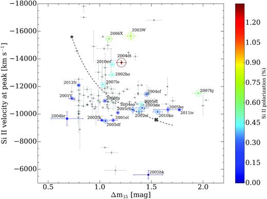
Supernovae Ia in the |$\Delta m_{15}\!-\!v_{\rm Si\, \small {II}}$| plane. The Si ii velocity corresponds to the velocity at peak brightness. The coloured dots represent the VLT sample. The colour of the dots and circles indicates the maximum polarization degree of the Si ii λ6355 Å line measured between −11 and 1 days relative to peak brightness, on polarization spectra of 100 Å bin size. The radius of the circles is proportional to the polarization degree. The dashed line corresponds to numerical predictions for sub-Chandrasekhar white dwarfs with masses from 0.9 M⊙ (⋆) to 1.2 M⊙ (×), and a thin 0.01 M⊙ He shell (Polin et al. 2019). A sample of archival SNe Ia (grey dots) from The Open Supernova Catalog is shown for comparison.
5.3.2 DDET model
Although the off-centre DDT explosion scenario provides a good explanation of the observations, a DDET scenario cannot be excluded. Polin, Nugent & Kasen (2019) perform an analysis of the numerical parameter space of 1D sub-Chandrasekhar mass white dwarf explosion models and found a correlation between mass, brightness, and the Si ii velocity exhibited in these DDET models with thin helium shells. Polin et al. (2019) predicted the Si ii line velocity as a function of the absolute peak brightness in B-band, M|$\rm _B$|, for sub-Chandrasekhar white dwarfs with a thin 0.01 M⊙ He shell and a range of white dwarf masses (see fig. 11 in Polin et al. 2019). In Fig. 14, we included these numerical predictions6 (dashed line; Polin et al. 2019). The dashed line traces the |$\Delta m_{15}\!-\! v_{\rm Si\, \small {II}}$| predictions for different white dwarf masses: from 0.9 M⊙ at the faint end (i.e. large Δm15 values) to 1.2 M⊙ at the bright end (see fig. 11 in Polin et al. 2019).
Polin et al. (2019) compared their numerical predictions to a sample of well-observed SNe (Zheng, Kelly & Filippenko 2018) and found evidence of two distinct populations in the Si ii velocity–M|$\rm _B$| plane, having masses close to either the Chandrasekhar or sub-Chandrasekhar masses. Fig. 15(a) shows a direct comparison between the Zheng et al. (2018), the Open Supernova Catalog, and our VLT sample in the |$\Delta m_{15} \!-\! v_{\rm Si\, \small {II}}$| plane. The blue ellipse denotes the cluster of SNe that are suggested to be exploding Chandrasekhar mass white dwarfs, and the other SNe that fall uniformly above the numerical predictions are suggested to be sub-Chandrasekhar mass white dwarfs (Polin et al. 2019). The three samples coincide with each other, except that our sample from the Open Supernova Catalog includes a broader brightness range of supernovae, from normal to subluminous supernovae. Therefore, the two possible populations of SNe do not appear as distinct in the Open Supernova Catalog sample (grey dots), as they do in the Zheng et al. (2018) sample (black dots).
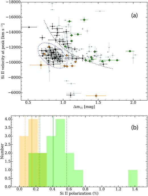
(a) SNe Ia in the |$\Delta m_{15}\!-\!v_{\rm Si\, \small {II}}$| plane. The orange and green diamonds represent the VLT sample, which is divided into Chandrasekhar-like (orange diamonds) and sub-Chandrasekhar SNe (green diamonds). The sample from Zheng et al. (2018) (black dots) is consistent with the sample from the Open Supernova Catalog (grey dots). The dashed blue ellipse marks the ‘cluster’ of Chandrasekhar-like SNe, which may be a distinct population of SNe Ia, relative to the sub-Chandrasekhar SNe that are located along the numerical predictions for sub-Chandrasekhar white dwarfs with a thin He shell (grey dashed line; Polin et al. 2019). (b) Distribution of the peak polarization of the Si ii line for the VLT sample in part (a) located above the |$\Delta m_{15} \!-\! v_{\rm Si\, \small {II}}$| prediction of Polin et al. (2019) (green colour), compared to the subsample in the ‘cluster’ (orange colour), under the numerical prediction. The average polarization of the SNe in the cluster is |$p_{\rm Si\, \small {II}}$| = 0.15 ± 0.08 per cent, and the average polarization of the SNe above the |$\Delta m_{15} \!-\! v_{\rm Si\, \small {II}}$| prediction is |$p_{\rm Si\, \small {II}}$| = 0.41 ± 0.16 per cent (after excluding SN 2004dt).
We note that neither of the samples perfectly traces the |$\Delta m_{15}\!-\! v_{\rm Si\, \small {II}}$| numerical prediction. However, following Polin et al. (2019) we grouped supernovae into the ‘cluster’ of objects that have a normal peak brightness and normal Si ii velocities (orange diamonds in Fig. 15a) and those that are suggested to be sub-Chandrasekhar mass white dwarfs (and fall above the prediction, green diamonds). Interestingly, the supernovae with higher polarization of the Si ii line tend to lie above the numerical |$\Delta m_{15}\!-\! v_{\rm Si\, \small {II}}$| predictions for sub-Chandrasekhar mass explosions by Polin et al. (2019), compared to supernovae in the ‘cluster’, below the |$\Delta m_{15}\!-\! v_{\rm Si\, \small {II}}$| line (Fig. 15a), that have lower polarization degrees of the Si ii line. In Fig. 15(b), we show the Si ii line polarization distribution for SNe of the two distinct groups. The average polarization of the SNe in the ‘cluster’ is |$p_{\rm Si\, \small {II}}$| = 0.15 ± 0.08 per cent, and the average polarization of the sub-Chandrasekhar mass SNe is |$p_{\rm Si\, \small {II}}$| = 0.41 ± 0.16 per cent (after excluding SN 2004dt).
5.3.3 Other models
Alternatively, the large-scale asymmetry of the Si ii line formation region as inferred from this data set may also be explained in the context of merging scenarios. It is not clear how this large-scale asymmetry above the Si ii layer is related to the rather spherical photosphere post-optical maximum. Bulla et al. (2016a) investigated polarization signatures for the violent-merger model by Pakmor et al. (2012). Bulla et al. (2016a) could not reproduce the low levels of Si ii line polarization typically observed in normal SNe Ia. However, the ejecta morphologies for other merger scenarios, e.g. the tidal mergers involving an accretion phase (e.g. Benz et al. 1990) or violent head-on collisions (e.g. Rosswog et al. 2009; see also Livio & Mazzali 2018, for summary of merger scenarios), may produce different polarization signatures. These data provide new observational diagnostics for more theoretical understandings of SN Ia physics.
5.4 Si iiq–u loops
Some SNe included in our sample draw loops in the q–u plane in the wavelength range around the Si ii λ6355 Å line (see Appendix B in the Supporting Information). These SNe are listed in Table 4. Other SNe may show a loop on at least one epoch, but they are below the noise level and cannot be analysed in a statistically meaningful way.
SNe Ia with loops in the q–u plane in the wavelength range around the Si ii λ6355 Å line.
| Name | Epochs (relative to peak brightness) |
|---|---|
| SN 2005df | 8 epochs from −7.8 to 9.1 days |
| SN 2006X | 5 epochs from −8.1 to −1.9 days |
| SN 2002bo | 5 epochs from −7.4 to 9.6 days |
| SN 2004dt | 4 epochs from 4.4 to 33.2 days |
| SN 2007fb | 3 and 6 days |
| SN 2010ko | 1.9 and 10.9 days |
| SN 2015ak | Clear loop at 4.9 days |
| SN 2010ev | 11.9 days |
| SN 2011ae | 4 days |
| SN 2007hj | −1.1 days |
| SN 2005ke | −9.1 days |
| SN 2005cf | −5.8 days |
| SN 2001el | Clear but small loops at −4.2 and 0.7 days |
To characterize in a quantitative way the evolution of the loops, we calculated the area inside of the loops, using polarization spectra binned to 50 Å, as described in Section 4.6. Fig. 16 shows the area, A, as a function of epoch, for a subsample of SNe observed on at least four epochs before 30 days past peak brightness. The largest loops were observed in SN 2006X, SN 2002bo, and SN 2005df. The area of the loops in these SNe smoothly evolves and is largest between approximately −5 and ∼5 days relative to the peak brightness. The peculiar SN 2004dt is located outside of the axis limits (A > 0.32 (per cent)2, up to A ∼ 1.75 (per cent)2 at 4.4 days past peak).
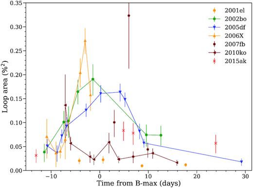
The area contained in q–u loops as a function of epoch. Shown are all SNe that have been observed on at least four epochs (SN 2004dt is off scale in area). The lines connect measurements of SNe that have been observed on five epochs or more. The error bars represent the semi-interquartile range.
To explore the effect of clumps on the polarization spectra and q–u plane, we run simple simulations (see Bulla 2017, for more details). In the simulations, we make the following assumptions:
spherical ejecta;
photosphere at 10 000 km s−1;
roughly 0.5 M⊙ above the photosphere;
outer boundary: vouter ∼ 20 000 km s−1;
density power-law index = 7;
density at the photosphere = 7 × 10⁻¹⁴ g cm−3;
electron scattering optical depth: τes ∼ 0.6;
line opacity outside clumps: τline = 1;
line opacity inside clumps: τline clumps = 10.
The clump positions are randomly generated in regions of the ejecta moving towards the observer (blueshifted velocities). The signs of q and u are defined as in Bulla et al. (2015). Also, the clump centres are randomly generated between the inner (photosphere) and outer boundary. Depending on the sizes, some regions of the clumps could actually fall either inside the photosphere or outside the ejecta (see upper panels in Fig. 17).
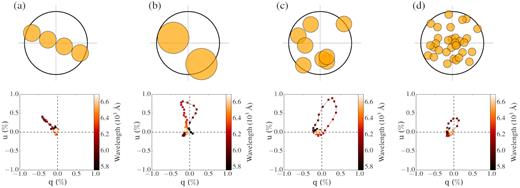
Simulations of polarization induced by clumps, for four different scenarios. The upper panels illustrate the size and distribution of clumps (filled orange circles) in front of the photosphere (large circle), while the bottom panels show the resulting polarization in the q–u plane. Panel (a) shows four clumps axisymmetrically distributed. It produces polarization, but no loops in the q–u plane. The other three panels (b–d) illustrate randomly distributed clumps of different sizes. The smallest clumps produce a small loop, compared to the clumps of intermediate and large size.
Fig. 17 shows simulations for four different scenarios. The left-hand panel presents the case of four clumps with an axisymmetric distribution, to simulate the effect of a torus-like geometry. The clump sizes (in velocity space) are vouter/4.0 = 5000 km s−1. The other three panels show randomly distributed clumps, from left to right: 2 clumps with radius vouter/2 = 10 000 km s−1, 8 clumps with radius vouter/4 = 5000 km s−1, and 32 clumps with radius vouter/8 = 2500 km s−1. The total covering factor of the clumps would be equal in the three simulations if there was no overlapping. Non-zero polarization levels across the spectral line are found for all four scenarios. In the case of an axisymmetric distribution of the clumps, there are no loops in the q–u plane, while for non-axisymmetric distributions, loops are produced. The loop areas are similar for the first two distributions, but smaller in the third case with small clumps.
Previous studies already suggested that the Si ii line polarization is produced by large clumps, i.e. large-scale asymmetry. Maund et al. (2010b) report that the velocity evolution of the Si ii λ6355 Å line, v̇|$\rm _{\rm Si\, \small {II}}$|, is linearly related to the polarization of Si ii. They suggest that the velocity evolution is predominantly due to a general asymmetry and that the Si ii polarization is unlikely to be produced by small randomly distributed clumps, but rather by a general asymmetry of the ejecta. Furthermore, Wang et al. (2007) also suggest that the |$\Delta m_{15}\!-\! p_{\rm Si\, \small {II}}$| relation is an indication of a large-scale asymmetry, for instance, in form of large clumps above the photosphere in the outermost layers.
However, in this section we study the evolution of the Si ii polarization in the q–u plane and demonstrate the importance of high-cadence spectropolarimetric observations, which enables us to study the evolution of the ejected material and reveals a non-monotonic and complex behaviour with time. In SN 2005df, SN 2006X, and SN 2002bo, which have been observed at many epochs, we can observe the evolution of the polarization of the Si ii line, from high polarization and no loops, over large loops, to small loops (see all plots in Appendix B in the Supporting Information). By comparing to the simple simulations in Fig. 17, the evolution of loops can be explained by the change of the silicon ejecta geometry and clump size, from large axisymmetric structures, to large clumps, and finally to small clumps, as time evolves and the photosphere moves inwards.
We notice that in SN 2002bo and SN 2005df, which also display the Si ii photospheric and high-velocity components in the polarization spectra, the individual velocity components also display distinct q–u loops at some epochs. In Fig. 18, the polarization of the photospheric and high-velocity components is connected with the orange (dotted) and the blue (solid) line, respectively. Although the data at high resolution (with bin size of 25 Å) have large uncertainties, and are not of sufficient quality to study the time evolution of the distinct loops, these are visible in the case of SN 2002bo, which has both prominent photospheric and high-velocity components, in contrast to SN 2005df that displays prominent photospheric lines (and its corresponding loop), but has a relatively low polarized high-velocity component (see Fig. 10), and therefore displays a small loop at 0.2 days past peak brightness.
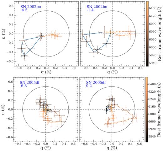
Polarization of the Si ii λ6355 Å line in the q–u plane for SN 2002bo (upper panels) and SN 2005df (bottom panels) at two selected epochs. The colour of the dots indicates the wavelength. The orange (dotted) and blue (solid) lines connect the dots that correspond to the photospheric and high-velocity components, respectively. The circle represents a polarization degree of 0.5 per cent.
5.5 Comparison to simulations
We compared our sample to simulations by Bulla et al. (2016a,b), who computed polarization spectra for different SN Ia explosion models. In particular, we examined the silicon line velocities and the Si ii polarization in the polarization spectra of the DDT (Seitenzahl et al. 2013), DDET (Fink et al. 2010), and violent-merger (Pakmor et al. 2012) models, at −5, −2.5, 0, 2.5, 5, and 7.5 days relative to B-band maximum. We determined the maximum Si ii polarization and the wavelength of the absorption minimum to determine the photospheric expansion velocity. These values are calculated for different viewing angles in each model. Specifically, we use only viewing angles for which high signal-to-noise calculations are available: five orientations for DDT and violent-merger models and three orientations for the DDET model. The choices of these angles are explained in Bulla et al. (2016a,b), and given in Table A8 (Supporting Information), along with the measurements from the simulations of the Si ii velocities and polarization values.
The wavelength bin size in the simulated polarization spectra changes depending on the wavelength. Around the silicon line, the size of one pixel is ∼10 Å, but the polarization spectra were Savitzky–Golay filtered using a first-order polynomial and a window of 3 pixels (∼30 Å). Therefore, we compare our data that were measured on polarization spectra of 25 Å bin size to the simulations.
Fig. 19 compares our observations to the DDT, violent-merger, and DDET models. The simulations show that the polarization degree of the Si ii line in the violent-merger observations is higher compared to the DDT and DDET models. Furthermore, the DDT and DDET models have a comparable degree of polarization. Our observations of the peak polarization of the Si ii line are consistent with predictions for the DDT and DDET models, while only SN 2004dt has a comparable polarization to the predictions for the violent-merger model.
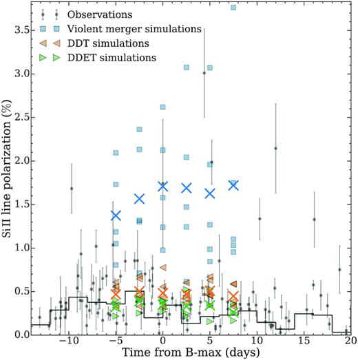
Observed peak polarization of the Si ii λ6355 Å line for all epochs (black dots, measured on polarization spectra of 25 Å bin size), compared to predictions by Bulla et al. (2016a,b) for the DDT (orange triangles pointing left), violent-merger (blue squares), and DDET (green triangles pointing right) models. Simulated values for multiple orientations at −5, −2.5, 0, 2.5, 5, and 7.5 days relative to B-max are shown. The crosses mark the values averaged over all orientations, and the full black line is the weighted mean of our observations.
The ejecta in the DDT model is globally distributed spherically symmetrical, and therefore, the degree of polarization is similar regardless of the viewing direction. On the contrary, in the violent-merger model, the higher polarization values typically correspond to viewing angles closer to the poles (away from the equatorial plane; see Table A8 in the Supporting Information). The DDET model is symmetric about the z-axis, and therefore, three orientations were sufficient to properly sample this model. For the DDET model, the viewing angles closer to the equatorial plane typically display slightly higher polarization values, although the values are similar regardless of the viewing angle (Table A8, Supporting Information).
Fig. 20 shows the comparison between simulations and observations of the observed maximum polarization of the Si ii line between −11 and 1 days relative to peak brightness, against the Si ii velocity at 5 days before the peak brightness. The DDT and DDET simulations results coincide with the observations, and the degree of Si ii polarization in the violent-merger simulation is offset from the DDT and DDET simulations. Although the observations display a velocity–polarization trend, the velocity range of the simulations is not sufficient to reliably confirm a relationship. Note that the polarization of the Si ii line in this figure was measured on polarization spectra of 25 Å bin size, compared to Fig. 13, which shows the velocity–polarization relationship using polarization measurements on spectra with bin size of 100 Å.
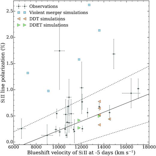
The observed maximum polarization of the Si ii λ6355 Å line between −11 and 1 days relative to peak brightness (black dots, measured on polarization spectra of 25 Å bin size), versus the Si ii velocity at 5 days before the peak brightness, compared to simulations. Red triangles pointing left mark the DDT model, blue squares the violent-merger model, and green triangles pointing right the DDET model. The lines show the observed velocity–polarization relationship (solid line) and the 1σ uncertainty (dashed line).
5.6 Intrinsic continuum polarization
Although the analysis of this paper is based on continuum-subtracted spectra (which implicitly removes the problem of ISP correction for the continuum polarization), our sample includes a number of objects affected by low or negligible reddening. This allows us to derive an upper limit on the intrinsic continuum polarization.
For this purpose, we determined the average continuum polarization from total polarization spectra with a bin size of 100 Å. The average continuum polarization was calculated in a region between 6400 and 7200 Å, which contains no strong spectral features (see section 5.4 in Patat et al. 2009). The results are given in Table A6 (Supporting Information).
Then, we estimated the reddening, E(B − V), by fitting the SN light curves from the Open Supernova Catalog with SNooPy (see Section 4.3), or took the E(B − V) values from the literature. The E(B − V) values with references are given in Table A7 (Supporting Information).
In the left-hand panel in Fig. 21, we show the maximum continuum polarization for each SN, measured before +15 days relative to peak brightness, as a function of reddening determined by fitting the SN light curves, E(B − V)fit. Although the best-fitting B − V colour of some SNe is bluer (approximately −0.1 mag) compared to normal SN Ia templates, possibly because of errors in the photometric data or intrinsic differences, there is always some amount of Galactic dust present, which can produce a polarization of up to 9 × E(B − V) per cent (hereafter, upper ISP limit; Serkowski et al. 1975), and should not be neglected. Therefore, we extracted the Galactic dust reddening values for all SN locations from Schlafly & Finkbeiner (2011) and compared the E(B − V)MW values to the reddening determined from the light curves of SNe, E(B − V)fit. In the right-hand panel in Fig. 21, we present the continuum polarization as a function of the larger reddening value, E(B − V)max = max[E(B − V)MW, E(B − V)fit]. This moves the blue SNe closer to the upper polarization limit, where the continuum polarization may be explained by ISM. A few SNe have a higher polarization compared to the ISP limit, which may be an indication of intrinsic SN continuum polarization; however, the confidence interval of the ISP upper limit is not given in the literature, and there are also some stars in the sample of Serkowski et al. (1975) that lie above the ISP limit. Another possible explanation why some SNe Ia lie above the ISP limit is a contribution of host galaxy dust to the observed polarization, and perhaps with a different polarization law (e.g. Leonard et al. 2002; Porter et al. 2016). Although the SNe Ia appear unreddened, the contribution of host galaxy dust cannot be excluded, as in the case of Galactic dust, which in contrast to the host galaxy dust was independently measured by Schlafly & Finkbeiner (2011). On the contrary, note that polarization by dust in the host galaxy could also partially cancel out polarization by Galactic dust, depending on the relative position angles.
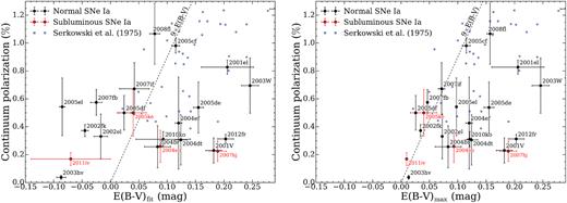
Continuum polarization as a function of E(B − V). The black and red dots depict normal SNe and subluminous/transitional SNe from our VLT sample, respectively. Milky Way stars from Serkowski et al. (1975) are included for comparison (grey squares). The dashed line marks the nominal upper ISP limit, 9 × E(B − V), determined from Milky Way stars (Serkowski et al. 1975). Left: The maximum continuum polarization for each SN, measured before +15 days relative to peak brightness, as a function of E(B − V)fit determined by fitting the SN light curves. Right: Same as the left-hand panel, but instead of E(B − V)fit, we use the larger reddening value of E(B − V)MW and E(B − V)fit. A few SNe Ia have a higher polarization compared to the nominal upper ISP limit, which may be an indication of intrinsic SN continuum polarization, or can be due to potential ISP contribution from the host galaxy (see discussion in Section 5.6).
Finally, to constrain the upper limit on the intrinsic continuum polarization of SNe Ia, we select a subsample of six SNe with E(B − V)max < 0.05 mag: SN 2002fk, SN 2003hv, SN 2005df, SN 2005ke, SN 2007fb, and SN 20011iv. The mean continuum polarization of these six SNe with low reddening is 0.32 ± 0.15 per cent. The upper limit is 0.61 per cent, with a confidence interval of 95 per cent. These results are consistent with the literature (Howell et al. 2001; Chornock & Filippenko 2008; see also item (iii) in Section 2.1 ). Assuming that there is no contribution from the ISP, and that the intrinsic continuum polarization is produced by electron scattering in an aspherical photosphere, the upper limit of intrinsic polarization of 0.61 per cent corresponds to an oblate ellipsoid with an axial ratio of E = a/b ≈ 0.88 seen at an inclination angle of 90° (see fig. 4 in Höflich 1991).
6 SUMMARY AND CONCLUSIONS
We reduced and examined, in a systematic way, archival linear spectropolarimetric data of a sample of 35 SNe Ia observed with the VLT’s FORS1 + FORS2 between 2001 and 2015 at 127 epochs in total. To the best of our knowledge, this is the largest polarimetric data set of SNe Ia ever examined. Our main results can be summarized as follows:
The peak polarization of the Si ii λ6355 Å line displays an evolution in time with a range of peak polarization degree from ∼0.1 to 1.7 per cent at epochs from −10 to 0 days relative to peak brightness (Fig. 10). This differs from previous studies based on smaller samples (Wang et al. 2007). Also, the polarization peaks of the distinct Si ii λ6355 Å velocity components behave differently (Fig. 11).
We populated the |$\Delta m_{15}\!-\! p_{\rm Si\, \small {II}}$| plane, and re-analysed the |$\Delta m_{15}\!-\! p_{\rm Si\, \small {II}}$| relationship proposed by Wang et al. (2007). Although the overall behaviour is reproduced, our larger sample reveals a significantly larger scatter. We show that subluminous and transitional objects display lower Si ii line polarization values and are located below the main |$\Delta m_{15}\!-\! p_{\rm Si\, \small {II}}$| relationship (Fig. 12). This confirms previous results based on smaller samples (Howell et al. 2001; Patat et al. 2012).
We found a statistically significant linear relationship (ρ ≳ 0.8) between the degree of linear polarization of the Si ii λ6355 Å line before maximum with the Si ii λ6355 Å line velocity (Fig. 13). We suggest that this relationship, along with the |$\Delta m_{15}\!-\! p_{\rm Si\, \small {II}}$| relationship (Wang et al. 2007), may be explained with the off-centre DDT model (Höflich et al. 2006).
However, a comparison of our sample in the Δm15–|$v_{\rm Si\, \small {II}}$| plane to numerical predictions for DDET explosions (Polin et al. 2019) revealed that there are two distinct subgroups. The SNe that fall uniformly above the sub-Chandrasekhar DDET explosion model prediction line display higher polarization degrees of the Si ii line compared to a distinct ‘cluster’ of normal Chandrasekhar-like SNe (see Figs 14 and 15). This dichotomy in the polarization may imply that there are indeed two distinct populations of SNe Ia, as suggested in Polin et al. (2019), with different explosion mechanisms. However, this tentative conclusion requires further theoretical investigations.
We examined the evolution of the Si ii line in the q–u plane for a subsample of SNe, observed at multiple epochs, and ran simple simulations to explore the effect of clumps on the polarization spectra. In the cases of SN 2005df, SN 2006X, and SN 2002bo, we observe the evolution of the formation of loops, their growth, and subsequent shrinking (see all plots in Appendix B in the Supporting Information), which may be explained by the evolution of the projected silicon ejecta size, from large axisymmetric structures to large clumps, and finally to small clumps as time evolves and the photosphere moves inwards.
We compared our sample of the Si ii polarization measurements to predictions calculated for the DDET, DDT, and violent-merger models by Bulla et al. (2016a,b). Our observations of the peak polarization of the Si ii line are consistent with predictions for the DDT and DDET models, which have a comparable degree of polarization. Only SN 2004dt has a degree of polarization that is comparable to predictions for the violent-merger model.
We attempted to reproduce the Si ii–velocity relationship using simulations by Bulla et al. (2016a,b). Although the calculations show a global velocity–polarization trend, the velocity range of the models available is not sufficient to stringently test the observed relationship.
Additionally, we determined an upper limit of the intrinsic continuum polarization. For a subsample of six objects with E(B − V) < 0.05 mag, we estimate an upper limit of 0.61 per cent, with a confidence of 95 per cent. This result is consistent with the literature. Assuming that the polarization is produced due to electron scattering in an aspherical photosphere, and that there is no contribution from ISP, this degree of polarization corresponds to an oblate ellipsoid with an axial ratio of a/b ≳0.88 seen at i = 90° (Höflich 1991).
This work shows that even typical SNe Ia display a distribution of polarization properties that illustrates a richness in the geometry of the explosion that is a challenge to models and that cannot be revealed by total flux spectra. The evolution of the Si polarization amplitude and the size of loops in the q–u plane suggest that the Si distribution gets more complex, ‘clumpier,’ with depth. If this structure is the result of plumes resulting from the burning dynamics, the plumes have a fine structure at greater depth but merge to a few large features in outer layers. Again, the implied Si plume structure is a new constraint on multidimensional models that is not revealed in total flux spectra. Furthermore, this work shows the power of increasing the sample size of SN with high-cadence spectropolarimetry. Only frequent observations enable the study of the evolution of the polarization of individual lines. Here, we have concentrated on the Si ii line, but a similar analysis should be done on other prominent lines. If the next generation of large ground-based telescopes is designed and build to support precision polarimetry, they will allow the study of the polarimetric evolution of different species, different velocity components (high velocity and photospheric), and q–u loops with high accuracy. This will allow us to reconstruct the 3D structure of the explosion and to study the polarimetric tomography in great detail. It is critical that the new generation of large telescopes has the capacity to do spectropolarimetry.
SUPPORTING INFORMATION
Table A1. Observing log.
Table A2. SN Ia light curves from the Open Supernova Catalog.
Table A3. SN Ia spectra from the Open Supernova Catalog.
Table A4. Si ii λ6355 Å blueshift velocity at −5 days relative to peak brightness.
Table A5. Si ii line polarization measured from polarization spectra with different bin sizes.
Table A6. Average continuum polarization measured from 6400 to 7200 Å.
Table A7. Reddening determined from SN light curves and Galactic reddening taken from Schlafly & Finkbeiner (2011).
Table A8. Measurements of the Si ii λ6355 Å line velocities and polarization values from simulations of the DDT, DDET, and violent-merger models (Bulla et al. 2016a,b).
Figures B1–B35. For all SNe: polarization of the Si ii λ6355 Å line at different epochs relative to peak brightness, and Si ii polarization in the q–u plane.
Figures C1-C127. Individual polarization spectra for all epochs.
Please note: Oxford University Press is not responsible for the content or functionality of any supporting materials supplied by the authors. Any queries (other than missing material) should be directed to the corresponding author for the article.
ACKNOWLEDGEMENTS
We would like to thank Jason Spyromilio, Thiem Hoang, Ivo Seitenzahl, Ashley Ruiter, Wolfgang Kerzendorf, Stefan Taubenberger, and Barna Barnabás for helpful discussions. A. Clocchiatti was supported by grant IC120009 (MAS) funded by the Chilean Ministry of Economy, Development and Tourism, and by grant Basal CATA PFB 06/09 from CONICYT. LW was supported by NSF 1817099. JCW was supported by NSF Grant 1813825. The research of YY was supported through a Benoziyo Prize Post-doctoral Fellowship. This work was based on observations collected at the European Organisation for Astronomical Research in the Southern Hemisphere under ESO programmes 67.D-0517(A), 66.D-0328(A), 68.D-0571(A), 69.D-0438(A), 70.D-0111(A), 71.D-0141(A), 073.D-0771(A), 073.D-0565(A), 075.D-0628(A), 075.D-0213(A), 076.D-0178(A), 076.D-0177(A), 079.D-0090(A), 080.D-0108(A), 081.D-0557(A), 081.D-0558(A), 085.D-0731(A), 086.D-0262(A), 086.D-0262(B), 088.D-0502(A), 095.D-0848(A), 095.D-0848(B), 290.D−5009(A), 290.D−5009(B), 290.D−5009(C), and 290.D−5009(D); the execution in service mode of these observations by the VLT operations staff is gratefully acknowledged.
This work benefited from The Open Supernova Catalog (http://sne.spac; Guillochon et al. 2017), SNooPy (Burns et al. 2011), SNID (Blondin & Tonry 2007), L.A.Cosmic (van Dokkum 2001), IRAF (Tody 1986), PyRAF, and PyFITS. PyRAF and PyFITS are products of the Space Telescope Science Institute, which is operated by AURA for NASA. We thank the authors for making their tools and services publicly available.
Footnotes
Note that this statement is strongly debated; e.g. Goldstein & Kasen (2018) suggest that only sub-Chandrasekhar mass explosions can reproduce the fast decline rates Δm15 > 1.55, while all SN Ia models (Chandrasekhar, sub-Chandrasekhar, and some super-Chandrasekhar mass white dwarf explosions) can reproduce the slow decline rates, 0.8 < Δm15 < 1.55.
We decided to plot the Si ii velocity at peak brightness instead of the velocity at 5 days before peak brightness, in order to be consistent with other works (see discussion later).
