


ABSTRACT
Observations of both gamma-ray bursts (GRBs) and active galactic nuclei (AGNs) point to the idea that some relativistic jets are suffocated by their environment before we observe them. In these ‘choked’ jets, all the jet’s kinetic energy is transferred into a hot and narrow cocoon of near-uniform pressure. We consider the evolution of an elongated, axisymmetric cocoon formed by a choked jet as it expands into a cold power-law ambient medium ρ ∝ R−α, in the case where the shock is decelerating (α < 3). The evolution proceeds in three stages, with two breaks in behaviour: the first occurs once the outflow has doubled its initial width, and the second once it has doubled its initial height. Using the Kompaneets approximation, we derive analytical formulae for the shape of the cocoon shock, and obtain approximate expressions for the height and width of the outflow versus time in each of the three dynamical regimes. The asymptotic behaviour is different for shallow (|$\alpha \leq 2$|) and steep (2 < α < 3) density profiles. Comparing the analytical model to numerical simulations, we find agreement to within ∼15 per cent out to 45 deg from the axis, but discrepancies of a factor of 2–3 near the equator. The shape of the cocoon shock can be measured directly in AGNs, and is also expected to affect the early light from failed GRB jets. Observational constraints on the shock geometry provide a useful diagnostic of the jet properties, even long after jet activity ceases.
1 INTRODUCTION
Relativistic jets are ubiquitous in high-energy astrophysics and essential to our understanding of phenomena such as short and long gamma-ray bursts (GRBs) and active galactic nuclei (AGNs). Although these systems have markedly different origins – AGNs are powered by accretion on to a supermassive black hole (e.g. Rees 1984; Blandford, Meier & Readhead 2018, and references therein); long GRBs (LGRBs) are connected to the death of high-mass stars (see e.g. Woosley & Bloom 2006, for a review); and, thanks to GW 170817, short GRBs (SGRBs) have at long last been unambiguously linked to the merger of two neutron stars (e.g. Abbott et al. 2017) – the underlying physics is none the less similar, as ultimately they all involve a compact object driving a jet into an external medium. The relevant medium is the intracluster medium in the case of AGNs, the host star and surrounding circumstellar gas in the case of LGRBs, or the ejecta thrown out by the merger in the case of SGRBs. Other systems such as microquasars and isolated black holes are also expected to produce relativistic jets which interact with the surrounding interstellar environment.
While the jet-launching process remains murky, and the emission mechanism of relativistic jets is a long-standing problem, the dynamics of jet propagation are comparatively well-understood, both analytically (e.g. Begelman & Cioffi 1989; Mészáros & Waxman 2001; Matzner 2003; Lazzati & Begelman 2005; Bromberg et al. 2011) and numerically (e.g. Martí et al. 1997; Aloy et al. 2000; MacFadyen, Woosley & Heger 2001; Zhang, Woosley & Heger 2004; Mizuta et al. 2006; Morsony, Lazzati & Begelman 2007; Wang, Abel & Zhang 2008; Lazzati, Morsony & Begelman 2009; Mizuta & Aloy 2009; Nagakura et al. 2011; López-Cámara et al. 2013; Mizuta & Ioka 2013; Ito et al. 2015; Harrison, Gottlieb & Nakar 2018). Whether describing an AGN or a GRB, the dynamics are captured by the same physical quantities: the kinetic power Lj and Lorentz factor Γj ≫ 1 of the jet, the opening angle θop into which the jet is injected, and the external density ρ. In AGN environments, the ambient pressure Pa and magnetic field may also be important. As the jet drills through its surroundings, a forward and reverse shock structure known as the jet head develops at the interface between the jet ejecta and the ambient gas. Due to a strong pressure gradient in the jet head, matter flowing in through the forward and reverse shocks is squeezed out to the sides, forming a hot ‘cocoon’ full of shocked ejecta. This cocoon, which is an unavoidable consequence of jet propagation, surrounds and exerts pressure on the jet. Because this pressure can be significant enough to collimate the jet, the dynamics of the jet–cocoon system must be solved self-consistently, as described by Bromberg et al. (2011).
The cocoon contains both an inner part comprised of relativistic jet ejecta that entered through the reverse shock, and an outer part containing non-relativistic ambient matter swept-up by the forward shock. The two components have different densities and temperatures – the relativistic gas is light and hot, whereas the non-relativistic gas is heavy and cold – and are likely mixed together to some degree (Nakar & Piran 2017; Gottlieb, Nakar & Piran 2018). Importantly, however, the different parts of the cocoon are roughly in pressure equilibrium, provided that the cocoon expands non-relativistically, because the near-relativistic sound speed in the lighter regions acts to smooth out pressure differences on time-scales shorter than a dynamical time (Bromberg et al. 2011). The assumption of near-uniform pressure, which is crucial to our model, is supported by numerical jet simulations (e.g. Mizuta & Aloy 2009; Mizuta & Ioka 2013; Harrison et al. 2018).
The above description is valid while the jet remains active and matter continues to flow into the reverse shock. However, there is reason to believe that some GRB jets fail to penetrate their immediate surroundings. In these ‘choked’ jets, the reverse shock crosses the flow before the jet breaks out, and all of the jet energy is dumped into the cocoon. Several lines of evidence point towards the existence of choked jets. First, the duration distribution of LGRBs has a plateau, with few objects having an observed duration much shorter than the typical breakout time, indicating a significant population of failed jets (Bromberg et al. 2012). A similar plateau has been observed in the duration distribution of SGRBs, as well (Moharana & Piran 2017). Secondly, in low-luminosity GRBs (llGRBs), a peculiar faint and long-lived class of long GRBs, early optical emission suggests the presence of an extended, optically thick envelope (Nakar 2015; Irwin & Chevalier 2016). The inferred mass (|$\sim 10^{-2} \, \mathrm{M}_{\odot }$|) and radius (≳100 R|$\odot$|) of the envelope are more than sufficient to choke a GRB of typical luminosity and duration (Nakar 2015; Irwin & Chevalier 2016). Mildly relativistic shock breakout from such an extended envelope could explain the unusual prompt emission of llGRBs (Kulkarni et al. 1998; Campana et al. 2006; Nakar & Sari 2012; Nakar 2015). Interestingly, although they are more difficult to observe, llGRBs may be more common per cosmic volume than standard GRBs (Soderberg et al. 2006), again hinting that choked jets may be common. Thirdly, early spectroscopy of Type Ib and Ic supernovae (SNe) has unveiled a distinct high-velocity component in several cases (e.g. Izzo et al. 2019; Piran et al. 2019). The inferred energy (∼1051 erg s−1) and velocity (∼0.1c) of this component are consistent with the expectations for a GRB jet’s cocoon. Finally, in AGNs, the evidence for choked jets is even more direct: some galaxies contain ‘relic bubbles’ that were likely formed by past jet activity (e.g. Churazov et al. 2000; McNamara et al. 2000; Fabian et al. 2002; McNamara et al. 2005; Tang & Churazov 2017). In recently quenched systems where the bubbles have not yet been deformed by buoyancy, the shape of the bubbles can be used to constrain the jet properties (Irwin et al. 2019).
Compared to the case where the jet is active, the evolution of the outflow after the jet is choked is less clear. The expectation is that the outflow will eventually become self-similar, but our understanding of the transition to this scale-free regime is lacking. While several authors have explored the processes of jet choking and spherization through numerical simulations (e.g. Ayal & Piran 2001; Lazzati et al. 2012; Gottlieb et al. 2018), there is not yet a firm analytic theory underpinning the results. We aim to rectify this situation by developing an analytical model for the propagation of a choked jet outflow in a power-law external density profile, thereby extending the solutions of Bromberg et al. (2011) to beyond the moment of choking. To do so, we employ the well-known Kompaneets approximation (hereafter, KA; Kompaneets 1960), which takes advantage of the fact that the cocoon pressure is nearly uniform (as discussed above).
Before further discussing aspherical outflows, we briefly review important results in the spherical case. In the scale-free limit, a spherical explosion expands according to the well-known Sedov–Taylor (ST) blast wave solution, with the radius growing in time as R ∝ t2/(5 − α) if the density obeys ρ ∝ R−α (Taylor 1950; Sedov 1959). The ST solution applies when the outflow is decelerating, which is true for α < 3. In media of finite mass (α > 3), the shock accelerates with time and eventually becomes causally disconnected from the swept-up mass (Koo & McKee 1990). The case 3 < α < 5 can be described by a second type of self-similar solution (Koo & McKee 1990; Waxman & Shvarts 1993), although the ST formula remains a valid approximation until causal connection is lost. For α > 5, however, the ST solution breaks down completely, since the radius goes to infinity in a finite time, and a different class of self-similar solution applies (Waxman & Shvarts 1993).
While aspherical explosions have been considered in the past, the literature has mainly focused on point explosions. Early work on this topic was carried out by Kompaneets (1960), who developed the eponymous approximation and obtained a solution for the case of an exponentially stratified density. Later authors applied the KA to a wide variety of other problems, as reviewed by Bisnovatyi-Kogan & Silich (1995) (see also Lyutikov 2011; Bannikova et al. 2012; Rimoldi et al. 2015, and references therein). The work of Korycansky (1992) (hereafter K92), who investigated off-centre point explosions in a power-law ambient medium, is of particular relevance to our study. Also closely related is the case of an initially spherical explosion with a velocity depending on polar angle, which was treated by Bisnovatyj-Kogan & Blinnikov (1982) for a homogeneous medium.
We consider a different generalization of the Kompaneets problem to power-law ambient media, in which the explosion is centred at the origin but elongated along the symmetry axis. This configuration arises naturally when the energy is injected by a relativistic jet. We restrict our discussion to the α < 3 case where the shock is decelerating and the flow evolves like an ST blast wave at late times; the case of an accelerating shock will be treated in a separate paper. Applying the KA, we derive general analytical expressions for the evolution of the shock’s shape, and examine how the outflow transitions from an initially elongated shape to a quasi-spherical one. As we will show, although the evolution eventually comes to resemble a point explosion, deviations from spherical symmetry persist long after the jet has been quenched, especially when the initial shape is narrow. Meaningful information about the jet can therefore be extracted by measuring the shape of the shock, even when jet activity has already ended (as in AGN with relic bubbles) or was hidden from view (as in failed GRB jets).
The KA is powerful, but our idealized model is not without its limitations. First, as mentioned above, the model depends on the cocoon pressure being uniform, and will not give reliable results if this is not the case. Secondly, we only consider the case where the cocoon propagates non-relativistically, and the speed of the ambient gas is negligible. This assumption is accurate for LGRBs and AGNs, and is somewhat reasonable for llGRBs, which are at most mildly relativistic, but is not suitable for SGRBs, where the ejecta may have an expansion speed comparable to the cocoon’s speed. Thirdly, we ignore gravity. This is fine for GRBs where the gravitational time-scale is much longer than a dynamical time; however, in AGNs, our model breaks down once buoyancy becomes important. In spite of these drawbacks, the idealized model presented here is an important first step towards understanding the ultimate fate of choked jet explosions.
The paper has a somewhat unconventional structure in that we begin with a summary of key results in Section 2, where we overview the important time-scales and the role of the density profile in shaping the evolution of the choked jet outflow. Then, in Section 3, we use the KA to derive analytical solutions for the shape of the shock. We start by considering the case of uniform density in Section 3.1, then generalize to a power-law external density in Section 3.2. We find different behaviour in each of the cases α < 2, α = 2, and 2 < α < 3, which are discussed, respectively, in Sections 3.2.1–3.2.3. We calculate the volume of the expanding cocoon in Section 3.3, and provide approximate formulae for the cocoon’s height and width as functions of time in Section 3.4. We then wrap up this section with a discussion of the long-term breakdown of the solution in Section 3.5. Next, in Section 4, we consider how the initial conditions of the cocoon problem depend on the properties of the injected jet, and conversely how observationally inferred cocoon properties can constrain the underlying jet. After that, we compare our analytical results to numerical simulations of choked jets in Section 5. Finally, we present our conclusions and discuss some possible applications in Section 6.
2 OVERVIEW
Consider a relativistic jet propagating in a power-law external medium, ρ ∝ R−α, with a head velocity cβh. As the jet drills into the ambient gas, shocked material is pushed to the side to form a hot cocoon around the jet. Assuming that the ambient pressure is negligible, this cocoon expands sideways supersonically, driving a shock into the ambient medium at a speed cβc. Since the sideways expansion is driven by the cocoon pressure alone, while the jet head is pushed forward by both internal pressure and ram pressure from the jet, we necessarily have βh > βc.
After the central engine shuts off, jet material continues to flow into the cocoon until the last-emitted material catches up with the head. Once all of the jet ejecta have entered the cocoon, at the time t0, we consider the jet to be ‘choked’. The time t0 is the endpoint of the Bromberg et al. (2011) jet propagation model, and is the starting point for our choked jet model. The evolution of the system after the jet is choked can be described by three parameters: the height a and width b of the outflow upon choking, and the total energy E0 injected into the cocoon. [These quantities are directly related to the jet properties in the Bromberg et al. (2011) model, as discussed in Section 4]. From the condition βh > βc, it follows that a > b.
Elongated, axisymmetric explosions are best understood through analogy with the familiar spherical case. In the case of a spherical explosion of energy E0, with initial size R0, detonated at time t0, there is one length-scale (R0), and one characteristic time-scale, |${t_{\rm ST} \sim (\rho (R_0) R_0^5/E_0)^{1/2}}$|, which is roughly the time for the outflow to double its initial radius. This divides the evolution into two dynamical regimes: the planar phase (t − t0 ≲ tST), and the self-similar phase (t − t0 ≳ tST). During the planar phase, outflow properties such as the volume, pressure, and expansion speed are nearly constant in time, with values that depend on R0. Conversely, in the self-similar phase, these quantities vary in time, but the dependence on the initial conditions is lost.
The axisymmetric case, on the other hand, has two inherent length-scales: the initial width (b), and the initial height (a). Consequently, there are two characteristic time-scales, and three dynamical regimes. The relevant time-scales are the time for the initial width to double (tb), and the time for the initial height to double (ta). Assuming that a > b, ta is always larger than tb. The early phase of evolution (t − t0 ≲ tb) is analogous to the planar phase of a spherical explosion. Also, like in the spherical case, the expansion becomes self-similar when t − t0 ≳ ta. However, in the axisymmetric solution there is a transitional regime (tb ≲ t − t0 ≲ ta) which does not appear in the spherical case. During this period, the outflow’s width changes significantly, while its height remains about the same. The more elongated the explosion, the more pronounced is the transitional regime.
To put it another way, spherical evolution corresponds to a special case of the axisymmetric solution, with a = b and tb = ta, where pressure changes become important at around the same time that initial conditions become unimportant. In the more general case of an elongated axisymmetric explosion, however, changes in pressure start to affect the outflow while the initial size is still relevant.
In Fig. 1, we illustrate the shape of the shock in each dynamical regime for several different density profiles, taking as an initial condition an ellipsoidal cocoon shock with b/a = 0.1. The system is initially in the planar phase, with t − t0 ≪ tb (upper left panel). In this regime, the shape remains roughly ellipsoidal. The evolution is not very sensitive to the density profile, although minor differences appear towards the equator. Once the width has roughly doubled, the system transitions to the sideways expansion phase (upper right panel), for which tb ≪ t − t0 ≪ ta. The shock shape in this case is strongly influenced by the initial height a, but only weakly dependent on the initial width b. The effect of the density profile also starts to become apparent, with the cocoon being wider towards the base in shallower density gradients, and wider towards the tip in steeper gradients. However, the aspect ratio of the shock is similar regardless of density profile. Over a time-scale ∼ta, the height and width of the shock become comparable, and the outflow enters the quasi-spherical regime (lower left panel). In this phase, t − t0 ≫ ta, and the outflow’s size is much larger than its initial size, so the evolution is approximately scale-free. The differences in shape are mainly due to the density profile. Different density profiles no longer have a similar aspect ratio; outflows in shallow density profiles are closer to becoming spherical. Finally, as t → ∞, the system approaches an asymptotic self-similar solution, as shown in the lower right panel.
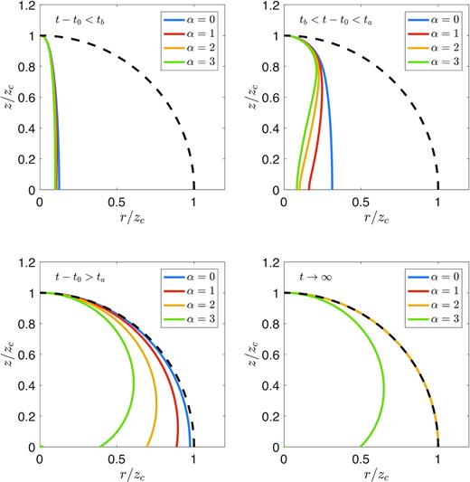
Comparison of the shape of the shock in each phase of the evolution, for a density profile ρ ∝ R−α with α = 0, 1, 2, and 3. The axes are scaled to the height of the cocoon, zc, to allow for an easy comparison. The black dashed line is a sphere of radius zc. Upper left: The planar phase (t − t0 < tb). Upper right: The sideways expansion phase (tb < t − t0 < ta). Lower left: The quasi-spherical phase (ta < t − t0). Lower right: The asymptotic shape as t → ∞; note that the lines for α = 0, 1, and 2 are overlapping because in each of these cases the shock becomes spherical.
The asymptotic behaviour can be divided into two different regimes depending on α. For |$\alpha \leq 2$|, the shock becomes fully spherical and the system is described by the classical spherical ST blast wave solution at late times. Interestingly, however, non-sphericity persists indefinitely in the KA when α > 2. Although the shock still becomes self-similar in this case, it does not become spherical: the shock radius remains smaller at the equator than at the poles, resulting in a peanut-like shape. The reasons for the different shapes will be explored further in Section 3.2.3.
Our model assumes that the pressure in the ambient medium is negligible compared to the cocoon pressure, and that the ambient medium is effectively static, with an expansion velocity much smaller than the shock velocity. If either of these conditions are violated, the solution breaks down. The range of validity of the model is discussed further in Section 3.5.
The fact that ta ∼ (a/b)2t0 implies that an outflow takes much longer to become quasi-spherical if it is initially narrow (i.e. if b ≪ a). This is due to a combination of two effects which cause narrow cocoons to be more strongly decelerated. First, narrow outflows undergo a larger drop in velocity when the jet ram pressure vanishes. After the jet is choked, the on-axis velocity decreases from its initial value, βh, to a new value, ∼βc, which is comparable to the sideways expansion speed. Since a ∼ cβht0 and b ∼ cβct0, the velocity is reduced by a factor of βc/βh ∼ b/a. Secondly, initially narrow cocoons are more strongly affected by sideways expansion. As discussed above, the width of the outflow grows from b to ∼a in the time it takes the height to double. This increases the volume by a factor of ∼(a/b)2, and decreases the pressure by a factor of ∼(b/a)2. Since |$v_z \propto P_{\rm c}^{1/2}$|, the sideways expansion reduces the velocity by an additional factor of (Pc/P0)1/2 ∼ b/a, so by the time the shock reaches a height of 2a, the on-axis velocity is only vz ∼ (b/a)cβc ∼ (b/a)2cβh.
3 ANALYTICAL SOLUTIONS FOR COCOON EVOLUTION
To help keep track of the many definitions employed throughout this paper, we provide a list of the symbols used in Appendix A, along with their meaning and the place in the text where they are defined. In naming variables, we make use of the following subscripts to simplify our notation:
The subscript ‘0’ refers to values measured at the choking time, t = t0.
Global properties of the cocoon (such as its height, volume, and pressure) which depend only on time are marked with the subscript ‘c’.
Quantities pertaining to the ‘bulge’ (a special point on the cocoon surface where the instantaneous velocity is parallel to the equator; see Section 3.2) are denoted by the subscript ‘b’.
Parameters characterizing the jet prior to choking are subscripted with a ‘j’.
Finally, various constants that depend on the density profile are given the subscript ‘α’.
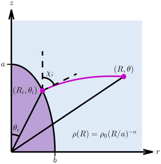
Problem setup. A high-pressure cocoon (purple) expands into an external medium (blue). In a power-law density profile, particles at (Ri, θi) travel along the curved pink path to reach the point (R, θ). The initial direction of motion is perpendicular to the shock surface; the angle between the axis and the surface normal is χi.
Now, suppose that at t = t0 the gas within the cocoon has a pressure P0, distributed uniformly over a volume V0. At each point along the shock surface, the internal pressure applies a force in the direction normal to the surface. The speed v of a surface element is set by balancing the mass and momentum flux in a frame comoving with the shock, leading to v = [(γ + 1)P′/2ρ]1/2, where P′ is the post-shock gas pressure. The ambient pressure is assumed to be negligible compared to the ambient ram pressure.
The speed in the direction normal to the surface can alternatively be derived geometrically. Consider a point on the shock surface with speed |$\boldsymbol {v}$| which travels from an initial angular position (R, θ(R, t)) to a new position (R + dR, θ(R + dR, t + dt)) in time dt. The displacement vector |${\rm d}\boldsymbol {s}$| connecting the initial and final points is normal to the surface and has a magnitude of ds = vdt. If the shock is inclined by an angle ω with respect to the radial direction, the radial component of the displacement is given by dR = dscos ω. We now decompose the displacement vector into two components: the first, |${\rm d}\boldsymbol {s}_1$|, goes from (R, θ) to (R + dR, θ(R + dR, t)) with t held fixed, and the second, |${\rm d}\boldsymbol {s}_2$|, goes from (R + dR, θ(R + dR, t)) to (R + dR, θ(R + dR, t + dt)) with R held fixed. On the first path, R changes by dR = dscos ω, and θ changes by |$(\partial \theta /\partial R) {\rm d}R$| (since t is fixed), so the total path-length is |${\rm d}s_1= {\rm d}s \cos \omega \sqrt{1+ R^2 (\partial \theta /\partial R)^2}$|. On the second path, R is held constant and therefore the path-length is |${\rm d}s_2=R |\partial \theta /\partial t| {\rm d}t= (R/v) |\partial \theta /\partial t| {\rm d}s$|. To complete the derivation, we note that the angle between |${\rm d}\boldsymbol {s}_1$| and |${\rm d}\boldsymbol {s}_2$| is ω, and that |${\rm d}\boldsymbol {s}_1$| is tangent to the surface and perpendicular to |${\rm d}\boldsymbol {s}$|. Therefore, the vectors |${\rm d}\boldsymbol {s}$|, |${\rm d}\boldsymbol {s}_1$|, and |${\rm d}\boldsymbol {s}_2$| form a right triangle such that ds1/ds2 = cos ω. Substituting the values of ds1 and ds2 in this equation results in |$v = R |\partial \theta /\partial t| [1+ R^2 (\partial \theta /\partial R)^2]^{-1/2}$|.
It is possible for x to be bounded or unbounded, depending on whether integral in equation (18) converges or diverges as t → ∞ (see also Section 3.4). Since we expect to recover the ST solution at late times, with R ∝ t2/(5 − α) and Pc ∝ R−3 ∝ t−6/(5 − α), we find that the integral diverges for |$\alpha \leq 2$|. The transition to the sideways expansion phase discussed in Section 2 occurs at x ∼ b/a, while the transition to the quasi-spherical phase occurs when x ∼ 1.
As we will see, the evolution of the cocoon depends strongly on α, the power-law index of the external density profile. We begin by discussing the simple case of a constant ambient density as an illustrative example. Then, we examine how the evolution changes as the external density profile steepens.
3.1 A constant external density
When the external density is uniform with ρ(R) = ρ0, each point along the shock surface travels with the same velocity, v(t) = [(γ + 1)Pc(t)/2ρ0]1/2, since all points are driven by the same uniform pressure into the same density. Furthermore, since there is no differential velocity between adjacent points on the surface, each small patch of surface maintains its original orientation. Therefore, a particle on the surface travels to infinity along a straight line in the direction normal to the surface. Examining equation (19), we see that it reduces to x(t) = ∫v(t)dt/a in the constant density case. In other words, when α = 0, the distance travelled along each trajectory at time t is simply ax(t). Thus, a particle beginning at (Ri, θi) at time t0 travels a distance ax along a straight line to reach a new position (R, θ) at time t, as illustrated in Fig. 3.
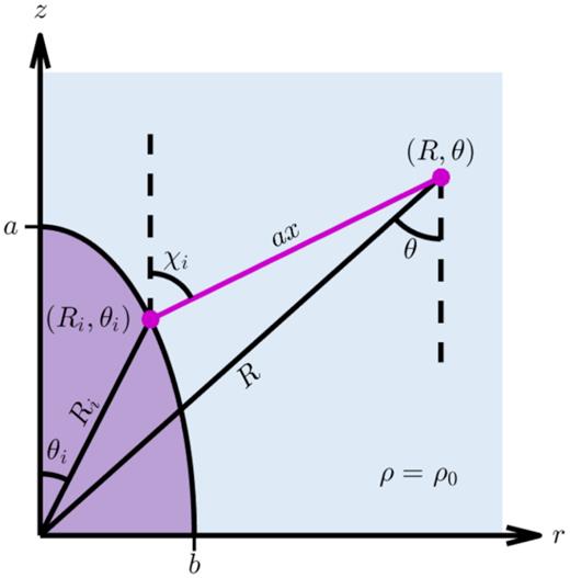
As in Fig. 2, but for a uniform density ρ = ρ0. Particles follow a straight-line trajectory from (Ri, θi) to (R, θ), covering a distance ax. A triangle of side lengths Ri, R, and ax is formed by connecting the starting location, the new location, and the origin. The interior angle opposite to R is given by |$\pi -(\chi _i-\theta _i)$|.
As x → ∞, the outflow becomes gradually wider and rc/zc → 1 while ϵeff → 0. In fact, we see from equation (21) that for large x, R ≈ ax regardless of θi, indicating that the cocoon becomes spherical. Taking x ∝ R and Pc ∝ Vc ∝ R−3 in equation (18), we see that the usual R ∝ t2/5 behaviour for a blast wave in a constant density is recovered.
The solution for α = 0 is plotted in Fig. 4 at the times when the cocoon’s height has reached 2, 4, 6, 8, and 10 times its initial value. The initial shape was taken to be an ellipsoid with aspect ratio b/a = 0.2. Several particle paths are also indicated. A few key properties of the constant-density solution are worth emphasizing. First, all of the trajectories are straight lines that do not cross. There are no self-intersections of the cocoon surface. Secondly, the width of the outflow is always a maximum in the equatorial plane. Finally, the solution gradually approaches a self-similar spherical blast wave as t becomes large. The process of becoming spherical is relatively rapid: by the time the cocoon’s height has doubled to zc = 2a, equation (27) shows that its width is already rc > zc/2, regardless of how narrow it was to start. As we will see, these basic features do not necessarily hold true at higher α.
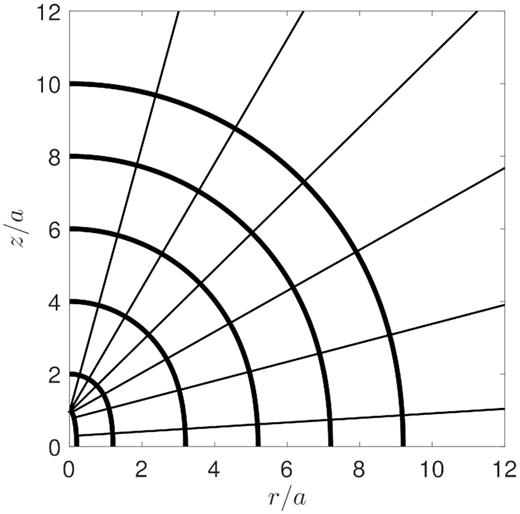
The shape of the cocoon (thick lines) when zc/a = 1, 2, 4, 6, 8, and 10, for a constant density profile with α = 0 and a/b = 5. Several trajectories for different starting points on the cocoon surface are also shown as thin lines.
3.2 A power-law external density
In a non-uniform, spherically symmetric density profile, there is a density gradient in the radial direction that is not aligned with the surface normal. Although each small patch of the surface is driven from behind by a uniform pressure, adjacent points encounter different densities, feel different ram pressures, and therefore move with different speeds. As a result, elements of the surface change their orientation as they travel outwards, following trajectories that curve towards higher density. The strength of this effect depends on the misalignment of the density gradient and the surface normal, which is expressed by |χi − θi|. The cocoon becomes more deformed in regions where |χi − θi| is larger, eventually developing a bulge near the location where |χi − θi| is maximal.
Because the bulge forms at a larger radius where the density is lower, it expands sideways faster than material in the equatorial plane, and eventually overtakes it. Thus, unlike the constant-density case, in decreasing density profiles the cocoon’s width is ultimately set by the behaviour of the bulge, not the expansion near the equator. Once the bulge has formed, we can describe the cocoon’s shape with four quantities: the extent along the z-axis, zc; the width in the equatorial plane, req; and the coordinates Rb and θb indicating the location of the bulge, which we define to be the point where the cocoon surface is locally parallel to the axis. This point is located at a height zb = Rbcos θb above the equatorial plane and at a distance rb = Rbsin θb from the axis. The cocoon width is then rc = max(rb, req). This configuration is illustrated in Fig. 5.
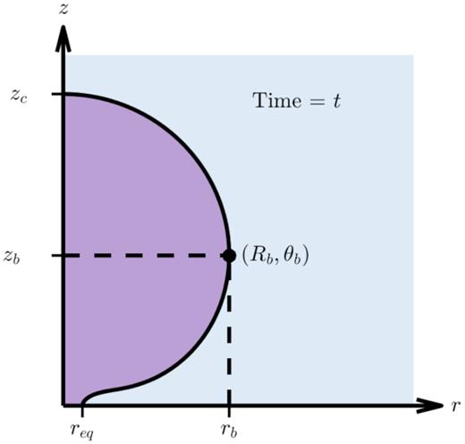
The quantities zc, rb, zb, and req that characterize the cocoon shape. We define the cocoon width rc to be the larger of rb and req (in this case, rc = rb).
The determination of req comes with an important caveat. Because the points on the surface follow curved paths, self-intersections can occur in a non-uniform density profile: when any part of the cocoon reaches the equator, it encounters material coming from the opposite side due to the reflective symmetry of the system. Collisions at the equator are expected to generate a high-pressure region and drive a shock outwards in the equatorial plane. Our simple KA model does not take equatorial interactions into account, and therefore underestimates the true equatorial width. In addition, there is a cusp at the equator in the idealized model which is unlikely to exist in reality. These discrepancies are clearly seen in a comparison with numerical simulations (see Section 5). While the analytically obtained value of req is only accurate to within a factor of a few, it may none the less be useful as a lower bound.
The angle ψi between the axis and the initial direction of motion in ξ–ϕ coordinates can be derived as follows. We first observe that the quantity dln R/dθ = dln ξ/dϕ is preserved by the coordinate transformation. Then, we note that in order for the slope of a trajectory to be |$\cot \chi _i$| at the point (Ri, θi), the initial condition |${\rm d}\ln R/{\rm d}\theta =\cot (\chi _i-\theta _i)$| must be satisfied at θ = θi. By the same logic, |${\rm d}\ln \xi /{\rm d}\phi =\cot (\psi _i-\phi _i)$| when evaluated at ϕ = ϕi. Thus, we have |$\cot (\psi _i-\phi _i)=\cot (\chi _i-\theta _i)=\cot \omega _i$|, and therefore ψi = ϕi + ωi (up to a phase that we choose to be zero).
Equation (35) can be used to derive parametric equations for the coordinates of the bulge. To do so, we first note that since Rb and θb describe a particular point on the cocoon’s surface, they must be functions of time alone, i.e. Rb = Rb(x) and θb = θb(x). The trajectory passing through the point (Rb(x), θb(x)) at a given time x can be traced back to a specific initial angular position θb0(x), as shown in Fig. 6. That is to say, for each time x, there exists a corresponding initial angle θb0(x) such that R(x, θb0(x)) = Rb(x) and θ(x, θb0(x)) = θb(x). The relationship between x and θb0 is derived in Appendix B, but the exact functional form is not important for this discussion. For now, it suffices to say that there is a one-to-one mapping between θb0 and t. Therefore, θb0 can be thought of as an alternative dimensionless time parameter, which has an initial value of |$\theta _{\rm b0}=\pi /2$| and decreases monotonically to a final value θb0, min as t → ∞.
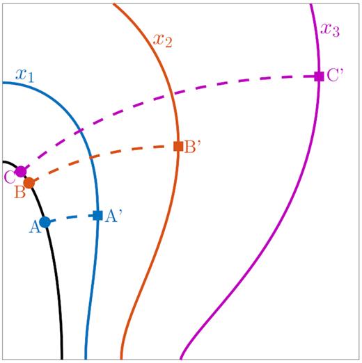
The shape of the shock at three times – x1 (blue), x2 (red), and x3 (magenta) – taking α = 2 and b/a = 0.3 as an illustrative example. The coloured squares mark the location of the bulge where the velocity is parallel to the equator. The angular coordinates of the points A’, B’, and C’ are, respectively, θb(x1), θb(x2), and θb(x3). At each time, the dashed trajectory passing through the bulge can be traced to a unique point on the initial surface, as indicated by the filled coloured circles along the black curve. The points labelled A, B, and C have initial angular positions of θi = θb0(x1), θb0(x2), and θb0(x3) respectively.
We thus conclude that x is not, in general, a suitable choice of parameter for comparing rc and zc in a non-uniform density. What, then, would be a better choice? The discussion surrounding equations (36)–(37) suggests another option: parametrizing the system in terms of θb0. This turns out to be a good choice, in the sense that the important quantities characterizing the cocoon’s shape (zc, rb, and zb; see Fig. 5) can be written explicitly in terms of θb0 and the quantities Rb0 and χb0 derived from the initial shape. For clarity of presentation, we reserve the derivation of the full system of parametric equations describing the shape for Appendix B.
The new parametrization allows a direct comparison between the height zc(θb0) and the width rc(θb0) of the cocoon at a given time x. However, a drawback compared to the constant-density case is that the equations cannot be solved to obtain an explicit function rc(zc) relating the height and width. None the less, it is possible to simplify the exact equations to obtain an approximate relation between rc and zc in each of the dynamical regimes discussed in Section 2 (see Appendix C). Expressions relating req and zc can also be derived in a similar manner (see Appendix D), although there are issues with the KA near the equatorial plane as discussed above.
Here, we give only a qualitative overview of the results, assuming an initially ellipsoidal shape as given by equation (13). In this case, the cocoon width is initially set by the ejecta in the equatorial plane, with rc = req. We find that the evolution of rc depends on the relationship between α and the outflow’s initial aspect ratio, a/b. If |$\alpha \leq 2b^2/a^2$|, no bulge develops, and the outflow remains widest at the equator indefinitely, similar to the constant-density case. In this scenario, there are no trajectories which pass through the equator, so there is no interaction between ejecta from opposite sides of the equator. On the other hand, if α > 2b2/a2, the bulge eventually forms and overtakes the equatorial ejecta, and collisions at the equator occur as well.
We are mainly interested in the scenario where a/b ≫ 1, in which case α ≫ 2b2/a2 also holds unless the density profile is very flat. In this limit, the bulge overtakes the equatorial material early in the planar phase, once the width has increased by rc − b ≈ (2b2/αa2)b ≪ b. The cocoon’s width is therefore governed by the behaviour of the bulge, with rc = rb for the majority of the evolution. The motion of the bulge during each dynamical phase can be summarized as follows:
During the planar phase, the bulge initially remains close to the equator. At first, particles have not had sufficient time to significantly change their direction of motion, so the cocoon width is determined by the ejecta from θb0 ≫ b/a, which had an initial velocity almost perpendicular to the axis, with |$\chi _{\rm b0}\approx \pi /2$|. As the cocoon expands, material at larger z (which started closer to the axis, but with a higher speed due to the lower density) begins to overtake material at smaller z, causing the bulge to march along the surface towards smaller θ. By the time the cocoon’s width has doubled, the bulge has crossed most of the surface, with θb decreasing from |$\sim \pi /2$| to ∼b/a.
In the sideways expansion phase, the particles at the location of the bulge originated from b2/a2 ≪ θb0 ≪ b/a. On this part of the surface, the r- and z-components of the initial velocity are comparable, with |$\chi _{\rm b0}\gtrsim \pi /4$|. The particles in the bulge have had to change their direction of motion by ≲45 deg, moving farther from the axis in the process. By the time a particle starting from θb0 passes through the bulge, its angular position has increased to θb ≫ θb0. Because the width of the outflow increases in this phase, while the height stays about the same (see Section 2), θb now grows over time. This phase ends when the height and width of the cocoon become comparable, at which point θb ∼ 1.
- Finally, during the quasi-spherical phase, the width is governed by material that came from θb0 ≪ b2/a2. The material in the bulge was initially moving almost parallel to the axis, with |$\chi _{\rm b0}\ll \pi /4$|, and had its direction of motion changed by ∼90 deg. As in the previous phase, θb ≫ θb0. As time goes on, the value of θb continues to gradually increase. Eventually, the evolution becomes scale-free, with all length-scales ∝ zc. However, the outflow does not necessarily become spherical in the KA, as we discuss in Section 3.2.3. To capture the shape at infinity, we define two constants of proportionality depending on α, fα, and gα, such thatIn addition, we define the maximum angle reached by the bulge as(39)$$\begin{eqnarray*} \begin{array}{ll}f_\alpha \equiv \lim _{t \rightarrow \infty } (r_{\rm c}/z_{\rm c}) \\ g_\alpha \equiv \lim _{t \rightarrow \infty } (r_{\rm eq}/z_{\rm c}) \end{array} . \end{eqnarray*} $$If the outflow becomes spherical, then fα = gα = 1, and the bulge moves to the equator so |$\theta _{\rm b \infty }= \pi /2$|. Otherwise, we have fα < 1 and gα < 1, with fα ≠ gα, and |$\theta _{\rm b \infty }\lt \pi /2$|.(40)$$\begin{eqnarray*} \theta _{\rm b \infty }\equiv \lim _{t\rightarrow \infty } \theta _{\rm b}. \end{eqnarray*} $$
The approximation used to generate equation (41) is equivalent to assuming that the shock was generated by a point explosion placed at z = a. Although K92 did not explicitly give an equation for R(θ, x) in the point explosion case, equation (41) can be reproduced by combining the two expressions given in their equation (23). As with other results derived from the KA, equation (41) is expected to be less accurate towards the equator.
While the evolution during the planar and sideways expansion phases is not affected much by the density gradient, the asymptotic behaviour of the outflow depends strongly on the density profile. Two different scenarios are possible, depending on whether the density profile is shallow (α < 2) or steep (α > 2). We discuss each regime in turn below, along with the special case α = 2. As before, we treat only the specific case of an initially ellipsoidal shock.
3.2.1 A shallow external density profile (0 < α < 2)
For α < 2, k is positive, and the integral in equation (18) diverges so x → ∞ as t → ∞. Inspecting equation (38), we see that |$z_{\rm c}\propto x^{1/k_\alpha }\propto x^{2/(2-\alpha)}$| for large x. Assuming that the pressure drops as |$P_{\rm c}\propto V_{\rm c}\propto z_{\rm c}^{-3}$| asymptotically, equation (18) implies x ∝ t(2 − α)/(5 − α). Thus, as expected, we recover a blast wave evolution with zc ∝ t2/(5 − α) at late times.
As discussed above, interactions at the equator occur in a non-uniform external density when α > 2b2/a2. Which regions on the cocoon surface eventually experience a collision? For 2b2/a2 < α < 2, it turns out that θb0 has a minimum value θb0, min > 0. Trajectories stemming from θb0, min are asymptotically parallel to the equator, i.e. they have |$\theta \rightarrow \pi /2$| as x → ∞. Particles originating from θi < θb0, min follow paths that never become parallel to the equator, so they can never be located at the bulge’s location. These particles stream freely to infinity, without interacting with any other ejecta. On the other hand, particles with θi > θb0, min eventually undergo a collision at the equator. The value of θb0, min is derived in Appendix C.
The shape of the cocoon at z/a = 2, 4, 6, 8, and 10 is shown in Fig. 7, for α = 1 and b/a = 0.2. The trajectory stemming from θb0, min and the evolution of the bulge’s location are also shown, respectively, as dotted and dashed lines. To summarize, as in the constant density solution, the flow becomes more spherical with time, eventually becoming a self-similar ST blast wave. However, in contrast with the constant-density case, if α > 2b2/a2 a portion of cocoon material with θi > θb0, min eventually reaches the equator and experiences a collision. Furthermore, whereas for a constant density the cocoon is always widest at the equator, for a decreasing density profile, the cocoon bulges out and its width is maximum at some height zb > 0. But, because zb grows more slowly than zc, zb/zc steadily decreases and the relative position of the bulge gradually approaches the equator at late times.
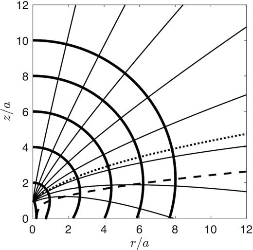
As in Fig. 4, but for α = 1. The dotted line separates trajectories that eventually reach the equator and collide with cocoon material from the other side, from those that proceed freely to infinity without interacting. The dashed line shows the curve Rb(θb), which always passes through the cocoon surface at its widest point.
3.2.2 A wind-like external density profile (α = 2)
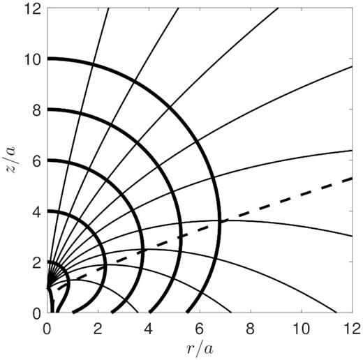
Cocoon shapes and particle trajectories for α = 2 are shown in Fig. 8, using the same values as before for zc and b/a. The dashed line, which tracks the position of the bulge in space, would become horizontal for a spherical flow. The extremely gradual change in the slope of this line captures the slow transition to sphericity.
3.2.3 A steep external density profile (2 < α < 3)
In Fig. 9, we plot the cocoon’s shape and several trajectories for α = 3. Compared to the previous cases, the trajectories are more curved. Also, because of the steep density gradient, the density near the tip is much lower than the density near the base. As a result, material originating near the axis wraps around and actually reaches the equator before material on the sides. The path traced out by the bulge (dashed line) straightens out and never becomes parallel to the equator, as expected for an outflow which does not become spherical.

We emphasize again that the above results are based on an idealized model that ignores heating due to collisions between ejecta from opposite hemispheres at the equator. The effects of equatorial interactions will tend to make the outflow more spherical than what the analytical model predicts. Interactions may be particularly important for steeper density profiles, because whereas in relatively flat density profiles the equatorial collisions are glancing, in steep density profiles they can occur head-on (see Appendix D). This can be seen in Fig. 9: the first ejecta to reach the equator follow the dot–dashed path and collide fully head-on with material from the other side. The other paths in Fig. 9 also intersect the equator at a steep angle ≳45 deg. In comparison, the trajectories in the α = 1 case (Fig. 7) approach the equator at a much shallower angle and interact more weakly.
As a final note, we point out that for sufficiently steep α, there can be a region inside the cocoon, located along the equator, which is never shocked in the analytical model. This is simply a mathematical feature of the idealized KA model, which is not present in numerical simulations (see Section 4), and which most likely does not exist in reality. In a more realistic model taking the interaction between ejecta colliding at the equator into account, we expect that a pressure gradient would develop due to collisions on either side of the unshocked region, which would then drive material into this region and shock it. In any case, because the unshocked region is engulfed by the rest of the cocoon, its presence or absence does not affect our conclusions about the late-time behaviour.
Asymptotic cocoon properties for the regimes discussed in Section 3.
| |$\alpha \leq 2b^2/a^2$| | 2b2/a2 < α < 2 | α = 2 | 2 < α < 3 | |
|---|---|---|---|---|
| |$(k_\alpha \geq 1-b^2/a^2)$| | (0 < kα < 1 − b2/a2) | (kα = 0) | (− 1/2 < kα < 0) | |
| fα | 1 | |$\left[\sin (\pi /\alpha)\right]^{\alpha /(\alpha -2)}$| | ||
| Aα | |$\left(2/k_\alpha ^2\right) \sin ^2(k_\alpha \pi /4)$| | |$\pi ^2/8$| | |$\left(1/2k_\alpha ^2\right) \cot ^2(\pi /\alpha)$| | |
| ζ | |$(1/k_\alpha)\left[(z_{\rm c}/a)^{k_\alpha }-1\right]$| | ln (zc/a) | |$(-1/k_\alpha)\left[(z_{\rm c}/a)^{-k_\alpha }-1\right]$| | |
| Bulge forms? | No | Yes | ||
| Asymptotic shape | Sphere | ‘Peanut’ | ||
Fig. 10 compares the limiting expressions in (67) with the full solution for each of the values of α discussed above. We see that when α is not too close to 2, the asymptotic approximation agrees well with the exact solution for zc ≳ 10a. For α ≈ 2, however, the leading-order approximation given in equation (67) becomes less accurate. The reason for the slow convergence is that, since ζ ∝ ln zc for α = 2, the contribution from higher order terms in ζ is non-negligible. If greater accuracy is required, the parametric equations presented in Appendix B can be used to calculate rc/zc instead.
The ratio rc/zc as a function of cocoon height, for b/a = 0.03 and α = 0, 1, 2, and 3. The dotted and dashed lines show the approximations given in equation (67), respectively, in the limits zc − a ≪ a and zc ≫ 2a.
3.3 The volume of the cocoon
The integral in equation (70) can be evaluated analytically in limited cases, but it is generally more convenient to evaluate it numerically. In Fig. 11, we plot Cα as a function of α, and compare it to the value of |$3V_{\rm c}/\left(4\pi z_{\rm c}^3\right)$| found by direct numerical integration of equations (33) and (34) at zc/a = 10, 100, and 1000. As expected from the results of Section 3.2, the α = 2 case is slowest to converge to the limiting volume, while for α ≲ 1, the asymptotic expression is already a reasonably good approximation for zc ≳ 10a. Additionally, we plot the estimate |$C_\alpha \simeq f_\alpha ^2$| obtained by treating the cocoon as an ellipsoid with volume |$(4/3)\pi r_{\rm c}^2 z_{\rm c}$|. Replacing Cα by |$f_\alpha ^2$| is reasonably accurate, and has the advantage of being easy to compute via equation (62).
The volume of the cocoon scaled to |$4 \pi z_{\rm c}^3/3$|, as a function of α for b/a = 0.1. The blue, red, and yellow curves depict the volume when the cocoon has expanded to 10a, 100a, and 1000a, respectively. The limiting value as zc → ∞ is shown in black: the solid line is the accurate value given by equation (70), while the dotted line is the simple approximation |$C_\alpha \simeq f_\alpha ^2$|.
3.4 The age of the cocoon
In Fig. 12, we plot the analytical estimates in equations (76) and (77), compared to the accurate result obtained from numerical integration of the dynamical equations. We choose a small value of b/a = 0.03 so that the intermediate regime shows up clearly. In general, the formulae in (76) and (77) do a good job at reproducing the full solution.

The time it takes for the cocoon’s width to become 60 (yellow), 80 (red), and 90 (blue) per cent of its height, as a function of α, for an initially ellipsoidal cocoon with a/b = 10. All times are scaled to the time for the height to double, |$t_a \simeq \sqrt{2} (a/b)^2 t_0$|. The solid blue line shows the numerically calculated value of Qα, while the dashed line represents the analytical estimate given by equation (79).
3.5 Eventual breakdown of the solution
In this section, we estimate the time at which the KA solution breaks down. The KA model makes two key assumptions which may eventually become invalid. First, the shock is assumed to be strong. In a static medium, this condition holds until the outflow reaches pressure equilibrium with the surrounding medium, on a time-scale teq. In an expanding medium, on the other hand, the shock becomes weak once the shock velocity becomes comparable to the expansion velocity of the ambient gas, which takes a time tw. Secondly, the model assumes that the ambient medium extends to infinity. If the extent is finite, then the solution is valid only up until the time tbo when the shock breaks out. The KA model applies up until t = min (teq, tw, tbo).
The eventual fate of the outflow depends on the ordering of the time-scales discussed above. We investigate three astrophysically relevant scenarios: a GRB jet choked inside a WR star (i.e. a failed long GRB); a GRB jet choked within an extended, low-mass stellar envelope (as may be the case in llGRBs); and an AGN jet in a cluster environment choked by the intracluster medium. In each case, the ambient medium can be treated as static. Therefore, the relevant time-scales are ta, teq, and tbo.
In a typical long GRB, it takes the jet ∼15 s to drill through the progenitor WR star (Bromberg et al. 2012). Therefore, we expect jets with a duration of ∼ a few seconds to be choked at an appreciable fraction of R*, i.e. we have a/R* ∼ a few tenths. In this case ηbo is order-unity and tbo ∼ ta. A WR star can be approximated by an n = 3 polytrope, with the ambient density and pressure scaling as ρ ∝ R−5/2 and Pa ∝ ρ4/3 ∝ R−10/3 in the outer parts of the star. As PaR3 ∝ R−1/3 changes slowly with radius, the quantity Pa0a3 appearing in equation (82) is roughly constant, regardless of the choking location. Numerical modelling of pre-supernova stars (e.g. Heger, Woosley & Spruit 2005) suggests a pressure of the order of |$2 \times 10^{18}\, \text{erg cm}^{-3}$| at R = 1010 cm. We then have |${\eta _{\rm eq}\simeq 80 (E_0/10^{51}\, \text{erg})(P_{\rm {a0}}a^3/10^{48}\, \text{erg})^{-1} \gg 1}$|. Thus, ta ∼ tbo ≪ teq, and the breakout occurs while the KA model is still valid.
The progenitors of llGRBs, on the other hand, may have an extended optically thick envelope containing a mass |$\sim 10^{-2} \, \mathrm{M}_{\odot }$| within a radius ∼100–1000 R|$\odot$| (Campana et al. 2006; Nakar 2015; Irwin & Chevalier 2016). The pressure in this envelope is unknown, but it must be smaller than in the WR star case, since the envelope is both cooler and less dense. We then expect ηeq ≳ 100, as before. However, because of the larger radius compared to the WR star case, a typical GRB jet is choked deep within the extended envelope, with a/R* ≪ 1. We therefore have ηbo ≫ 1 and a quasi-spherical breakout occurs at tbo ≫ ta. Assuming that the jet successfully escapes the star, a is at least ∼10 R|$\odot$|, so ηbo is at most ∼100. We then find ta ≪ tbo < teq, so in this case the KA model also applies up until breakout.
In AGNs, buoyancy will also become important at late times. The effects of buoyancy are discussed in more detail in a separate paper (Irwin et al. 2019), where we apply the model to young bubbles inflated by jets in galaxy clusters. Here, we simply remark that if the ambient medium is in hydrostatic balance, and the size of the bubbles is comparable to their distance from the central source, the buoyancy time-scale tbuoy is comparable to teq (Churazov et al. 2001; Irwin et al. 2019).
4 INFERRING THE JET PARAMETERS FROM THE COCOON PROPERTIES
For a cocoon formed by a choked jet expanding with a non-relativistic velocity, the initial conditions of the cocoon (a, b, and E0) are related to the parameters of the original jet (the luminosity Lj, the duration tj, and the initial opening angle θop) in a straightforward way. In this section, we consider how to work backwards from the observed characteristics of the cocoon to obtain useful constraints on the initial jet properties. We will assume that it is possible to estimate the cocoon’s height (zc), width (rc), and energy (E0) from observations, and additionally that the density profile is known. The calculation then proceeds in two steps. First, we use the KA model to estimate the age of the system and determine the height and width upon choking (a and b). Then, we apply the jet propagation model of Bromberg et al. (2011) to find the jet properties needed to match this initial shape. Throughout this discussion, we ignore order-unity prefactors for simplicity.
We caution that our analysis applies specifically to outflows which are initially narrow with b ≪ a, as expected when the cocoon is inflated by a relativistic jet. When the observed aspect ratio is zc/rc ≫ 1, the association with a jet is not controversial. However, when zc/rc is of order unity, the alternative possibility that the outflow was powered by a wide-angle wind cannot be ruled out.
The initial width, however, is more difficult to determine. In the quasi-spherical regime, the shape has little to no dependence on the initial width, so b cannot be recovered. In the sideways expansion phase, there is a weak dependence on b, but there is also another issue, which is that the sideways expansion and planar cases are difficult to distinguish observationally. One indication that the cocoon is in the sideways expansion phase is a bulging out towards the tip, as seen in Fig. 1. However, without knowing the initial shape, this method is unreliable, and moreover it only applies when the density profile is fairly steep. With good observations, a better way to test which case is relevant is to compare the strength of the shock along the axis to the strength near the widest part of the cocoon. If the shock is significantly stronger towards the axis, it would be good evidence for a recently quenched jet, suggesting a planar evolution with t ∼ t0 and b ∼ rc.
Now that we have established how a and b depend on the observables, let us consider how they relate to the properties of the original jet. Suppose the jet is injected relativistically with luminosity Lj and opening angle θop, and operates for a duration tj. Bromberg et al. (2011) showed that the dynamics of the jet are governed by a dimensionless quantity |$\tilde{L}$|. At the time t = t0 when the jet is choked, |$\tilde{L} = \text{max}\left\lbrace \left(\frac{L_{\rm j}}{\rho _0 t_0^2 \theta _{\rm op}^4 c^5}\right)^{2/5}, \frac{L_{\rm j}}{\rho _0 t_0^2 \theta _{\rm op}^2 c^5} \right\rbrace$|. The jet is collimated with a non-relativistic head when |$\tilde{L} \ll 1$|; collimated with a relativistic head when |$1 \ll \tilde{L} \ll \theta _{\rm op}^{-4/3}$|; and uncollimated with a relativistic head when |$\tilde{L} \gg \theta _{\rm op}^{-4/3}$|. |$\tilde{L}$| is closely related to the head velocity βh, with |$\beta _{\rm h}\approx \tilde{L}^{1/2}$| for a non-relativistic jet, and |$2 \Gamma _\mathrm{ h}^2=\tilde{L}^{1/2}$| for a relativistic head, where |$\Gamma _\mathrm{ h} \approx (1-\beta _{\rm h}^2)^{-1/2}$|.
The case of an uncollimated jet can be further subdivided depending on the relative values of |$\tilde{L}$| and |$\theta _{\rm op}^{-4}$|. If |$\tilde{L} \ll 4 \theta _{\rm op}^{-4}$|, the jet and cocoon are in causal contact and the pressure in the cocoon remains more or less uniform. However, if |$\tilde{L} \gg 4 \theta _{\rm op}^{-4}$|, causal connection is lost and the approximation of uniform pressure breaks down. We therefore restrict our discussion to the |$\tilde{L} \ll 4 \theta _{\rm op}^{-4}$| case in which the KA remains valid.
5 COMPARISON WITH NUMERICAL SIMULATIONS
To check the validity of the analytical results, we compared them to numerical simulations carried out by a collaborator, O. Gottlieb, using the publicly available hydrodynamics code pluto (Mignone et al. 2007). The axisymmetric simulation setup is akin to previous studies of GRB jet propagation (e.g. Gottlieb et al. 2018; Harrison et al. 2018). The jet is injected with a two-sided luminosity of 1051 erg s−1, a Lorentz factor of 5, and a specific enthalpy of 100 into a nozzle of width 8 × 107 cm for a duration of tj = 3 s. An adiabatic index of 4/3 is used in all cases. The lower boundary of the simulation is placed at zinj = 109 cm, and the external density is defined by ρ(R) = 6 × 10⁴(R/zinj)−α g cm−3. The ambient pressure is set to a negligibly low value.
We compared our results with three simulations, for three values of α relevant to astrophysical jets: α = 1, as is typical for the dense core of a galaxy cluster; α = 2, as expected for a dense circumstellar wind; and α = 2.5, as appropriate in the outer parts of a WR star. Tracer particles are included in the unshocked jet to determine when all of the jet material has flowed into the cocoon. Once all the jet has been shocked, the maximum speed of the tracers drops. In each simulation, we locate the time-step where this drop occurs and call this the choking time. We then find the height, width, and volume-averaged pressure of the outflow at the choking time, and use these as initial conditions for the analytical model. From there we evolve the analytical cocoon model according to Section 3, assuming a nominal value of λ = 1 in equation (16).
The simulation results are shown in Figs 14, 15, and 16 respectively, for α = 1, 2, and 2.5. The analytical solution obtained from the KA at each time is also shown in a heavy black line. In the α = 1 and α = 2 cases, there is good agreement (within 10–15 per cent) between the analytical and numerical results out to about 45 deg from the axis. The slight disagreement is due to the fact that the pressure behind the shock in the simulations is slightly larger than assumed by the KA. The shapes can be made to agree by adjusting the parameter λ, with λ ≈ 1.2 giving an improved fit.
pluto simulations of a choked relativistic jet in a ρ ∝ R−1 density profile. Snapshots are shown at t = 36, 116, and 220 s, when the outflow has reached heights of roughly 2, 3, and 4 × 1010 cm. The colour scale indicates log pressure in units of dyne cm−2. The analytical solution obtained from the KA is shown for comparison as a heavy black line.
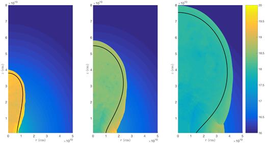
As in Fig. 14, except for ρ ∝ R−2 at t = 13, 37, and 81 s.
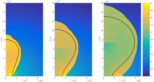
Beyond 45 deg, the shapes start to deviate, and as expected the agreement becomes worse near the equator. Typically, the analytical model underestimates the equatorial radius by a factor of 2–3. As discussed above, one possible source of the discrepancy at the equator is the increased pressure due to collisions. However, another reason that the equatorial radius is larger in the simulations is that the analytical model assumes, following the KA, that the initial pressure is uniform. In the simulations, this is not the case; rather, there is a clear gradient in pressure and velocity at the time of choking, with both being larger towards the equator. One possible reason why the shock might be stronger at large angles is that the ejecta near the equator were shocked at earlier times when the sideways expansion was faster and the density was higher. An alternative possibility is that some interaction at the equator already took place while the jet was active.
In the α = 2.5 case, there are also discrepancies near the equator, for the same reasons discussed above. In addition, the extent along the axis is somewhat larger in the numerical simulation compared to before. This comes about because the analytical model assumes that the outflow has already decelerated to a steady state where the velocity is given by ∼(P/ρ)1/2, or in other words, that the ram pressure of the jet suddenly becomes unimportant at the choking time. It seems that this assumption is reasonable when α = 1 or 2, but not for α = 2.5. This makes sense considering that, prior to choking, the jet head is accelerating in the α = 2.5 case, whereas in the other cases it is decelerating (α = 1) or has a constant velocity (α = 2). Therefore, for α = 2.5, it takes longer for the on-axis ejecta to decelerate and approach the KA prediction. In fact, a shock is clearly visible in Fig. 16, indicating that deceleration is ongoing. Despite the differences on the axis and at the equator, the analytical solution still does a good job at predicting the cocoon’s width to within roughly 10 per cent.
In addition to the jet simulations described above, we also tested our conclusion that the outflow does not become spherical for α > 2. To do so, we compare with the results of a different simulation, in which an ellipsoid filled with a uniform high pressure is placed into a ρ ∝ R−2.5 density profile and allowed to evolve. Since there is no need to resolve a jet in this case, the flow can be tracked to much larger radii, until it becomes approximately self-similar. The initial aspect ratio of the outflow is a/b = 70/3 ≫ 1, and the ambient pressure is set to a small value (10−8 times the initial cocoon pressure) so that it does not affect the evolution.
In Fig. 17, we compare the shape of the cocoon seen in the simulation to the prediction of the analytical model. The figure shows a snapshot of the simulation at t/t0 = 840, when the height is zc/a = 10.4. As expected, we find that the outflow does not become spherical when t grows large. The shape in the analytic model, using the same values of zc/a and b/a, is drawn as a solid black line. The shape observed in the simulations is slightly narrower towards the axis and wider towards the base, but otherwise agrees well with the analytical prediction. In particular, the ratio of the cocoon’s width to its height is extremely close to the analytically predicted value of 0.62.

The shape of the cocoon for a ρ ∝ R−2.5 density profile and an initial aspect ratio a/b = 70/3, at a time t/t0 = 840 when the height is zc/a = 10.4. The colour scale indicates the ratio of the pressure to the initial cocoon pressure. The black lines show the shape of the shock in the analytical model, scaled in two different ways. The solid line is scaled to the same zc/a as the simulation, while the dashed line is scaled to the same t/t0.
However, although the agreement at a given height is very good, the agreement at a given time is noticeably worse. Although the cocoon’s size grows as ∝ t2/(5 − α) in the simulations (as expected), the simulation reaches the quasi-spherical phase more quickly than anticipated analytically. As a result, the size of the cocoon in the simulation is larger than the analytically estimated size at a given time. At late times, the ratio of the sizes approaches a constant value of ≈2.5. For example, whereas the simulations reach a height of zc/a = 10.4 at a time t/t0 = 840, the analytical model predicts a height of only zc/a = 4.2 at this time, as shown by the dashed line in Fig. 17. One possible reason for the discrepancy is the fact that, as discussed above, there is a clear pressure gradient along the cocoon surface in the simulations, with the pressure increasing by a factor of a few towards the equator. The higher pressure towards the sides enhances the lateral expansion at early times, causing the outflow to transition to the quasi-spherical regime sooner than it would if the pressure were constant across the surface.
From these considerations, we conclude that our results describing the shock’s shape as a function of height (i.e. equation 67 and Fig. 10) are rather accurate, while our expressions relating the height and width to time (i.e. equations 76–77, and Fig. 12) are only reliable to within a factor of a few. An accurate calibration of the analytical model to more extensive numerical simulations is reserved as an interesting topic for future study.
6 DISCUSSION AND CONCLUSIONS
Jets which fail to penetrate the surrounding medium are expected to leave behind a narrow cocoon filled with hot gas of almost uniform pressure. To describe the evolution of these systems, we consider an axisymmetric generalization of the ST solution in a power-law ambient density profile ρ ∝ R−α, in which the explosion energy is deposited throughout an elongated region along the polar axis. Applying the Kompaneets approximation (KA), we derive a differential equation governing the shock motion, and solve it to yield analytical expressions for the shape of the shock. For a given curve Ri(θi) describing the initial shock shape, we obtain exact parametric solutions for the shock coordinates R(θi, zc) and θ(θi, zc) as functions of zc, the shock height along the axis. The solutions vary in form depending on α. In addition, we provide simplified expressions for the height, width, and volume of the shock versus time in the case of an initially ellipsoidal cocoon with an aspect ratio a/b ≫ 1, as expected for a jet. Our solution extends the previous work of B11, which describes the dynamics of the system while the jet is active, to times after energy injection has ended.
We find that the evolution of the outflow is characterized by three dynamical regimes, which we call the planar regime, the sideways expansion regime, and the quasi-spherical regime. Two important dynamical time-scales are the time for the outflow’s width to double (tb) and the time for its height to double (ta). For a jet choked at time t0, the planar regime persists until the age is ∼2t0. During this time, dynamical quantities remain roughly constant, and the outflow more or less keeps its original shape. Once t ∼ 2tb ∼ 2t0, sideways expansion starts to become important; the pressure in the cocoon drops and the shock starts to decelerate. The shape also changes, with the cocoon bulging out towards the tip. This is especially pronounced in steep density gradients where there is a large density contrast between the base and the tip. Most of the sideways expansion occurs over the time for the cocoon’s height to double, which is t ∼ ta ∼ (a/b)2t0, where a/b is the aspect ratio of the outflow upon choking. After this, the evolution becomes quasi-spherical, the dependence on the initial shape becomes weak, and the shock’s shape is governed primarily by the density profile. As a/b approaches unity, the two characteristic time-scales (tb and ta) become the same and the usual spherical blast wave solution is recovered.
Although the height (zc) and width (rc) of the cocoon become comparable around ta, the time for them to become equal (to within, say, 10 per cent) can be considerably longer. In general we find that the asymptotic behaviour depends strongly on the density profile. For |$\alpha \leq 2$|, the flow becomes spherical. The convergence to a sphere is slower for steeper density profiles, with the quantity 1 − rc/zc going to zero as |$\propto z_{\rm c}^{(\alpha -2)/2}$| for α < 2, or as ∝ (ln zc)−1 for α = 2. An approximation for the time it takes for the outflow to become spherical in different density profiles is given in equation (79). We find that in a constant-density medium, the flow spherizes after about ∼10ta, while in a wind-like medium it takes ∼1000ta.
In steep density profiles with α > 2, the flow does not become spherical (at least in the idealized case where the KA applies). Instead, the ratio rc/zc converges to a constant value of |${}[\sin (\pi /\alpha)]^{\alpha /(\alpha -2)}$| as |${\propto z_{\rm c}^{(2-\alpha)/4}}$|. As before, the convergence becomes slower as α → 2. For 2 < α < 3, the shape of the shock at infinity is narrower towards the equator, like a peanut.
Comparing the analytical solution with numerical hydrodynamics simulations, we find a generally good agreement for zc/a ≲ a few, even without calibration. We compared our results with realistic simulations of a choked jet for three different density profiles of astrophysical interest, with α = 1, 2, and 2.5. In each case, the height and the width of the outflow estimated analytically match the numerically determined value to within about 15 per cent. The agreement is not so good near the equator, but the KA is known to have issues in that region. In addition, we explored the late-time behaviour in the α = 2.5 case through comparison with a simplified simulation in which an elliptical region is filled with an initially high pressure and left to evolve for 840t0. For zc/a ≫ 1, we find that the size of the simulated outflow is larger than predicted analytically by a factor of ≈2.5. However, when rescaled to be the same size, the analytical and numerical shapes are in close agreement.
The fact that the time-scale to become quasi-spherical is long compared to the working time of the jet is good news when it comes to observational applications, since it means that it is not necessary to catch the system shortly after jet activity ceases in order to meaningfully constrain the jet. The relationship between the parameters of the choked jet model (initial height a, initial width b, and the energy E0) and the parameters characterizing the jet (luminosity Lj, duration tj, and opening angle θop) is discussed in Section 4. By measuring the size and shape of a choked jet outflow, along with its energy, it is in principle possible to work backwards to obtain the initial conditions at the moment of choking, and therefore derive the original jet’s properties. However, because the system quickly becomes insensitive to the initial width, constraining b is difficult in practice, unless we happen to catch the system early on. The situation where only E0 and a can be estimated from observations is expected to be more typical. In this case, the jet parameters are subject to degeneracy and cannot be determined uniquely. None the less, knowing the location where the jet was choked is a powerful constraint, and one which is not attainable in spherically symmetric models.
We conclude by discussing several possible future applications of our results. The first involves quenched AGN jets in galaxy clusters. These jets inflate bubbles filled with shocked jet debris that initially expand supersonically, driving a shock into the ambient medium, and later drift away due to buoyancy. Our model can be used to describe the shape of the forward shock surrounding the bubbles during the early evolution when the shocked jet material has not yet reached pressure equilibrium with the intracluster medium or been deformed by buoyancy. The size, shape, and speed of the forward shock can be directly measured from X-ray observations, and then compared with the predictions of the model to derive constraints on the jet properties. This idea is developed further and applied to 5 AGNs with suitably young bubbles in a separate paper (Irwin et al. 2019).
Another possible application deals with observations of SNe that may have harboured a jet. We envision a scenario where the jet is choked before breaking out of its progenitor star, at a radius a < R* where R* is the star’s radius. The cocoon continues to propagate, eventually breaking out of the star when its height is zc = R*. If the choking does not occur too deep inside the star, the width of the outflow upon breakout, rc, will be small compared to R*, and the mass swept up by the cocoon will also be small compared to the star’s mass M*. Once outside the star, the cocoon is expected to quickly expand sideways and engulf the star due to the much lower density. However, since a typical GRB jet imparts an energy of 1051 erg which is comparable to the SN energy, the cocoon will expand faster than the SN due to its lower mass. Therefore, a prediction for the choked jet scenario is the presence of a small amount of mass (0.01–0.1M*) surrounding the supernova that is moving with a speed several times greater than the bulk SN velocity.
This fast-moving ejecta, which is only visible at early times, may have already been observed in some objects (e.g. Izzo et al. 2019; Piran et al. 2019). Early-time spectroscopy makes it possible to estimate the total mass (Mej) and energy (Eej) contained in this high-velocity component, and can even constrain the distribution of mass with velocity. Eej corresponds to the cocoon energy E0 in our model, while Mej serves as a proxy for the width at breakout, with Mej ∼ M*(rc/R*)2. By applying our results, this information can be translated into an estimate of the choking radius, which provides significant insight into the jet properties. Whether the choked jet model can reproduce the observed mass–velocity distribution in Piran et al. (2019) is an interesting question for future study.
The asphericity of the cocoon also has important implications for shock breakout, where even a small departure from spherical flow can lead to oblique effects that dramatically alter the observed signature (e.g. Matzner, Levin & Ro 2013). Therefore, we typically expect the breakout of a choked jet to look markedly different than a fully spherical shock breakout. At the least, an aspherical breakout will last longer and be fainter than a spherical breakout of the same energy, because it takes some time for the breakout to wrap around from the pole to the equator. The expected changes in the breakout emission when it is powered by a choked jet, rather than a spherical SN explosion, will be addressed in future work.
As these examples show, a 2D analytical model for the shape of the shock in choked jet outflows has a wide variety of astrophysical applications, and offers significant advantages over the standard simplifying assumption of spherical symmetry. The Kompaneets approximation model developed here is a useful tool which is straightforward and inexpensive to implement, without sacrificing too much accuracy. Bridging the gap between the jet phase and the spherical phase of evolution is an important step towards a complete picture of jet dynamics, which will remain important as observations continue to reveal evidence for suffocated jets in diverse astrophysical systems.
ACKNOWLEDGEMENTS
We thank O. Gottlieb, who conducted the numerical simulations discussed in Section 5 and graciously shared his data with us, for his generous assistance; his contributions greatly strengthened the final paper. This research is supported by the Council for Higher Education-Israel Science Foundation (CHE-ISF) I-Core Center for Excellence in Astrophysics. TP is supported by an advanced European Research Council (ERC) grant TReX. This work was supported in part by the Zuckerman STEM Leadership Program. CI and EN were partially supported by consolidator ERC grant JetNS and by an Israel Science Foundation (ISF) grant 1114/17.
Footnotes
Hereafter, to reduce clutter, we refer to Ri(θi) and χi(θi) as simply Ri and θi. These and all other quantities subscripted with ‘i’ should be understood as having an implicit dependence on θi.
Equation (15) is undefined for a spherical flow since in that case |$\partial \theta /\partial t \rightarrow \infty$| and |$\partial \theta /\partial R \rightarrow \infty$|. The equation is more well-behaved in the spherical limit when θ is chosen as the independent variable, i.e. when the shock is described by a curve R = R(θ, t). However, in the general case of an aspherical shock in a spherically symmetric density, it is more convenient to use R as the independent variable, because the density is a function of R, not θ.
From here on, we write θb0(x) as simply θb0.
Interestingly, the asymptotic shape often takes a familiar mathematical form when kα is a rational fraction. For example, when kα = −1/2, the asymptotic shape is a cardioid.
We note that pressure equilibrium can only be achieved if the cocoon pressure falls off more steeply than the ambient pressure; this is true only for α < 3/γa.
The case of |$\alpha \leq \frac{2b^2}{a^2}$| describes the scenario where the cocoon always remains widest in the equatorial plane, as discussed above. The case of |$\alpha \geq \frac{2 a^2}{b^2}$| we do not discuss further, because if a ≫ b, it requires an extreme value of α.
If |$\theta _{\rm b}\gt \pi /2$| for some θb0, the physical interpretation is that trajectories stemming from θb0 never become parallel to the equator.
REFERENCES
APPENDIX A: GLOSSARY OF SYMBOLS
Many of the quantities appearing in our problem evolve in time. Additionally, at a given time, certain quantities such as the shock velocity vary along the cocoon surface. Since each point on this surface had a unique initial angular position, θi, at the moment the jet was choked (see Section 3), we use θi to parametrize the relative position on the shock front. In Table A1, we list the symbols defined throughout the paper, explicitly including any dependence on t or θi in parentheses following each symbol.
Glossary of symbols.
| Symbol | Meaning | Introduced |
| Coordinates | ||
| R, θ | Polar coordinates | |
| r, z | Cylindrical coordinates | |
| Initial conditions | ||
| E0 | Energy of the cocoon | Section 2 |
| a | Initial height of the cocoon | Section 2 |
| b | Initial width of the cocoon | Section 2 |
| P0 | Initial pressure in the cocoon | Section 2 |
| V0 | Initial volume of the cocoon | Section 2 |
| ρ0 | Ambient density at R = a | Equation (11) |
| α | Power-law index of the density profile | Equation (11) |
| kα | Frequently appearing quantity defined by kα ≡ 1 − α/2 | Equation (29) |
| Ri(θi) | Curve describing the shock’s initial shape | Equation (13) |
| χi(θi) | Angle between the axis and the shock’s initial direction of motion | Equations (12) and (14) |
| ωi(θi) | Angle between the shock’s initial direction of motion and the radial direction | Equation (22) |
| Time-scales | ||
| t0 | Time when the jet is choked | Section 2 |
| tb | Time it takes for the cocoon’s width to double | Equation (1) |
| ta | Time it takes for the cocoon’s height to double | Equation (2) |
| tsph | Time for the cocoon’s width to become 90 per cent of its height | Equations (78) and (79) |
| teq | Time to reach pressure equilibrium with the ambient medium | Equations (81) and (82) |
| tw | Time when the solution breaks down in an expanding medium | Equations (83) and (84) |
| tbo(R*) | Time when the cocoon breaks out of an ambient medium extending to R* | Equations (85) and (86) |
| Cocoon properties | ||
| Vc(t) | Volume of the cocoon | Section 2 |
| Pc(t) | Average pressure in the cocoon | Section 2 |
| λ | Dimensionless ratio of post-shock pressure to volume-averaged pressure | Equation (16) |
| x(t) | Dimensionless time parameter used to solve for the shock’s shape | Equation (18) |
| zc(t) | Height of the cocoon | Equation (25) |
| rc(t) | Width of the cocoon | Equation (26) |
| req(t) | Width of the cocoon at the equator | See Fig. 5 |
| ϵeff(t) | Effective eccentricity, i.e. |$\epsilon _{\rm eff}\equiv \sqrt{1-r_{\rm c}^2/z_{\rm c}^2}$| | Sections 3.1 and 3.2 |
| R(θi, t), θ(θi, t) | Parametric equations for the shape of the shock at time t | Sections 3.1 and 3.2 |
| Quantities related to the bulge | ||
| Rb(t), θb(t) | Polar coordinates of the bulge | Equation (36) and (37) |
| rb(t), zb(t) | Cylindrical coordinates of the bulge | See Fig. 5 |
| θb0(t), Rb0(t), χb0(t) | Initial values of θi, Ri, and χi for a trajectory passing through (Rb, θb) | See Fig. 6 |
| Asymptotic quantities | ||
| ζ(t) | Quantity important in the expansion of rc(zc) at infinity | Equation (43) |
| Aα | Coefficient appearing in the expansion of rc(zc) at infinity | Equations (44) and (63) |
| fα, gα | Ratios of rc/zc and req/zc, respectively, as t → ∞ | Equation (39) |
| Cα | Ratio of Vc to |$4\pi z_{\rm c}^3/3$| as t → ∞ | Equations (70) and (71) |
| θb∞ | Value of θb(t) as t → ∞ | Equation (40) |
| θb0, min | Value of θb0(t) as t → ∞ | Section 3.2 |
| Jet properties | ||
| Lj | Jet luminosity | Section 4 |
| tj | Jet duration | Section 4 |
| θop | Jet opening angle at injection | Section 4 |
| βh, Γh | Velocity and Lorentz factor of the jet head upon choking | Section 4 |
| βc | Sideways velocity of the cocoon upon choking | Section 4 |
| |$\tilde{L}$| | Dimensionless parameter governing jet propagation | Section 4 |
APPENDIX B: PARAMETRIC EQUATIONS FOR THE COCOON SHAPE
APPENDIX C: EVOLUTION OF THE COCOON WIDTH VERSUS HEIGHT
Approximate formulae for rc versus zc can be obtained in certain limiting situations where equations (B7) and (B8) simplify. To understand the interesting limiting cases, let us investigate how the three angular scales appearing in equation (B10) (θb, ωb0, and Δb) vary with θb0. (We restrict the discussion here to an initially ellipsoidal cocoon, but the conclusions can be generalized to other initial shapes.) To guide the discussion, we plot χb0, ωb0 ≡ χb0 − θb0, θb, and Δb ≡ θb − θb0 versus θb0 in Fig. C1 for α = 1 (left-hand panel) or 3 (right-hand panel) and a/b = 10. Focusing now on the θb and ωb0 curves, the key features are as follows:
Differentiation of equation (36) implies that θb has a minimum if dχb0/dθb0 = α/2 is satisfied. Applying equation (14), we see that this condition is only fulfilled when |$\frac{2b^2}{a^2} \lt \alpha \lt \frac{2a^2}{b^2}$|. If we assume that b ≪ a, and that |$\frac{2b^2}{a^2} \ll \alpha \ll \frac{2a^2}{b^2}$| holds as well,6 then θb has a minimum value of |$\approx \frac{2b}{a} \sqrt{\frac{2}{\alpha }}$| at |$\theta _{\rm b0}\approx \frac{b}{a} \sqrt{\frac{2}{\alpha }}$|. Away from the minimum, θb rises to |$\pi /2$| at |$\theta _{\rm b0}=\pi /2$|, and to |$\pi /\alpha$| at θb0 = 0.7 If α < 2, θb becomes equal to |$\pi /2$| at θb0 = θb0, min (see below).
ωb0 is determined from equation (14), and its behaviour is straightforward since there is no dependence on α: ωb0 is 0 when θb0 = 0, rises to a maximum value of |$\omega _{\rm b0}\approx \pi /2-b/a$| at θb0 ≈ b/a, and then goes to zero again as |$\theta _{\rm b0}\rightarrow \pi /2$|.
The θb and ωb0 curves have two crossings, one at θb0 ∼ b2/a2, and another at |$\theta _{\rm b0}\sim \pi /4$|. Over the range |$b^2/a^2 \lesssim \theta _{\rm b0}\lesssim \pi /4$|, θb < ωb0; otherwise θb > ωb0.
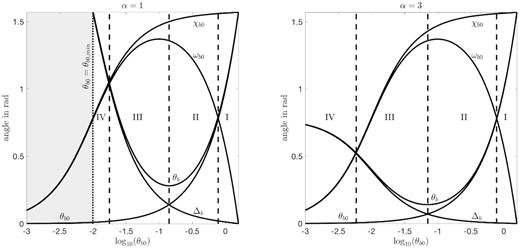
The angular scales θb0, χb0, θb, ωb0, and Δb as functions of θb0, for an initial ellipsoid with b/a = 0.1 and α = 1 (left-hand panel) or α = 3 (right-hand panel). The four dynamical phases described in the text are labelled with Roman numerals and separated by vertical dashed lines. The critical value θb0, min (which is only defined for α < 2) is indicated by a dotted line. The greyed-out region has |$\theta _{\rm b}\gt \pi /2$| and does not affect the evolution of rc/zc.
The outflow’s shape evolves in a different way depending on the relative size of the angular parameters. There are four distinct evolutionary phases (labelled by Roman numerals in the figure) as θb0 is decreased from |$\pi /2$| to θb0, min (when α < 2) or to 0 (when |$\alpha \geq 2$|). These four phases are closely related to the dynamical phases discussed in Section 2. The relationship between the angular scales in each phase is as follows:
Phase I: |$\theta _{\rm b0}\approx \pi /2$| and χb0 > θb0 ≈ θb ≫ ωb0 ≫ Δb. This corresponds to the early planar phase, when x ∼ xb (see also Appendix B), and the bulge is still located close to the equator.
Phase II: |$b/a \ll \theta _{\rm b0}\ll \pi /4$| and χb0 > ωb0 ≫ θb0 ≈ θb ≫ Δb. This applies during the later part of the planar phase, once x ≫ xb and the bulge is closer to the axis than to the equator.
Phase III: b2/a2 ≪ θb0 ≪ b/a and χb0 ≃ ωb0 ≫ θb ≃ Δb ≫ θb0. This holds during the sideways expansion phase.
Phase IV: θb0 → θb0, min or θb0 → 0 (respectively for α < 2 and |$\alpha \geq 2$|), and θb ≈ Δb > χb0 ≈ ωb0 ≫ θb0. This is appropriate in the quasi-spherical phase.
We consider each phase in turn below.
Phase I (|$\theta _{\rm b0}\approx \pi /2$|): Let |$\delta \equiv \pi /2-\theta _{\rm b0}$| be a small quantity. Then, expanding equations (14) and (36) in terms of δ, we find |$\chi _{\rm b0}\approx \pi /2-(b^2/a^2)\delta$|, ωb0 ≈ (1 − b2/a2)δ, |$\theta _{\rm b}\approx \pi /2-(1-2 b^2/\alpha a^2)\delta$|, and Δb ≈ (2b2/αa2)δ. In this case, the term in brackets in equation (B10) is unity, up to a small correction of order b2/a2. Therefore we can write rc/zc ≈ (Rb0/a)sin θb ≈ b/a.
Phase II (|$b/a \lesssim \theta _{\rm b0}\lesssim \pi /4$|): In this limit |$\delta =\pi /2-\theta _{\rm b0}\geq \pi /4$| is no longer a small quantity. However, (b2/a2)δ is still small. So, to a reasonable approximation θb ≈ θb0, |$\chi _{\rm b0}\approx \pi /2$|, and |$\omega _{\rm b0}\approx \pi /2-\theta _{\rm b0}$|. Thus the bracketed part of equation (B6) is still order-unity, and rc/zc ≈ (Rb0/a)sin θb remains valid. Although Rb and θb both vary with θb0 in this case, one decreases while the other increases. The effects roughly cancel so that rb turns out to be nearly constant with respect to θb0. When phase II ends, θb is near its minimum value of |$\approx (2b/a)\sqrt{2/\alpha }$|. At that time, |$R_{\rm b}\approx R_{\rm b0}\approx a/\sqrt{1+2/\alpha }$| via equations (13) and (37), and |$r_{\rm c}/z_{\rm c}\approx R_{\rm b}\theta _{\rm b}/a \approx (2b/a)/ \sqrt{1+\alpha /2}$|. We therefore find that rc/zc ≃ b/a throughout this phase, to within a factor of two. This suggests that the end of phase II roughly coincides with the end of the planar phase.
- Phase III (b2/a2 ≲ θb0 ≲ b/a): In phases III and IV, θb0 is the smallest angular scale in the problem. In the limit θb0 → 0, the shock’s shape is similar to that of an on-axis point explosion at z = a. Since θb0 can be neglected, we have θb ≈ Δb and |$\chi _{\rm b0}\approx \omega _{\rm b0}\approx \pi /2-(\alpha /2)\theta _{\rm b}$|. Equations (B6) and (B7) then simplify to functions of θb aloneand(C3)$$\begin{eqnarray*} z_{\rm c}(\theta _{\rm b}) \approx \left\lbrace \begin{array}{@{}l@{\quad }l@{}}a \left[1+ \left(\dfrac{R_{\rm b0}}{a}\right)^{k_\alpha } \dfrac{\sin (k_\alpha \theta _{\rm b})}{\cos \theta _{\rm b}}\right]^{1/k_\alpha } & \alpha \ne 2 \\ a {\rm e}^{\theta _{\rm b}/\cos (\alpha \theta _{\rm b}/2)} & \alpha =2 \end{array}\right. \end{eqnarray*} $$these expressions are valid for both phase III and phase IV, since so far we have only assumed χb0 ≫ θb0 and θb ≫ θb0. In what follows it will also be useful to know how the parameter ζ varies with θb. Combining equation (C3) with the definition of ζ from equation (43), we obtain(C4)$$\begin{eqnarray*} \dfrac{r_{\rm c}}{z_{\rm c}} \approx \left\lbrace \begin{array}{ll}\left(\dfrac{R_{\rm b0}}{a}\right) \sin \theta _{\rm b}\left[ \dfrac{\cos (\alpha \theta _{\rm b}/2)}{\cos \theta _{\rm b}+ (R_{\rm b0}/a)^{k_\alpha } \sin (k_\alpha \theta _{\rm b})} \right]^{1/k_\alpha } &\,\,\, \alpha \ne 2 \\ \left(\dfrac{R_{\rm b0}}{a}\right) \sin \theta _{\rm b}{\rm e}^{\theta _{\rm b}(\tan \theta _{\rm b}-\sec \theta _{\rm b})} &\,\,\, \alpha =2 \end{array}\right. ; \nonumber\\ \end{eqnarray*} $$(C5)$$\begin{eqnarray*} \zeta \approx \left\lbrace \begin{array}{@{}l@{\quad }l@{}}\left(\dfrac{R_{\rm b0}}{a}\right)^{k_\alpha } \dfrac{\sin (k_\alpha \theta _{\rm b})}{k_\alpha \cos \theta _{\rm b}} & \alpha \lt 2 \\ \dfrac{\theta _{\rm b}}{\cos \theta _{\rm b}} & \alpha =2 \\ \dfrac{\sin (k_\alpha \theta _{\rm b})}{k_\alpha [(a/R_{\rm b0})^{k_\alpha } \cos \theta _{\rm b}+\sin (k_\alpha \theta _{\rm b}) ]} & \alpha \gt 2 \end{array}\right.. \end{eqnarray*} $$For phase III specifically, we want θb ≪ χb0, and since |$\chi _{\rm b0}\leq \pi /2$| this implies θb must be small. With the approximation Rb0 ≈ a, expanding (C3) and (C4) to leading order for θb ≪ 1 yields simply rc/zc ≃ θb and zc ≃ a(1 + θb). Therefore,We caution that this approximation is coarse and is only relevant for sufficiently large a/b. The rc ∝ zc − a behaviour can be understood through analogy with a point explosion at z = a. Within a small neighbourhood of size ≪a near the tip of the cocoon, the density is nearly constant. Since parts of the cocoon moving in different directions encounter the same density, the shocked region near zc = a is a roughly sphere of radius zc − a. As phase III ends when θb ∼ 1 and zc ∼ a, it can be identified with the sideways expansion phase discussed in Section 2.(C6)$$\begin{eqnarray*} \dfrac{r_{\rm c}}{z_{\rm c}} \simeq \dfrac{z_{\rm c}}{a}-1. \end{eqnarray*} $$
Phase IV (θb0 ≲ b2/a2): Finally, we address the case where θb > χb0 ≫ θb0. This limit describes the behaviour as the outflow’s size tends to infinity. In contrast to the previous phases, the evolution in phase IV depends strongly on α. Below, we separately discuss the cases α < 2, α = 2, and α > 2. The basic solution method is the same in each case. First, we create some small quantity δ ≡ θb∞ − θb, with θb∞ defined as in equation (40). Next, we replace θb by δ in equation (C4), and expand to leading order in δ. We then do the same for equation (C5) to obtain ζ in terms of δ. Finally, we combine the two expressions to determine rc/zc to first order in ζ.
For α = 2, we can repeat the same procedure using the second expressions in (C4) and (C5), or simply take the limit kα → 0 in formula (C8). Either way, we recover equation (57).
APPENDIX D: COLLISIONS AND THE EVOLUTION OF THE EQUATORIAL WIDTH VERSUS HEIGHT
Just like the other shape parameters, the equatorial radius req can also be parametrized in terms of θb0. Before continuing, we stress again that the presence of shocks near the equator (formed either by the jet’s passage or the collision of cocoon material) may significantly alter the evolution of req. As compared to numerical simulations (see Section 5), the equations presented here are only accurate to within a factor of a few. However, the true equatorial radius cannot be less than the analytical estimate which ignores interactions.
Equation (D1) is useful for determining if and when different parts of the surface reach the equator and undergo a collision. In general, there are two ways that collisions can occur. The first way involves material just adjacent to the equator that gets pushed down into the equatorial plane as the cocoon expands. This material tends to impact the equator at a relatively shallow angle; therefore, we call collisions that happen in this way ‘glancing collisions.’ Another type of collision can also occur in steep density profiles, because the trajectories are highly curved, and due to the large density contrast, material at large radii travels considerably faster than material at small radii. If α is sufficiently large, material originating near the tip of the cocoon wraps around along a curved trajectory and impacts the equator before material that started near the equator. The first material to reach the equator in this way has a velocity perpendicular to the equator at the moment of impact. We therefore call this a ‘head-on collision.’ As we will see, the relationship between α and the ratio b/a governs whether or not collisions occur, and also which type of collisions is relevant. In addition, the behaviour is different for |$\alpha \leq 2$| and 2 < α < 3. We discuss the various possibilities in detail below.
The evolution of req in the 2 < α < 3 case depends on how α compares with αcol, ho. If 2 < α < αcol, ho, material just adjacent to the equator starts to undergo collisions at x = xeq, and from then on there are continuous glancing collisions, as in the case |$2b^2/a^2 \lt \alpha \leq 2$| discussed above. In this case, the equatorial radius req grows continuously with x. However, if |$\alpha _{\mathrm{ col},\mathrm{ ho}} \leq \alpha \lt 3$|, there is a head-on collision that occurs at x = xcol. The head-on collision causes the equatorial radius to suddenly increase to ≈rcol, so that req has a discontinuity at xcol. The value of req increases smoothly up for x < xcol, then jumps to a higher value at x = xcol, and afterwards continues to increase gradually.
The results of this section are summarized by Fig. D1, where we plot the critical values of α as functions of b/a. The phase space of α versus b/a can be divided into the four regions labelled A through D in the figure, each with a distinct behaviour:
Region A (|$\alpha \leq 2b^2/a^2$|): There are no collisions.
Region B (|$2b^2/a^2 \lt \alpha \leq 2$|): The part of the surface with θi > θb0, min eventually experiences glancing collisions. The rest of the surface never reaches the equator.
Region C (2 < α < αcol, ho): All the ejecta ultimately undergo a glancing collision.
Region D (|$\alpha _{\mathrm{ col},\mathrm{ ho}} \leq \alpha \lt 3$|): All the ejecta eventually experience a collision. For material starting out near the equator, the collision is glancing; for material originating near the axis, the collision is head-on.
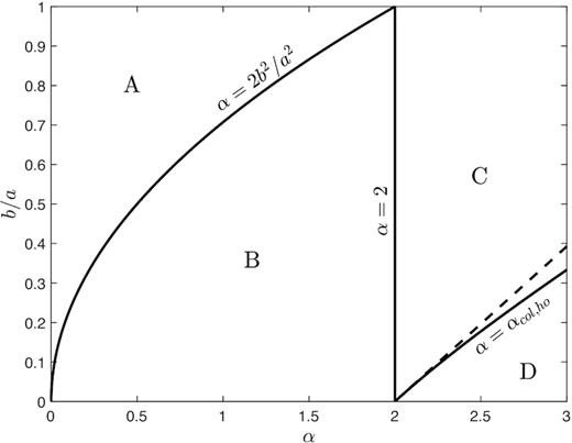
The critical values of α = 2b2/a2 and α = αcol, ho versus b/a for an initially ellipsoidal cocoon. The dashed line shows the approximation for αcol, ho for b/a ≪ 1, as given by equation (D8). The regions labelled A through D are discussed in the text.
