


ABSTRACT
The Southern Photometric Local Universe Survey (S-PLUS) is imaging ∼9300 deg2 of the celestial sphere in 12 optical bands using a dedicated 0.8 m robotic telescope, the T80-South, at the Cerro Tololo Inter-american Observatory, Chile. The telescope is equipped with a 9.2k × 9.2k e2v detector with 10 |$\rm {\mu m}$| pixels, resulting in a field of view of 2 deg2 with a plate scale of 0.55 arcsec pixel−1. The survey consists of four main subfields, which include two non-contiguous fields at high Galactic latitudes (|b| > 30°, 8000 deg2) and two areas of the Galactic Disc and Bulge (for an additional 1300 deg2). S-PLUS uses the Javalambre 12-band magnitude system, which includes the 5 ugriz broad-band filters and 7 narrow-band filters centred on prominent stellar spectral features: the Balmer jump/[OII], Ca H + K, H δ, G band, Mg b triplet, H α, and the Ca triplet. S-PLUS delivers accurate photometric redshifts (δz/(1 + z) = 0.02 or better) for galaxies with r < 19.7 AB mag and z < 0.4, thus producing a 3D map of the local Universe over a volume of more than |$1\, (\mathrm{Gpc}/h)^3$|. The final S-PLUS catalogue will also enable the study of star formation and stellar populations in and around the Milky Way and nearby galaxies, as well as searches for quasars, variable sources, and low-metallicity stars. In this paper we introduce the main characteristics of the survey, illustrated with science verification data highlighting the unique capabilities of S-PLUS. We also present the first public data release of ∼336 deg2 of the Stripe 82 area, in 12 bands, to a limiting magnitude of r = 21, available at datalab.noao.edu/splus.
1 INTRODUCTION
In the past decade, astronomy has firmly shifted towards the collaborative exploration of large observational surveys that provide homogeneous multiwavelength data. In this sense, the Sloan Digital Sky Survey (SDSS; York et al. 2000) opened up a new era of astronomy by covering a large area of the sky at Northern Galactic latitudes with photometry in five broad-band filters, supplemented by an efficient spectroscopic campaign with high completeness for Galactic stars, bright galaxies, and quasars. This has inspired numerous new survey projects in both hemispheres that are extending the SDSS legacy by covering larger areas, observing to greater depths or in other wavelengths.
The Southern Photometric Local Universe Survey (S-PLUS)1 is an imaging survey that will cover ∼9300 deg2 in 12 filters, using a robotic 0.8 m aperture telescope at the Cerro Tololo Interamerican Observatory (CTIO), Chile. Besides the standard optical bands u, g, r, i, and z, filters centred on the following features of stars and nearby galaxies are used: [O ii], Ca H+K, G band, H δ, Mgb, H α, and CaT. As has been shown in Cenarro et al. (2019), this 12-band system is ideally suited for stellar classification, especially for very ([Fe/H] < −2.0) and extremely ([Fe/H] < −3.0) metal-poor stars, and carbon-enhanced metal-poor (CEMP) stars, as well as for a significantly improved photometric redshift estimation of galaxies in the nearby Universe. Although there are many current and future large-area imaging surveys in the Southern hemisphere, S-PLUS provides a unique sampling of the optical spectrum thanks to its seven narrow-band filters. Figs 1 and 2 show comparisons of different optical and near-infrared surveys conducted with telescopes located in the Southern hemisphere, with respect to their area coverage, photometric depth, and number of filters.
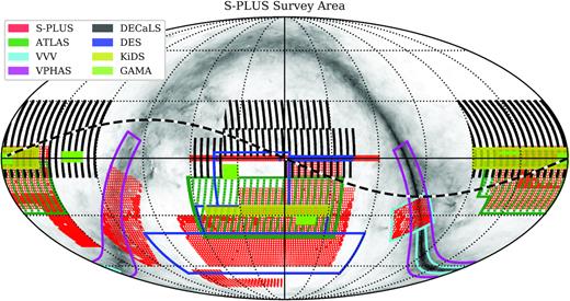
Diagram in equatorial coordinates showing some of the main optical and near-infrared surveys in the Southern hemisphere (we omit the surveys SkyMapper, Gaia, and LSST that cover the entire hemisphere or sky). For the optical surveys: ATLAS (Shanks et al. 2015) is shown in hatched green, VPHAS + is the pink rectangular contour over the Bulge and Disc of the Galaxy, DECaLS is in hatched black, DES (Dark Energy Survey Collaboration 2016) is shown in blue contours, KiDS (de Jong et al. 2015) in filled-yellow, and GAMA in filled-green areas. The only near-infrared survey displayed is VISTA-VVV, in light blue contours, mainly over the Galactic Bulge, overlapping with S-PLUS. The area covered by S-PLUS is shown in red. The dashed black line represents the ecliptic. The background image is the extinction map of Schlegel, Finkbeiner & Davis (1998).
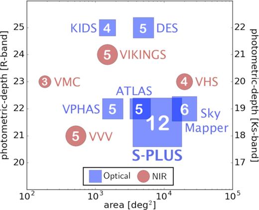
Comparison of several Southern hemisphere optical and near-infrared imaging surveys. The scales on the left and right side of the figure show the approximate depths for the optical surveys (blue boxes) and near-infrared surveys (red circles), respectively, both in AB magnitudes. The number in each box indicates the number of filters in the survey; the box size is proportional to the number of filters.
S-PLUS will also offer synergies with the Gaia mission (Perryman et al. 2001; Gaia Collaboration 2018) that ultimately will deliver (planned for second half of 2021) low-resolution blue and red spectrophotometry for compact sources obtained through prisms, over a similar wavelength range as probed by S-PLUS. Especially in the case of resolved galaxies, the S-PLUS images will be useful for identifying which areas contributed to the Gaia spectra, and what information is being missed. In addition, as pointed out by Cenarro et al. (2019), the Javalambre u band, in combination with the Gaia data, may be useful for improving the Gaia sensitivity at these wavelengths. When the Large Synoptic Survey Telescope (LSST; Ivezic et al. 2008) comes online, it will provide deep observations of the sky observable from CTIO with temporal information, but still using only five broad-band filters. Therefore, it is foreseen that multiband narrow-band surveys using even modest telescopes like S-PLUS can still play a useful role by providing important spectral information that is needed for a wide range of astrophysical applications. Stellar typing and photometric redshifts from multiband surveys such as S-PLUS will provide a valuable resource for cross-checking the calibration of LSST and other surveys.
It is important to note that J-PLUS,2 performed with the T80/JAST telescope in Spain, has been generating data for the last several years. T80-South and its large format camera, including the filters, are a duplicate of that system installed at Cerro Javalambre. Besides doing excellent science (e.g. Cenarro et al. 2019), J-PLUS is also important for calibrating J-PAS, the Javalambre Physics of the Accelerating Universe Survey,3 which will take the narrow-band filter strategy to the extreme, by using 54 equally spaced narrow-band filters (145 Å-wide) and five broad-band filters covering the entire optical spectrum. J-PAS will be performed with a dedicated 2.5 m telescope and a wide field-of-view (FoV) camera at the Javalambre Astrophysical Observatory in Spain (Benitez et al. 2014). However, as of yet, no such survey has been planned for the Southern hemisphere.
This paper describes S-PLUS, highlights its various niches, based on the results from our science verification data obtained during the second semester of 2016 and the second semester of 2018, and presents the first public S-PLUS data release (DR1) in the Stripe 82 region.4 S-PLUS DR1 is available at datalab.noao.edu/splus, and it is characterized in Section 4 and in the NOAO data lab site, as well as in Molino et al. (submitted). Section 2 describes the technical aspects of the survey – the telescope, optics, control system, camera, filter system – and survey strategy, including a description of the five sub-surveys of S-PLUS. Section 3 presents the key science areas of each sub-survey. In Section 4, a brief description of the data reduction pipeline is given. In addition, this section specifies the production of catalogues and data calibration strategies, tests of the point-spread-function (PSF) stability over the images, photometric and photometric redshift depths, and our plans for future data releases (DRs). In Section 5, we present a table with the characteristics of S-PLUS DR1 and describe some preliminary results from the analysis of the first S-PLUS data set. Finally, Section 6 summarizes the paper.
2 THE S-PLUS PROJECT
S-PLUS is carried out with the T80-South (hereafter, T80S), a new 0.826 m telescope optimized for robotic operation; T80S is equipped with a wide FoV camera (2 deg2). The telescope, camera, and filter set are identical to those of the Javalambre Auxiliary Survey Telescope (T80/JAST), installed at the Observatorio Astrofísico de Javalambre (OAJ). T80/JAST is currently performing the Javalambre Photometric Local Universe Survey (J-PLUS), a 12-band survey of a complementary area in the Northern hemisphere (see Cenarro et al. 2019, for details).
2.1 The S-PLUS consortium
The S-PLUS project, including the T80S robotic telescope and the S-PLUS scientific survey, was founded as a partnership between the São Paulo Research Foundation (FAPESP), the Observatório Nacional (ON), the Federal University of Sergipe (UFS), and the Federal University of Santa Catarina (UFSC), with important financial and practical contributions from other collaborating institutes in Brazil, Chile (Universidad de La Serena), and Spain (Centro de Estudios de Física del Cosmos de Aragón, CEFCA). The consortium is open to all scientists from the participating institutes, as well as any other scientist through a vigorous external collaborator program.
2.2 Site
The T80S is located near the summit of Cerro Tololo in central Chile, approximately 200 m north-east of the 4.0 m Blanco telescope. Fig. 3 shows a picture of the telescope and its neighbourhood. T80S sits at an altitude of 2178 m above sea level, at geodetic position (World Geodetic System 84, South latitude and West longitude are negative) −30:10:04.31, −70:48:20.48 (Mamajek 2012). CTIO has highly stable weather conditions, with 82.3 per cent of time used for wide-field survey observations over the period 2013–2016 (S. Heathcote, private communication – note that the last 2 yr included an El Niño cycle). The median total seeing is 0.95 arcsec (FWHM), and the best 10-percentile is 0.64 arcsec (Tokovinin, Baumont & Vasquez 2003).
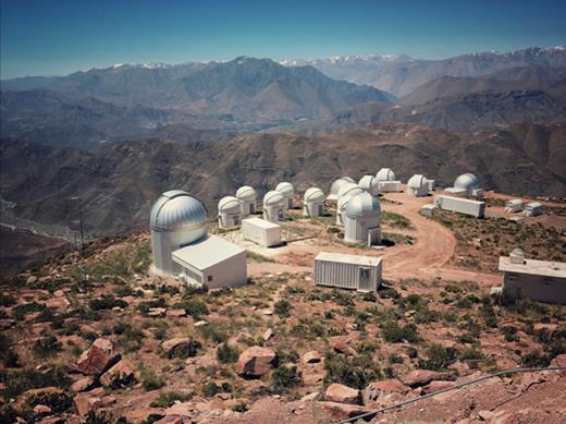
T80S is located on Cerro Tololo, beside the PROMPT telescopes. In this photo, taken in 2017 October, T80S is the largest dome on the left.
2.3 Telescope, optics, and control system
The T80S has a German equatorial mount (model NTM-1000), manufactured by the company ASTELCO,5 under a contract with the company AMOS.6 The optical and telescope designs were done in a close collaboration between CEFCA and AMOS/ASTELCO. The same NTM-1000 universal mount, in EQ configuration, used in T80S, has since then been used in six other telescopes produced by ASTELCO, for the SPECULOOS7 and the SAINT-EX8 projects.
The optical system of T80S consists of a f/4.31 Ritchey–Chretien with one axial Cassegrain focal plane and a clear aperture of 860 mm. This provides a plate scale of 55.56 arcsec mm−1, a total FoV of 130 mm (translating to a 2 deg diameter on the sky), and an optimal FoV of 110 mm (1.7 deg diameter on the sky). The field corrector lens built by AMOS ensures an aberration degradation less than |$1{{\ \rm per\ cent}}$|. A picture of the telescope and its camera is shown in Fig. 4. T80S is housed in an 8 m Ash dome. The telescope can slew between two opposite sky positions in less than 1.5 min, the limiting factor being the time it takes for the dome to move between the two positions. T80S is robotically operated by the chimera9 observatory control system. Developed in python, chimera uses the Pyro3 library to convert the observatory sub-systems into python objects that are accessible over the local network in a distributed way. On top of this framework, a supervisor algorithm takes care of checking the weather conditions, and executes the observations according to constraints imposed by the astronomical conditions.
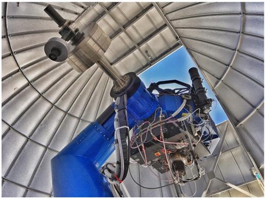
T80S and its wide-field camera.
2.4 Camera
T80S is equipped with an optical imager, T80Cam-S, consisting of a 12-filter system distributed in two filter wheels (see Section 2.5), shutter, entrance window, cryostat, detector, and the corresponding electronics and control system. The camera T80Cam-S is a duplicate of T80Cam (Marín-Franch et al. 2012a); both cameras were produced by the company Spectral Instruments.10 T80Cam-S is operated through the Observatory Control System chimera.
The detector used is a 9232 × 9216 10 |$\mu$|m-pixel array manufactured by the company e2v.11 The telescope plate scale at the detector is 0.55 arcsec pixel−1, and the FoV of the camera is 1.4 × 1.4 deg2. The CCD is read out with 16 amplifiers organized in an 8 × 2 array. During readout of the amplifiers, the camera controller adds 27 pre- and post-scan pixels along the serial direction, and 54 post-scan pixels in the parallel direction for the overscan correction. The detector can be operated at four different readout speeds, and two different gains, with either the 1 × 1 unbinned option or binned 2 × 2. By default, we only use the regular 1 × 1 unbinned option through our control system. See Table 1 for the available readout modes, where the values over all 16 amplifiers have been averaged, for each mode, binning option, and gain. The last column shows the time needed for reading out an entire frame. We regularly use mode 5 for scientific observations since 2017 December, which provides the best compromise between readout speed and readout noise.
Available T80Cam-S readout speed and gain modes.
| Mode | Read rate | Bin | Gain | RON | Time |
|---|---|---|---|---|---|
| (kHz) | (e−/ADU) | (e−) | (s) | ||
| 0 | 1010 | 1 × 1 | 2.03 | 6.60 | 10.83 |
| 1 | 1010 | 1 × 1 | 0.91 | 5.27 | 10.54 |
| 2 | 1010 | 2 × 2 | 1.93 | 6.28 | 6.77 |
| 3 | 1010 | 2 × 2 | 0.89 | 5.15 | 6.78 |
| 4 | 500 | 1 × 1 | 2.12 | 4.47 | 15.97 |
| 5a | 500 | 1 × 1 | 0.95 | 3.43 | 16.57 |
| 6 | 500 | 2 × 2 | 2.02 | 4.25 | 8.14 |
| 7 | 500 | 2 × 2 | 0.93 | 3.34 | 8.13 |
| 8 | 250 | 1 × 1 | 2.15 | 3.49 | 26.60 |
| 9 | 250 | 1 × 1 | 0.96 | 2.74 | 26.60 |
| 10 | 250 | 2 × 2 | 2.04 | 3.33 | 10.80 |
| 11 | 250 | 2 × 2 | 0.94 | 2.69 | 10.81 |
| 12 | 100 | 1 × 1 | 2.15 | 2.79 | 57.69 |
| 13 | 100 | 1 × 1 | 0.96 | 2.34 | 57.69 |
| 14 | 100 | 2 × 2 | 2.05 | 2.67 | 18.58 |
| 15 | 100 | 2 × 2 | 0.94 | 2.32 | 18.58 |
aS-PLUS observing mode since 2017 December.
Fig. 5 illustrates the potential of S-PLUS in probing different astronomical scales. The left-hand panel shows the whole field of a single image, with dimension 1.4 × 1.4 deg2, while the right-hand panels display successive zoom-ins of the same image, including a 15 × 15 arcmin2 field which corresponds to the scale of a nearby group or cluster, a 2 × 2 arcmin2 field representing the scale of a nearby galaxy, and a 12 × 12 arcsec2 field indicating the scale of the bulge of a nearby galaxy.
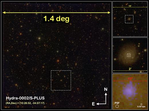
Example of an S-PLUS field, illustrating the potential of combining a very wide FoV telescope with a 9232 × 9216 10 |$\mu$|m-pixel array CCD detector. The large image on the left shows the full S-PLUS FoV. The right-hand panels show consecutive zoom-in images of the centre of the Hydra cluster (15 arcmin on a side, top panel), of one galaxy (2 arcmin on a side, middle panel), and of a galaxy bulge (12 arcsec on a side, bottom panel).
2.5 The S-PLUS filter system
S-PLUS uses the 12-filter photometric system devised for the J-PLUS project. Through a combination of broad- and narrow-band filters that serve to identify the main stellar spectral features (absorption lines and continuum), this photometric system was designed for the optimal classification of stars (Gruel et al. 2012; Marín-Franch et al. 2012b). As illustrated in Fig. 6, the filter system is composed of seven narrow-band filters (J0378, J0395, J0410, J0430, J0515, J0660, J0861) that coincide with, respectively, the [OII], Ca H + K, H δ, G band, Mgb triplet, H α, and Ca triplet features. The system also includes the u, g, r, i, and z broad-band filters which serve to constrain the spectral continuum of sources. The g, r, i, and z bands are similar to those from SDSS (Fukugita et al. 1996), with some small zero-point differences, listed in Table A1. The u-band filter is the Javalambre u-band filter, which has a slightly more efficient transmission compared to the SDSS u band, as described in Cenarro et al. (2019).
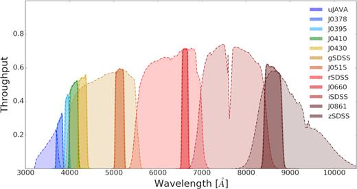
The Javalambre 12-filter system. The y-axis shows the total efficiency of the S-PLUS filters, obtained through the multiplication of the average filter transmission curves, the atmospheric transmission, the CCD efficiency, and the primary mirror reflectivity curves. Different filters are coloured according to the labels shown in the legend at the right.
Fig. 6 presents the total transmission curves of the S-PLUS photometric system. It includes contributions from the filter transmission themselves (measured in CEFCA, in 2015 – available in the project website),12 the atmospheric transmission (Noll at al. 2012), the efficiency of the CCD (as measured by e2v) and the primary mirror reflectivity curve (as measured in CTIO, in 2016 – the curve had no measurements beyond 880 nm; an extrapolation guided by the aluminium reflection curve was applied). The 12 filters are distributed between two filter wheels, which are installed inside T80Cam-S. The 2D filter transmission maps were obtained by performing laboratory measurements over a 10 × 10 evenly spaced grid across the filter surface. Note that curves for the secondary mirror and the corrector were not included in the computation of the total transmission curves shown in Fig. 6. The central wavelengths and full width at half-maximum (FWHM) of the filters+atmosphere+CCD + M1 transmission curves are listed in Table 2.
Summary of S-PLUS filters.
| Filter | λeff | Δλ | Comment |
|---|---|---|---|
| name | (Å) | (Å) | |
| uJAVA | 3563 | 352 | Javalambre u |
| J0378 | 3770 | 151 | |${}[\mathrm{O}\, \rm \small {II}]$| |
| J0395 | 3940 | 103 | Ca H + K |
| J0410 | 4094 | 201 | H δ |
| J0430 | 4292 | 201 | G band |
| gSDSS | 4751 | 1545 | SDSS-like g |
| J0515 | 5133 | 207 | Mgb Triplet |
| rSDSS | 6258 | 1465 | SDSS-like r |
| J0660 | 6614 | 147 | H α |
| iSDSS | 7690 | 1506 | SDSS-like i |
| J0861 | 8611 | 408 | Ca Triplet |
| zSDSS | 8831 | 1182 | SDSS-like z |
Fig. 7 shows examples of spectra of different objects (a quasar, a galaxy, an A0 star, a planetary nebula, and a symbiotic system) convolved with the filters, indicating that the photometric system naturally captures the spectral information in greater detail than the five-band SDSS or the broad-band UBVRI photometric systems.
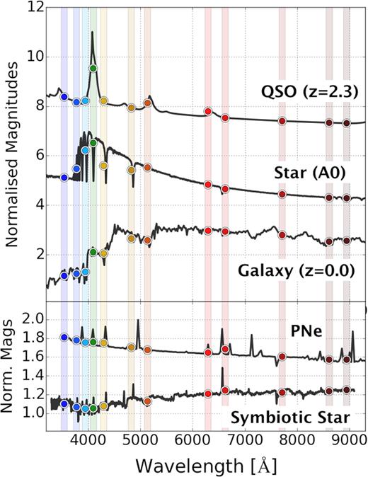
Examples of different spectra (solid black lines) and their convolution with the S-PLUS 12-filter photometric system (coloured dots). From top to bottom: a quasar, a main-sequence star, an early-type galaxy, a planetary nebula, and a symbiotic star. The vertical bands correspond to the effective wavelengths of the S-PLUS filters. The coloured dots indicate the expected magnitudes after convolving the spectra with the S-PLUS filter transmission curves.
2.6 Overview of the S-PLUS scheduling strategies
S-PLUS is composed of five sub-surveys, described in detail in the next section. The robotic operation of the telescope allows autonomous management of the observations of these sub-surveys. The observatory control system (chimera) contains a built-in queue execution module capable of conducting different modes of observations. In standard configuration mode, a set of observations is planned and fed into the queue before the night starts. A separate module automatically selects suitable target fields belonging to the different sub-surveys, given a set of sky conditions and assigned priorities, and feeds them into the queue execution module.
During day-time operations, the module pre-selects suitable target fields and simulates the observing night for different sky conditions. Remote operators check the results of the simulation and, if required, apply corrections to the scheduling parameters. During night-time operations, the module is fed with telemetry on sky and system data, and is able to make scheduling adjustments depending on the conditions.
3 OVERVIEW OF THE S-PLUS
In order to optimize the usefulness of S-PLUS data for the different science topics of interest to the collaboration, the S-PLUS is divided into five sub-surveys, which are detailed in Sections 3.1–3.5 below. Additional information on the sub-survey areas, exposure times, filters, and cadences are summarized in Table 3; their sky coverage is shown in Table 4 and Fig. 8.

Footprint of three of the five S-PLUS sub-surveys, overplotted on to the extinction map of Schlegel et al. (1998) in Cartesian projection. The red squares show the Main and Ultra-Short Surveys, which share the same area. The blue squares show the Galactic fields. The yellow squares highlight the area of the Magellanic Clouds, which are included in the Main Survey. The filled areas have already been observed at the time of this writing, in 2019 March. Magenta is the area of the Stripe 82 contained in DR1 – this is part of the Main Survey but we highlight it with a different colour for clarity.
Overview of the S-PLUS sub-survey strategies.
| Sub-survey | Area | Visits | Filters | Texp | Sky | FWHM | Moon |
|---|---|---|---|---|---|---|---|
| Main Survey | 8000 deg2 | 1 | all | Table 5 | phot | <2.0 arcsec | grey/dark |
| Footprint: | |||||||
| see Fig. 8 | |||||||
| Ultra-Short Survey | 8000 deg2 | 1 | all | 1/12 of MS | non-phot | any | any |
| Variability Fields | TBD | TBD | TBD | TBD | non-phot | any | any |
| Galactic Survey | 1300 deg2 | 1 | all | Table 5 | phot | any | any |
| 1 | r′, i′, H α | 1/12 of MS | non-phot | any | any | ||
| For selected Galactic fields | >25 | r′, i′, H α | Table 5 | non-phot | any | any | |
| Marble Field Survey | Dorado group, M83 | all | Table 5 | phot | >2.0 arcsec | grey/dark | |
| See Table 6 | SMC/47Tuc, Hydra Cluster |
Survey coordinates.
| (RA, Dec.) | |||
|---|---|---|---|
| Galactic Survey | Disc (polygon with vertices) | (136°, −40°); (133°, −60°); (110°, −4°); (92°, −14°) | |
| Bulge (polygon with vertices) | (287°, −26°); (276°, −44°); (268°, −17°); (256°, −34°) | ||
| Main and Short Surveys | Stripe82 | 0° < RA < 60° and 300° < RA < 360° | −1.4° < Dec. < +1.4° |
| Hydra cluster | 150° < RA < 165° | −48° < Dec. < −23.5° | |
| Magellanic Clouds | 65.5° < RA < 98° | −69° < Dec. < −62.5° | |
| 2° < RA < 98° | −75.5° < Dec. < −69° | ||
| Remaining S-PLUS fields | 323.5° < RA < 359.5° | −15.5° < Dec. < −1.4° | |
| 0° < RA < 30° and 315° < RA < 360° | −30° < Dec. < −15.5° | ||
| 0° < RA < 75° and 315° < RA < 360° | −60° < Dec. < −30° | ||
| 150° < RA < 165° | −23° < Dec. < +5° | ||
| 165° < RA < 225° | −26.5° < Dec. < +5° | ||
3.1 The Main Survey
The Main Survey (MS) covers an area of ∼8000 deg2 with a single epoch observation of each field, per filter, under photometric conditions and seeing from 0.8 to 2.0 arcsec. Three consecutive dithered exposures are taken in each filter, for a total exposure time of approximately 1 h and 30 min per field. Each of the three individual exposures of the MS (taken with the exposure times shown in Table 5) are taken at slightly different positions in order to minimize the contribution from bad pixels and to facilitate cosmic ray cleaning. The dither offsets amounts to 10 arcsec along the RA direction (∼18 pixels). In order to mitigate differences in S/N in the edges of the images due to the dithering strategy, we ensure an overlap between images of at least 30 arcsec. This procedure is also useful to produce a homogeneous photometric calibration across the fields.
Main Survey exposure times.
| Filter | Texp |
|---|---|
| name | (s) |
| u | 3 × 227 |
| J0378 | 3 × 220 |
| J0395 | 3 × 118 |
| J0410 | 3 × 59 |
| J0430 | 3 × 57 |
| g | 3 × 33 |
| J0515 | 3 × 61 |
| r | 3 × 40 |
| J0660 | 3 × 290 |
| i | 3 × 46 |
| J0861 | 3 × 80 |
| z | 3 × 56 |
| Filter | Texp |
|---|---|
| name | (s) |
| u | 3 × 227 |
| J0378 | 3 × 220 |
| J0395 | 3 × 118 |
| J0410 | 3 × 59 |
| J0430 | 3 × 57 |
| g | 3 × 33 |
| J0515 | 3 × 61 |
| r | 3 × 40 |
| J0660 | 3 × 290 |
| i | 3 × 46 |
| J0861 | 3 × 80 |
| z | 3 × 56 |
Our MS observing strategy is a modification of the J-PLUS strategy, and it is expected that the data sets from both S-PLUS and J-PLUS can be combined in the future for scientific projects where a large area (∼16 000 deg2) is desirable. The S-PLUS MS strategy is mainly motivated by the requirements set by the extragalactic science. The original goal was to match the photometric depth of SDSS in the broad-band filters; however, S-PLUS images are, on average, shallower than SDSS (see Section 4.6 and Table 8). The MS has significant overlap with Pan-STARRS (Schlafly et al. 2012), DES (Dark Energy Survey Collaboration 2016), KiDS (de Jong et al. 2015), and ATLAS (Shanks et al. 2015), and can thus provide improved photometric redshifts for objects in these fields down to rAB ∼ 20 (see Section 4.7).
The determinations of photo-z, environment indicators, and star–galaxy separation (described in Section 5) using DR1, will form the basis for a number of important extragalactic studies. For example, we expect to detect several million galaxies in the MS – from these data we plan to build a new multiwavelength galaxy catalogue, with uniform environment criteria, choosing from isolated galaxies to groups/clusters. This will extend previous Southern hemisphere catalogues to a complete, volume-limited sample, mitigating projection effects by using the more precise S-PLUS photometric redshift information (δz/(1 + z) = 0.02 or better, see Section 4.7).
Exploring the 12-band filter information, we will be able to recover galaxy morphologies and stellar populations, in order to perform a pixel-by-pixel or region-by-region spectral energy distribution (SED) analysis, in an integral-field-unit approach (IFU-like science). The narrow-band filters used in S-PLUS are tailored to study absorption and emission lines at z = 0. In particular, the filter J0660 is suitable to study H α (λ = 6563 Å) up to redshifts z ≲ 0.015, providing an important tool to measure the star formation rate (SFR) of galaxies in the local Universe.
S-PLUS will also be of fundamental importance for studies in our Galaxy. It will allow searches for streams and substructures not yet known in the Galactic halo. In this respect, blue horizontal-branch (BHB) stars and blue stragglers may be excellent indicators of structure. Based on an extrapolation of the SDSS survey (York et al. 2000), we should be able to detect over 50 000 BHB stars and 100 000 blue stragglers in the MS footprint. Both types of stellar objects are interesting to evaluate the stellar density of the Galactic halo profiles, and their colours may provide valuable information about the age gradient across the halo system of the Milky Way (Santucci et al. 2015; Carollo et al. 2016).
Other important and complementary tracers of the structure of our Galaxy are planetary nebulae and globular clusters. Statistical tools, such as principal component analysis, and classification tree analysis, among others, will help evaluating which combinations of magnitudes and colours work best to identify and study different classes of objects. As an example, colour–colour plots using filters J0515, J0660, and J0861 are a useful selection tool for identifying halo planetary nebulae and symbiotic stars, given their characteristic spectra (see Fig. 9). Furthermore, the 12-band filter system is sensitive to changes in stellar atmospheric parameters, including effective temperature (Teff), surface gravity (|$\log \, g$|), metallicity ([Fe/H]), and abundance ratios such as [C/Fe] and [α/Fe], and appear superior in the determination of stellar parameters compared to the five-band SDSS system (Whitten et al. 2019).

The colour–colour diagram J0515–J0660 versus J0660–J0861, used here to separate halo planetary nebulae (HPNe) and symbiotic stars (SySts). Symbols correspond to different emission line objects: modelled HPNe (dark green stars – seen from the middle to the right of the diagram); observed HPNe (black circles); SDSS quasars with redshift in the range from 1.3 to 1.4 (light-green boxes), 2.4 to 2.6 (blue diamonds), and 3.2 to 3.4 (orange triangles); SDSS cataclysmic variables (CVs, violet circles); SDSS star-forming galaxies (SFGs, cyan triangles); symbiotic stars from Munari & Zwitter (2002) (red boxes, see also the new catalogue of SySts, Akras et al. 2019); symbiotic stars from IPHAS (red triangles) and extragalactic H ii regions (grey diamonds). Note that the halo planetary nebulae (dark green stars and black circles) and symbiotic stars (red boxes and triangles) comprise a fairly well-defined locus (and mostly away from other objects) in this colour–colour diagram, not occupied by any other emission-line objects except for the extragalactic H ii regions (grey diamonds).
Finally, as each MS pointing consists of observations in 12 filters, each having three exposures, we obtain 36 time-steps that could also be used to detect (bright) objects that move or vary in brightness. By alternating observations in blue and red filters, we increase the temporal window in which an object is observed in two or more adjacent narrow bands. This will allow building light curves on time-scales shorter than about 30 min, for many tens of thousands of variable stars. Thus, it is clear that the MS data can be used for a wide range of scientific topics, from Solar system to Cosmology.
3.2 The Ultra-Short Survey
The Ultra-Short Survey (USS) has the same footprint as the MS, with exposure times that are 1/12th of the values shown in Table 5. Therefore, the saturation limit is brighter in all 12 filters (typically 8 mag, instead of the typical 12 mag for the MS). This allows covering an important scientific niche, the search for bright low-metallicity stars.
The most metal-poor stars in the Galactic halo carry important information about the formation and early evolution of the chemistry in the early Universe, as well as in the assembly of the Milky Way. Two subclasses are of great interest:
The ultra metal-poor (UMP; [Fe/H] < −4.0, e.g. Beers & Christlieb 2005; Frebel & Norris 2015) stars, which are believed to be formed by gas clouds polluted by the chemical yields of the very first (Population III) stars (Iwamoto et al. 2005). More than 80 per cent of the observed UMP stars in the Galaxy present enhancements in carbon (e.g. Lee et al. 2013; Placco et al. 2014b), the so-called CEMP stars, and
The highly r-process-element enhanced stars (r-II; with [Fe/H] < −2.0 and [Eu/Fe] > +1.0, Beers & Christlieb 2005), which provide crucial information about the astrophysical site(s) of the rapid neutron-capture process. The production of r-process elements has remained elusive since the seminal work of Burbidge et al. (1957), but recent observations of the electromagnetic counterpart of the first neutron star merger detected by LIGO can possibly provide the final piece of this cosmic chemical puzzle (Abbott et al. 2017; Shappee et al. 2017).
UMP stars are intrinsically rare (Placco et al. 2015, 2016; Yoon et al. 2016), and can only be properly classified spectroscopically. Most UMP stars found to date are faint, which limits the amount of spectroscopic information that can be obtained within reasonable exposures times, even with 8–10 m class telescopes. Previous photometric searches for such stars, using SDSS and the SkyMapper Survey (Wolf et al. 2018), were mostly limited to the use of broad-band photometry. In this context, the narrow-band filters from S-PLUS show a clear improvement in the success rate of identifying low-metallicity stars (Whitten et al. 2019), in addition to reaching a saturation limit similar to SkyMapper, which is considerably brighter than SDSS. Fig. 10 shows the effect of changes in metallicity and carbon abundances, compared with the sensitivity curves of J0395 (panel a) and J0430 (panel c), for selected synthetic spectra of stars with fixed temperatures and surface gravities (Whitten et al. 2019). Panels (b) and (d) show the behaviour of the integrated fluxes along the filter areas. In both cases the narrow-band filters used are capable of successfully capturing the changes in [Fe/H], down to ∼–3.0, and changes in [C/Fe], starting at ∼+0.5.
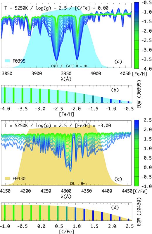
(a) J0395 filter sensitivity curve, compared with synthetic spectra of different metallicities. (b) Behaviour of the integrated flux in the J0395 area for the synthetic spectra shown in (a). (c) J0430 filter sensitivity curve, compared with synthetic spectra of different carbon abundances. (d) Behaviour of the integrated flux in the J0430 area for the synthetic spectra shown in (c).
The 12-band filter system is far more efficient for the identification of these stars. S-PLUS will deliver a catalogue of likely metal-poor stars, suitable for the immediate study of their spatial distributions, which constrains the assembly history of the Milky Way. In this context, given that the candidates from the MS will be fainter than r = 12 mag, due to saturation effects, the S-PLUS USS was devised to find bright low-metallicity star candidates suitable for high-resolution spectroscopic follow-up and studies in the near ultraviolet using the Hubble Space Telescope. Follow-up studies have already been done for a limited number of bright low-metallicity stars (e.g. Placco et al. 2014a, 2015), and additional work is clearly needed to support theoretical studies (Meynet et al. 2010; Nomoto, Kobayashi & Tominaga 2013). Of central importance, S-PLUS USS will then provide targets for subsequent high-resolution spectroscopic studies needed to separate the UMP, CEMP, and r-II subclasses.
3.3 The Variability Fields
The Variability Fields Survey (VFS) will perform repeated observations with a cadence set by the frequency of non-photometric nights, covering a number of fields already observed by the MS. At least 30 per cent of the total time of the survey will be dedicated to the VFS.
Throughout the duration of S-PLUS, the VFS target fields and observing strategies will be set based on calls for proposals for the use of non-photometric nights. This will result in improved detection of each given class of objects, and for the follow-up of targets of opportunity, including cataclysmic variables, eclipsing binaries, variable low-mass stars, asteroids, SNe, AGNs (specially blazars), GRB afterglows, Fermi LAT sources (Acero et al. 2015), and gravitational wave events. We may also identify other transient events, such as the fast radio bursts and tidal disruption events (Burrows et al. 2011).
The VFS data will be inspected for new asteroids and other moving objects. Some SNe may also be identified, although this is not a primary goal of VFS. In addition, the follow-up of Fermi LAT triggers is interesting due to the matching of the typical error box of these triggers (of about 1 deg diameter) to the FoV of the camera. About one third of the sources in the latest Fermi/LAT Source Catalogue (3FGL) are of unknown type (Acero et al. 2015), and their identification may result in a large number of new blazars. Finally, identification and follow-up of the electromagnetic counterparts of gravitational wave events (Abbott et al. 2017) are areas in which VFS may bring important contributions.
At the time of this writing, there is one long-term program that was awarded VFS observing time in 2018B and continuing through 2019, aiming to detect cataclysmic variable stars.
3.4 The Galactic Survey
The Galactic Survey (GS) covers an area of about 1420 deg2 in the Milky Way plane in all 12 filters, including regions of the Bulge (−10° < l < 10° and −15° < b < +5°, for a total of ∼400 deg2) and the Disc (220° < l < 278° and −15° < b < +5°, for a total of ∼1020 deg2, see Fig. 11). The Bulge area, as well as the Disc area within −5° < b < +5°, overlap with VPHAS + in the optical (Drew et al. 2014) and VVV/VVVX in the near-infrared (Minniti et al. 2010).
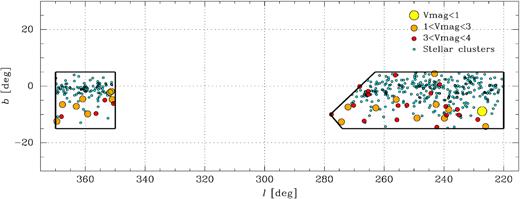
Distribution of stellar open clusters within the S-PLUS GS area, totalling 444 objects from Dias et al. (2002). Stars brighter than V = 4 mag are also marked. The Galactic area is divided in Bulge (large square) and Disc (large pentagon), with a total surveyed area of 1420 deg 2. The region around each V < 4 mag stars is excluded from the observations, reducing the total GS area to 1300 deg2.
The tiling pattern was designed in equatorial coordinates, thus when seen in Galactic projection the tiles are not aligned. The outline of the GS area has a ‘saw-tooth’ profile similar to other Galactic surveys (e.g. VPHAS +). The GS area contains 41 stars brighter than V = 4 mag, the brightest of which is Sirius (α CMa, V = −1.46 mag). Because of saturation problems related to these stars, a total of 62 tiles are excluded from the GS area (reducing the effective area to 1300 deg2).
The first epoch of the GS will have the MS exposure times, followed by two sets of shallower observations (taken with exposure times of duration 1/12th of the MS), only through the r, i, and J0660 filters. Finally, the GS will obtain, for selected fields, at least 25 more epochs in the r, i, and J0660 bands at random cadence over several years, at the same depth as the first-epoch observations (same exposure times as MS). The range of exposure times will probe a wide interval of magnitudes, allowing the sampling of different stellar populations, while observations at different epochs will suit the detection of variable sources, including pulsating RR Lyrae and Cepheids.
In the regions where the extinction is high, the narrow-band colours will break the degeneracy between reddening and spectral type for a large number of stars. Two main studies that are planned with these data are
Variable stars: The cadence and number of observations in the GS is suitable for the detection of variable sources, including pulsating RR Lyrae and Cepheids, CVs and eclipsing binaries, as well as transient sources such as microlensing events. Since the ecliptic crosses the GS Bulge area, asteroids will also be detected in the variability data. Moreover, the narrow-band observations will provide more stringent constraints on the colours of stars undergoing microlensing events and stars harbouring planet candidates, as well as classification of variable sources such as RR Lyrae and CVs. The variability data will be complementary to those obtained by LSST, given that S-PLUS will discover variable stars as bright as g = 9 mag, well below the saturation limit of LSST.
Stellar open clusters: A cross-match between the unprecedented high-precision measurements from the Gaia mission (Perryman et al. 2001; Gaia Collaboration 2018) and the multiband photometry of the S-PLUS survey will allow a systematic study of open clusters down to a magnitude deeper than current analyses. Gaia/DR2 (Gaia Collaboration 2018) will allow a clean determination of cluster membership by applying tools specially designed for this goal (see Sampedro & Alfaro 2016; Sampedro et al. 2017). Taking advantage of the S-PLUS filters will allow us to carry out reliable spectral-type classification for all cluster members, and thus explore the general physical properties of open clusters, such as radius, ages, metallicities, and masses, down to fainter magnitudes.
3.5 Marble Field Survey
The Marble Field Survey (MFS) is composed of a set of specific fields that will be revisited as often as possible under dark or grey nights and photometric conditions, when the seeing is too poor for MS observations, i.e. >2 arcsec. Objects selected for the MFS at the time of this writing are the M83 galaxy, the SMC, the Dorado Group, and the Hydra cluster (see Table 6). The repeated observations of the MFS will increase the depth of the MS images, and is suitable for the study of nearby galaxies, galaxy groups and clusters, and their surroundings, i.e. galaxy haloes, intragroup and intracluster light. The MFS may also be used for identification and characterization of variable sources.
Marble Field Survey.
| Name | RA | Dec. | Obs. | Notes |
|---|---|---|---|---|
| (filter, airmass) | ||||
| M 83 | 13 37 01 | −29 51 57 | Feb–Jun | all, 1.1 |
| SMC | 00 17 47 | −72 13 10 | Jul–Dec | all, 1.4–1.6 |
| (+47 Tuc) | 00 35 33 | −72 13 10 | ||
| 00 53 20 | −72 13 10 | |||
| 01 11 07 | −72 13 10 | |||
| 00 18 57 | −73 27 42 | |||
| 00 37 54 | −73 27 42 | |||
| 00 56 51 | −73 27 42 | |||
| 01 15 47 | −73 27 42 | |||
| Dorado | 04 17 35 | −55 12 10 | Sep–Jan | all, 1.1–1.4 |
| group | 04 17 35 | −55 30 00 | ||
| Hydra | 10 37 54 | −26 41 23 | Jan–May | all, <1.3 |
| cluster | 10 37 10 | −28 04 38 |
4 DATA FLOW, FROM RAW DATA TO SCHEDULED DATA RELEASES
This paper presents the first S-PLUS data release, DR1, on Stripe 82. This section characterizes these data. Further characterization of DR1 is reported in Molino et al. (submitted) and Sampedro et al. (in preparation).
The raw imaging data of S-PLUS are processed daily and data catalogues are generated at the data centre, located in the T80S technical room on Cerro Tololo. Full backups of the raw data are made with LTO6 tapes, for any eventual reprocessing, if needed. The processed data are transferred through fibre connection to IAG/USP, in São Paulo. An overview of the data reduction process is given in Section 4.1.
Multiband photometric catalogues are generated by running the sextractor software (Bertin & Arnouts 1996; Bertin 2010) on a combined reduced image, which is the weighted sum of the reddest (griz) broad-band images. This process is described in Section 4.2.
Photometric calibration of the images is performed with a novel technique using stellar models, as described in detail by Sampedro et al. (in preparation) and in Section 4.3 below. Zero-points are also obtained through standard techniques, by observing typically two spectrophotometric standard stars each night, at three different airmasses. These are also described in the same section.
The astrometric accuracy of the S-PLUS observations and the variation of the FWHM across the fields are investigated in Sections 4.4 and 4.5. The typical photometric depths and photo-z depths of the MS images are derived in Sections 4.6 and 4.7. Information on the data products that will be offered to the community and scheduled data releases is provided in Section 4.8.
4.1 Overview of the data reduction process
The S-PLUS raw data are reduced using an early version (number 0.9.9) of the data processing pipeline jype (developed by CEFCA’s Unit for Processing and Data Archiving, UPAD) designed to reduce data for the J-PLUS and the J-PAS surveys (Cristóbal-Hornillos et al. 2014). This, in turn, is based on the photometric pipeline originally developed for the ALHAMBRA survey (see Cristobal-Hornillos et al. 2009; Benitez et al. 2014; Molino et al. 2014).
The basic reduction strategy consists of four steps: (i) Generating a master bias; (ii) Creating a master flat; (iii) Reducing the individual frames; and (iv) Combining the individual frames into the final astrometrically aligned images. Bias frames are obtained every night, and twilight flats are obtained, whenever the sky is clear, at dawn and at dusk. Twilight flats work well for our purposes. Bias and twilight flat-fields are stable over a period of about a month, and therefore these are obtained for such a period, encompassing the observations of the object. Master flats are obtained for each filter. Only flat fields with counts between 8000 and 45 000 are used. Overscan subtraction, trimming, and bias subtraction is applied to each individual flat-field. Master flats are then created by obtaining, for each pixel, the median value, with 3σ clipping, of all usable flats of a given filter, after scaling each image by its mode. This is performed using the task imcombine of Image Reduction and Analysis Facility iraf13 with options median, sigclip, scale = mode, and zero = none. Finally, the master flats are normalized to have a mean of unity.
The reduction of individual images consists of applying the overscan subtraction, trimming, bias subtraction, and master flat division. Then, cosmetic corrections (removing satellite tracks and cosmic rays) and fringing subtraction are performed. Satellite track and cosmic ray subtraction is performed using either satdetect, in the first case, and lacosmic (van Dokkum 2001) or retina filter in the second case. Fringing frames are obtained by combining the final individual frames that suffer from fringing, usually only in the z filter. The fringing patterns are stable over several months, so a single fringing frame is made by combining all images over such a period that do not have any bright objects. The last step is the combination of the individual images, which is done by obtaining the median, with 3σ clipping, pixel by pixel, for typically three images of each field and filter. This is performed using the task imcombine of iraf with options median, sigclip, scale = none, and zero = mode.
After the final images are produced, data catalogues are generated, as described in the next subsection. The data also need to be calibrated, as described in Section 4.3. After calibration is accomplished, the instrumental magnitudes are replaced by calibrated magnitudes in the final catalogues.
4.2 Deriving multiband photometric catalogues
Deriving accurate multiband photometric catalogues suitable for all of the scientific cases described throughout Section 3 is challenging. It requires an optimized photometric tool, capable of identifying and correcting the specific observational effects that make images inhomogeneous, in particular, the smearing of objects due to variations in the point spread function across bands. This is an effect that, if not taken into account, can cause the photometric apertures to integrate light from different regions of an object.
We have written an additional pipeline code, based on the sextractor software, that analyses the images that come out of the jype pipeline. Photometric catalogues are constructed both in single image mode for individual filters, and in double image mode when performing multiband aperture-matched photometry. The use of a deep detection image is desirable in order to enhance the detectability of faint (or low surface brightness) sources, and to better define the photometric apertures when computing multiband photometry. We automatically generate a detection image for each pointing as a weighted combination of the reddest (griz) broad-band images. This combination makes use of the automatically generated weight maps (produced by the swarp software, Bertin & Arnouts 2010) to account for potential inhomogeneities in the exposure times (i.e. effective depths) across each field, and FWHM differences between bands.
The next steps are the following:
The PSF-corrected photometry is obtained. Initially, the software defines several photometric apertures based on the detection image. Then, for each filter, it estimates how much flux has been missed within that aperture, as a result of the different sizes of the PSF for a single-filter image compared to the detection image. A corresponding correction is then applied, yielding PSF-corrected magnitudes. The full procedure is explained in detail in Molino et al. (2014), in their Section 3.2.
The aperture-matched photometry based on the detection images is obtained. This produces accurate colour determinations for SED-fitting analysis and photometric redshift determinations.
An empirical estimation of the photometric noise in the images is performed, taking into account artificial correlations among pixels (i.e. smoothing) induced during the image-reduction process. The degree of correlation, along with other pieces of information directly related to the sources (such as aperture sizes or integrated fluxes), are used to recompute the noise estimate provided by sextractor. A correction of the photometric uncertainties estimated by sextractor is then applied.
Derivations of photometric upper limits are obtained for sources detected on the detection images and not detected on individual bands. Although there exist several approaches to estimate these photometric upper limits, in S-PLUS we choose to simply convert the integrated enclosed signal within the photometric aperture into a magnitude. These upper limits are of considerable importance for the computation of photometric redshifts.
Weight maps and rms maps are created to minimize the detectability of spurious sources on the detection images.
More details on each of these procedures are given in section 3 of Molino et al. (2014).
4.3 Data calibration and final catalogues
A new photometric calibration technique is employed here, specifically developed for wide-field multiband photometric surveys such as S-PLUS. This complements techniques that are used to calibrate the J-PLUS and J-PAS data (Gruel et al. 2012, López-Sanjuan et al. submitted). The calibration takes advantage of other surveys such as SDSS (Ivezić et al. 2007; Padmanabhan et al. 2008), Pan-STARRS (Schlafly et al. 2012), DES (Burke et al. 2018; Drlica-Wagner et al. 2018) or KiDS (de Jong et al. 2015), which derived photometric calibrations for millions of stars, typically in 4–5 bands, in areas overlapping with S-PLUS. In addition, instead of using complex (and sometimes inaccurate) transformation equations between filter systems, our calibration strategy relies on libraries of stellar models as if they were spectrophotometric standard stars.
As a first step, we select typically 1000 stars in an S-PLUS tile that have known magnitudes from one of the surveys cited above. For each star, a template fitting algorithm is used to find the most likely model that fits the literature photometric information. The stellar templates used are from the Next Generation Spectral Library (NGSL; Heap & Lindler 2007) and the Pickles library (Pickles 1998). The best model is then used to compute a preliminary model stellar magnitude, in each of the 12 bands. The initial zero-points of the S-PLUS filter system are determined through convolution of the filters with the best model, and comparison between the resulting magnitudes and the instrumental magnitudes obtained for each star in the S-PLUS image (obtained with sextractor as described in Section 4.2).
Once the initial zero-point values have been derived for the S-PLUS filter system, the process is iterated by fitting again the stellar models, but now to the newly derived 12-band photometry for each object. After a few iterations, in which the model and instrumental magnitudes are compared, the methodology converges to a final solution for the zero-points in every filter, with typically a few per cent uncertainties. Note that the success of the technique comes from the fact that we are deriving a single number (the zero-point) from the fit to close to 1000 stellar spectra. All zero-points are then absolute calibrated to match Gaia’s photometry (Arenou et al. 2017).
As the calibration strategy is based on the use of stellar libraries, it does not require large campaigns with multiple observations of standard fields. Comparisons were made to the photometry obtained by S-PLUS and SDSS, for the five bands in common (ugriz), with good agreement, as can be seen in Fig. 12. The rms of the distributions for the five filters, ugriz, are 0.06, 0.05, 0.03, 0.05, and 0.03 mag, respectively. Nevertheless, two spectrophotometric stars are observed in three different airmasses every clear night to check the zero-points. Extinction coefficients for the site were obtained using the standard fields observed over 200 nights, for 10 bands (u and z excluded). Average values for the mean atmospheric extinction coefficient obtained for each band are listed in Table 7. Details on the comparisons between the two types of calibrations (standard calibration and using stellar libraries) will be presented in Sampedro et al. (in preparation).
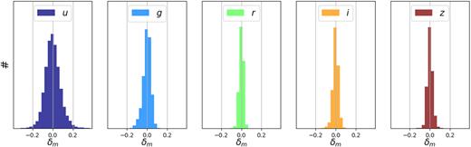
Comparison of S-PLUS and SDSS photometry (δm = magS-PLUS–magSDSS) for objects in DR1 with magnitudes below 20. The rms of the distributions for the five filters, ugriz, are 0.06, 0.05, 0.03, 0.05, and 0.03 mag, respectively, proving the good consistency between the two data sets. The mean differences between the SDSS and the S-PLUS filter systems give an offset in the x-axes of 0.06, −0.02, −0.03, −0.01, and 0.03 mag for the five bands, respectively. This is due to small differences in the filter systems described in Table A1.
Mean atmospheric extinction coefficients obtained from the analysis of standard stars.
| Filter | Extinction coefficient |
|---|---|
| J0378 | 0.414 ± 0.025 |
| J0395 | 0.356 ± 0.011 |
| J0410 | 0.306 ± 0.008 |
| J0430 | 0.268 ± 0.014 |
| gSDSS | 0.188 ± 0.015 |
| J0515 | 0.141 ± 0.013 |
| rSDSS | 0.099 ± 0.005 |
| J0660 | 0.078 ± 0.008 |
| iSDSS | 0.067 ± 0.009 |
| J0861 | 0.035 ± 0.011 |
Once the zero-points are obtained, the final catalogues with calibrated magnitudes are derived. The final data catalogues include the basic astrometric (coordinates), photometric (e.g. fluxes and magnitudes), and morphological (e.g. ellipticity, position angles, major and minor axis ratio, and stellarity) information for all sources detected in the images. Releases of specific Value-Added-Catalogues (VACs) will be made available as part of S-PLUS collaboration science projects. VACs may include photometric redshift measurements, the results of SED-fitting analysis, star/galaxy classification, or other higher order information derived from the S-PLUS images.
4.4 Astrometric accuracy
In this section we describe the level of accuracy reached by our image reduction pipeline. We note that the coordinates computed by the reduction pipeline for DR1, following the ICRS (International Celestial Reference System) and taking the 2MASS catalogue (Cutri et al. 2003) as a reference, are not meant to be used in astrometric investigations per se, but they are useful for locating the great majority of the objects. We have compared the astrometric position of the S-PLUS DR1 sources with those from the SDSS DR12 data on Stripe 82 (Alam et al. 2015) for ∼1M stars in common. To avoid saturated or poorly detected sources, we considered a magnitude interval of 14 < r < 21.
As illustrated in Fig. 13, where the differences between coordinates are represented separately for RA and Dec., we find an average astrometric accuracy of the order of −0.01 and 0.06 pix, respectively, with an rms scatter of 0.34 and 0.24 pixels (0.19 and 0.13 arcsec), respectively. Thus, we assert that our images have been properly corrected, and the coordinates given in our catalogues are robust.
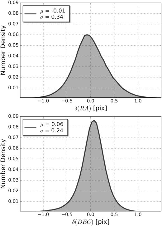
Astrometric accuracy of S-PLUS sources. The two panels show comparisons between SDSS/DR12 and S-PLUS for a common sample of ∼1M stars. A very small mean difference for both RA and Dec. is observed, with a scatter of 0.34 and 0.24 of a pixel, respectively (i.e. 0.19 and 0.13 arcsec, respectively).
4.5 Determination of the stellar FWHM across the field
The S-PLUS DR1 Stripe 82 data were used for checking the average variation of the FWHM of stellar objects across the field. Detection images (i.e. a combination of griz bands) were used for this exercise. The differences in the FWHM measurements for a given star, in the four bands, g, r, i, z, was never more than half a pixel, therefore a simple combination of the four images was appropriate (using only the r band yields very similar results). The FWHM values of typically 500 bright non-saturated stars across each field were measured (using sextractor) and they were normalized to the average FWHM of the bright, isolated, and non-saturated stars in each image. The result is shown in Fig. 14. Note that the average FWHM corresponds to unity, on the scale shown in the right-hand side of the figure, and the variation from the centre to the border is 10 per cent.
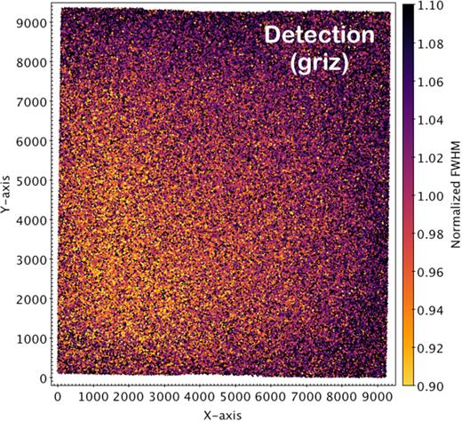
FWHM average variation across images. The figure shows the result obtained using a stack of all images of DR1 in four bands, griz (see Section 4.5 for details). The normalization of the FWHM values for a given field was performed using the average FWHM value derived from a sample of ∼500 bright non-saturated point sources across that field. Note that the variation of the FWHM from the centre of the field to the outskirts is on average 10 per cent.
4.6 Photometric depths
The S-PLUS DR1 Stripe 82 data were used to estimate the average photometric depth of the S-PLUS images. As summarized in Table 8, the photometric depths were calculated using five different definitions for sources detected in a given filter with a signal-to-noise ratio ≥ 3. Here, mpeak corresponds to the Petrosian magnitude at which detections start declining rapidly (i.e. the derivative is zero); |$m_{50{{\ \rm per\ cent}}}$|, |$m_{80{{\ \rm per\ cent}}}$|, and |$m_{95{{\ \rm per\ cent}}}$| correspond to the magnitudes at which it includes 50 per cent, 80 per cent, and 95 per cent of the total detected sources and m3arcs corresponds to the integrated magnitude within circular apertures of 3 arcsec diameter. As can be seen in Fig. 15, where the estimated photometric depths of r- and g-band images at different signal-to-noise ratios are shown, the S-PLUS images are expected to be complete down to a magnitude g < 21.62 and r < 21.38 for all sources (point and extended) with an S/N > 3.
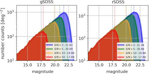
Photometric depths of the S-PLUS g- and r-band images at different signal-to-noise levels, as derived from the S-PLUS DR1 Stripe 82. The dashed lines show the magnitudes for which the samples are considered complete (where the derivatives are zero). As an example, sources with an S/N ∼ 3 are expected to be complete down to a magnitude g < 21.62 and r < 21.38. For sources with other signal-to-noise ratios, the magnitudes of completeness are shown in the legend at the top left.
Photometric depth of images. The table shows the estimated photometric depth of the S-PLUS images using five different definitions, and selecting only sources detected with a minimum signal to noise of S/N ≥ 3 on individual filters: mpeak corresponds to the Petrosian (i.e. total) magnitude at which detections start declining rapidly (i.e. the derivative is zero); |$m_{50\,\mathrm{ per\,cent}}$|, |$m_{80\,\mathrm{ per\,cent}}$|, and |$m_{95\,\mathrm{ per\,cent}}$| correspond to the magnitudes at which it includes 50 per cent, 80 per cent, and 95 per cent of the total detected sources; m3arcs corresponds to the magnitude integrated within circular apertures of 3 arcsec diameter.
| Filter | mpeak | |$m_{50\%}$| | |$m_{80\%}$| | |$m_{95\%}$| | m3arcs |
|---|---|---|---|---|---|
| u | 21.07 | 22.10 | 23.11 | 24.12 | 22.56 |
| J0378 | 20.64 | 21.83 | 22.86 | 23.88 | 22.27 |
| J0395 | 20.11 | 21.47 | 22.52 | 23.65 | 21.87 |
| J0410 | 20.30 | 21.53 | 22.57 | 23.67 | 21.94 |
| J0430 | 20.38 | 21.54 | 22.59 | 23.67 | 21.94 |
| g | 21.79 | 21.88 | 22.85 | 23.88 | 22.16 |
| J0515 | 20.61 | 21.33 | 22.42 | 23.53 | 21.64 |
| r | 21.63 | 21.12 | 22.07 | 22.88 | 21.32 |
| J0660 | 21.36 | 21.02 | 21.98 | 22.93 | 21.12 |
| i | 21.22 | 20.54 | 21.41 | 22.07 | 20.72 |
| J0861 | 20.32 | 20.23 | 21.29 | 22.36 | 20.39 |
| z | 20.64 | 20.27 | 21.05 | 21.77 | 20.37 |
4.7 Photometric redshift depth
S-PLUS DR1 Stripe 82 data were used to characterize the performance of the photo-z estimates for different magnitude and redshift ranges. This data set is ideal because of the availability of a high number of spectroscopic redshifts for galaxies and quasars. For the present exercise, we compiled a sample of galaxies in S-PLUS DR1 Stripe 82, with magnitudes r <21 and redshifts z < 1.0. Our photometric redshift determinations were tested against a sample of galaxies with spectroscopic information taken from the literature. The following datasets were used for constructing our reference sample: SDSS (Abolfathi et al. 2018), 2SLAQ (Richards et al. 2005), 2dF (Colless et al. 2001), 6dF (Jones et al. 2004), DEEP2 (Newman et al. 2013), VVDS (Le Fevre et al. 2005), and PRIMUS (Coil et al. 2011), as well as surveys such as the SDSS- III BOSS (Dawson et al. 2013), SDSS-IV/eBOSS (Albareti et al. 2017), and WiggleZ (Drinkwater et al. 2010). The distributions of blue and red galaxies in this combined sample peak at magnitudes r = 19 and r = 19.6, respectively. The procedure adopted for computing photometric redshift depths of S-PLUS is similar to that explained in Molino et al. (2014) for the ALHAMBRA survey.
Fig. 16 shows the expected fraction of galaxies per magnitude r (left-hand panel) or redshift z bin (right-hand panel) with a maximum photometric redshift error. These values are estimated using the Odds parameter from the bpz code, which allows retrieving samples with a maximum photo-z error. As drawn from the figures, we expect a photo-z precision of δz/(1 + z) = 0.02 or better for 50 per cent of galaxies with a magnitude r ∼ 19.7, or a redshift z < 0.40. Likewise, a precision of δz/(1 + z) = 0.01 or better is expected for 10 per cent of galaxies with a magnitude r < 18.8, or a redshift z < 0.32. About 100 per cent completeness is expected for galaxies with a δz/(1 + z) = 0.03 or better, down to a magnitude r < 20, or a redshift z < 0.5. Similarly, but now in global terms, the same analysis shows that after its completion (i.e. after observing 8000 deg2), the S-PLUS survey will provide photometric redshift estimates for ∼2 million galaxies with a precision of δz/(1 + z) ≤ 0.01, for ∼16 million galaxies with δz/(1 + z) = 0.02, and for ∼32 million galaxies with δz/(1 + z) = 0.025, down to a magnitude r = 21.
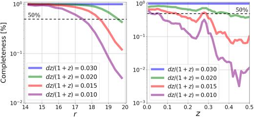
Photometric redshift completeness. The panels represent the expected fraction of galaxies per magnitude r (left-hand panel) or redshift z (right-hand panel) bin with a maximum photometric redshift error. Solid lines correspond to the results obtained from the sample of galaxies in S-PLUS DR1 with spectroscopic redshift information (see text for details). A photo-z precision of δz/(1 + z) = 0.02 or better is expected for 50 per cent of galaxies with a magnitude r ∼ 19.7 or a redshift z < 0.40. Likewise, a precision of δz/(1 + z) = 0.01 or better is expected for 10 per cent of galaxies with a magnitude r < 18.8 or a redshift z < 0.32. The magnitude range of the galaxies on the right-hand panel is the same as for the left-hand panel.
In terms of photo-z precision, the benefit of extending classical five-filter broad-band surveys (such as SDSS; York et al. 2000) can be assessed directly using the S-PLUS data. Molino et al. (submitted) uses the S-PLUS DR1 Stripe 82 data and compare photo-zs obtained with 5 bands with those obtained with 12 bands, using the SED-fitting code bpz (Benítez 2000). As shown in their paper, the 12-band system leads to an improvement in photo-z over the 5-band system of a factor of 4, for galaxies with magnitudes r < 15, a factor of 2.5 for magnitudes 15 < r < 17, and a factor of 1.7 for magnitudes 17 < r < 19. As a function of redshift, the 12-band system leads to a factor of 2 improvement for galaxies with z < 0.1 and of 1.5 for 0.1 < z < 0.4. SDSS-like surveys cannot surpass a certain precision in the photo-z estimates irrespective of the signal to noise of the images. This limitation is imposed by the poorer wavelength resolution provided by the broad-band filters, causing a degeneracy in the colour-redshift space (this actually applies to every survey independent of the filter set).
Note that besides the overall improvement in the photo-z estimates at all redshifts, the S-PLUS filter system provides a special redshift window at which the photo-z estimates undergo a significant improvement (see the right-hand panel of Fig. 16). At the redshift interval z ∼ 0.26–0.32, the [OIII] line (λ = 5007 Å) enters the J0660 filter and the H α line (λ = 6600 Å) enters J0861, improving the photo-z precision.
4.8 Data releases
The public DRs will be primarily hosted by NOAO data lab14 and the Brazilian Virtual Observatory (BRAVO) server at Laboratório de Astroinformática, IAG/USP, in São Paulo.15 The DRs include multiband images, single-mode and dual-mode photometric catalogues, and value added catalogues produced by the consortium. Raw images or intermediate-step reduction products (e.g. weight maps or segmentation images) may be made available upon request. The data will also be accessible through the S-PLUS data portal16 and through queries using the International Virtual Observatory Alliance (IVOA)17 interoperability standards Cone Search, SIA, TAP, and SSAP (Plante et al. 2008; Dowler, Rixon & Tody 2010; Tody et al. 2012; Dowler, Bonnarel & Tody 2015).
The baseline survey plan foresees a 5-yr period to complete the survey. We intend to have six data releases, starting ∼24 months after the start of operations (in 2017 August). The release of S-PLUS data on fields coinciding with the SDSS Stripe 82 region, DR1, accompanies this paper.18 The next DRs are then scheduled for approximately the month of October in five consecutive years starting in 2020.
5 RESULTS FROM THE SCIENCE VERIFICATION DATA
This section first summarizes some key features of the S-PLUS DR1 in Table 9. DR1 is composed of 170 contiguous pointings, adding up to ∼336 deg2 of the Stripe 82 area, observed in 12 filters. The main characteristics of DR1 including a description of the reduction and calibration methods used, an analysis of the spatial distribution of the PSF along the images, as well as the photometric and photo-z depths attained in the DR1 data set, have been described in Section 4.
Summary of DR1 characteristics – Stripe 82 area.
| S-PLUS DR1 data | |
|---|---|
| Area covered | ∼336 deg2 |
| Bands | Broad: u, g, r, i, z |
| Narrow: J0378, J0395, J0410, | |
| J0430, J0515, J0660, J0861 | |
| Number of sources | ∼3 M |
| Number of tiles | 170 |
| Astrometric accuracy | 0.25 pix (0.14 arcsec) |
| Depth (S/N > 3, r band) | 21.38 mag |
| Zero-point accuracy | 1 per cent–2 per cent |
| Seeing | ∼1.5 arcsec |
As described in Section 3.1, files from the MS are generally dithered by 10 arcsec along the RA direction. However, in the case of the fields of Stripe 82 in the DR1, only those fields observed in 2018 were dithered, the ones in 2016 were not. DR1 fields had no overlapping area. These were decisions made early in the project that were then changed (to include dithering and overlapping areas for the remaining of the survey).
S-PLUS DR1 contains about 3M sources, 2/3 are point-like and 1/3 extended sources. From the sources classified as galaxies, nearly 35 per cent are classified as early/quiescent galaxies and 65 per cent as late/star-forming galaxies. In absolute numbers, S-PLUS DR1 includes ∼350k early and ∼650k late-type galaxies. S-PLUS DR1 catalogues released with this paper have a magnitude cut of r = 21 mag.
This section also presents preliminary results obtained using DR1, which will be detailed in future papers. MS data on Stripe 82 are used to exemplify the usefulness of S-PLUS at improving star/galaxy classification (Section 5.1), at the determination of galaxy cluster/group membership (Section 5.2), in deriving environment density indicators (Section 5.3), in quasar searches (Section 5.4), in morphological studies (Section 5.5), and for IFU-like science projects (Section 5.6).
5.1 Star/galaxy separation applied to the Stripe 82 field
The separation between stars and galaxies is a crucial step for every photometric survey. In the last decades there have been many solutions proposed to deal with this classification issue. Here, a new approach, specifically for multicolour surveys, is presented.
In the experiment described here, the Random Forest technique (Breiman 2001) was used, combining the S-PLUS photometric and morphological information (ellipticity, concentration, and FWHM) to classify objects into stars or galaxies. A matched sample between S-PLUS DR1 Stripe 82 data and the photometric SDSS Stripe 82 catalogue (Jiang et al. 2014 – the latter is complete to ∼r = 24.6) provided reliable classifications for ∼200k objects. This matched sample was used to properly train the Random Forest algorithm. The inclusion of the morphological parameters in the input set of features was crucial for improving the performance of the S-PLUS star/galaxy classifier. The overall performance of the code indicated that 95.7 per cent of the objects are correctly classified down to r = 21. This assumes SDSS photometric classification as a truth table down to r = 21, which is reasonable, given that the magnitude limit of the SDSS sample is ∼r = 24.6, more than 3 mag deeper than S-PLUS. Fig. 17 shows colour–colour diagrams, (g − r) versus (r − i), for galaxies and stars, as classified by SDSS and S-PLUS, to r = 19. Down to this magnitude limit, S-PLUS gets the correct classification for the sources in 97.9 per cent of the cases. We conclude that the star/galaxy classification employed in S-PLUS is able to classify objects correctly, and recovers the stellar and galactic loci in the colour–colour diagrams expected based on the SDSS classification. For further details see Costa-Duarte et al. (submitted).
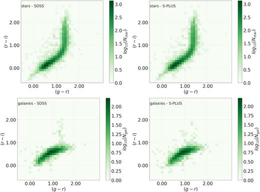
The colour–colour diagram (g − r) versus (r − i) using S-PLUS magnitudes down to r = 19. The overall performance of the code indicates that 97.9 per cent of the objects are correctly classified down to this magnitude limit (see Section 5.1). Upper panels: The stellar locus of objects classified as stars based on SDSS (left) and S-PLUS (right) data. Lower panel: The galaxy locus in the same diagram using the SDSS and S-PLUS classifications.
5.2 Determining group and cluster membership with accurate photometric redshifts
Photometric redshifts (photo-z) have become an essential tool in astronomy, since they represent a quick and inexpensive (in terms of observing time) way of retrieving redshift estimates for a large number of galaxies. Photo-zs are among the primary deliverables of S-PLUS, given that the 12-band photometric system allows higher photo-z precision compared to those derived with, for example, SDSS data, as shown in Molino et al. (submitted). The high quality of the S-PLUS photometric redshifts will enable detailed studies of large-scale structure and galaxy evolution over the entire ∼8000 deg2 area of the MS.
In contrast with areas of the Northern hemisphere covered by SDSS, where all galaxies with r < 17.7 have an observed spectrum, the areas covered by S-PLUS typically do not have an abundance of easy-to-access fully reduced SDSS-like spectra, even if partial areas have been surveyed spectroscopically with other Southern hemisphere telescopes. The new generation of redshift surveys utilizing multifilter photometric systems can play an important role in mitigating this North/South imbalance. Classical 3–4 per cent photometric redshift errors, computed from standard 4–5 broad-band filter systems, can be dramatically diminished to the 1–2 per cent level by simply including narrow-band filters (see Fig. 16). Improved photometric redshift estimates also lead to narrower (i.e. less uncertain) probability distribution function (PDFs) needed for robust statistical analysis. In particular, accurate PDFs can play a key role in the identification of groups and galaxy clusters from photometric data (e.g. Molino et al. 2019). In this regard, the S-PLUS will be used to construct the most accurate photo-z nearby-galaxy catalogue yet produced over a large area of the Southern sky.
In order to illustrate this statement, we selected a galaxy cluster within the Stripe 82 at a redshift z = 0.05, and picked six random early-type galaxies with different apparent magnitudes. Based on the S-PLUS photometry, we computed their photometric redshifts, estimating the most likely redshift and spectral type as well as their PDFs. In Fig. 18 we present a zoom-in of the cluster core in the central region surrounded by six stamps, where in each stamp different coloured points correspond to the observed S-PLUS magnitudes and the solid grey lines correspond to the most likely galaxy templates from bpz. The inner panels in these stamps show the corresponding redshift PDFs computed by the bpz code for each galaxy compared to the cluster redshift (dashed-red vertical line), proving the capability of the S-PLUS data in detecting galaxies with similar redshifts; i.e. groups and galaxy clusters.
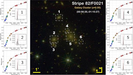
Membership analysis in a cluster of galaxies. The figure shows an example of the typical SED-fitting and photo-z analyses for a sample of six early-type galaxies within a galaxy cluster at redshift z = 0.05. Coloured points in the six stamps around the main figure correspond to the observed S-PLUS magnitudes, and the solid-grey line to the most likely galaxy template. The inner-panels in the stamps show the corresponding redshift probability distribution function (PDF) computed by bpz (grey curve) compared to the cluster redshift (dashed-red vertical line). Note the sharp PDFs, indicating precise photo-z determinations for the brightest cluster members, allowing the identification of galaxies at the same redshift.
The high precision of S-PLUS photometric redshifts (see Fig. 16) of ∼1.5 per cent (2 per cent) for a significant number of galaxies with r < 18.5 (19.7) will allow membership analysis in existing clusters and groups of galaxies down to intermediate magnitudes and redshifts, complementing already existing spectroscopic samples in the Southern hemisphere. At least parts of some important nearby superclusters are in the MS footprint, such as Hydra-Centaurus, Pisces-Cetus, Phoenix, and Horologium. On the other hand, searches in the MS for new structures using techniques that can take advantage of the photometric redshift probability distributions will deliver new catalogues of clusters and groups of galaxies. This will then produce a 3D map of the local Universe over a volume of more than |$1\, h^{-3}$| Gpc3. While the photometric redshift accuracy will not be sufficient for estimating dynamical masses of such systems, masses can be derived for systems in common with those selected in X-ray surveys or in surveys done using the Sunyaev–Zel’dovich effect, or by establishing relations between mass and optical richness or luminosity.
5.3 Galaxy environment and large-scale structure
The environment of a galaxy plays an important role in the current galaxy evolution scenario (Balogh et al. 2004; Blanton & Moustakas 2009; Peng et al. 2010). Several environmental processes are proposed as being responsible for galaxy quenching, such as ram pressure stripping (Gunn & Gott 1972), galaxy mergers (Mihos & Hernquist 1994), and galaxy harassment (Moore et al. 1996). However, all these physical mechanisms act on different scales and in different environments, and their exact relative contributions to the general galaxy evolution scenario have been difficult to establish. The MS will provide accurate photometric redshifts and sufficiently large sky areas, suitable for characterizing galaxy environments in the local Universe. This will allow us to probe the connections between structure formation and galaxy formation, and thus constrain popular approaches such as the halo model (Cooray & Sheth 2002), halo occupation distribution (Berlind & Weinberg 2002; Zehavi et al. 2005), and halo abundance matching (Trujillo-Gomez et al. 2011).
In the following, we show how MS data will be able to constrain the local density contrast of galaxies using a promising tool, the k-NN (k-Nearest Neighbour) technique, adapted to take into account the photo-z uncertainties in our calculations (as also done for the KiDS survey, de Jong et al. 2015). As shown by Costa-Duarte et al. (2018), the relation between galaxy luminosities, density contrasts, and galaxy colours is recovered when applying this technique to photometric redshift data (see their fig. 5).
In order to show the potential of the S-PLUS filter system in retrieving parameters indicative of galaxy environment, we constructed a mock catalogue of S-PLUS, which mimicked the predicted S-PLUS photometric depth and redshift uncertainties. A mock volume-limited sample was generated, including galaxies up to z = 0.25 and Mr < −19.5 + 5log h. The local density of galaxies was then calculated using the approach of Costa-Duarte et al. (2018). The comparison between the density contrasts (|$1 + \delta = \frac{\rho }{\bar{\rho }}$| and k = 5) in spectroscopic and photometric redshift spaces is shown in Fig. 19, presenting a Spearman correlation coefficient of rs = 0.46, and a probability of the null hypothesis p(H0) < 10−3. This exercise confirms that this technique is able to recover the galaxy environment, as measured by local densities, in photometric surveys, in particular using S-PLUS.
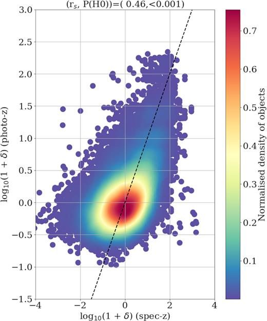
The local density contrasts of galaxies in spectroscopic and photometric redshift spaces. These have been calculated using an S-PLUS mock volume-limited sample (z < 0.25 and Mr < −19.5 + 5log h). The Spearman correlation coefficient (shown at the top) shows a significant correlation between both density contrasts, indicating that we can reliably recover the galaxy environment with S-PLUS photo-zs.
5.4 Searches for quasars
Searches using the SDSS and WISE have provided the largest and most reliable quasar catalogues yet compiled. Wu et al. (2012) first presented the criterion z − W1 > 0.66 (gSDSS − zSDSS) + 2.01 to separate stars and quasars using SDSS and WISE bands, recovering 98.6 per cent of 3089 quasars with redshifts less than 4. For quasars with redshifts lower than 3.2, they suggested a criterion that only depended on WISE bands: W1 − W2 > 0.57. Pâris et al. (2018) made use of W1 and W2 WISE bands along with SDSS bands to identify quasar candidates, resulting in the most recent SDSS catalogue containing 526 356 quasars. Several other authors have also used WISE bands to separate quasars from stars, in particular to increase the numbers of quasars at the bright end of the luminosity function (e.g. Schindler et al. 2017; Yang et al. 2017; Guo et al. 2018). Earlier works based on the COMBO-17 survey had already discussed direct detection of emission lines in quasars through narrow-band optical SED (e.g. Wolf et al. 2001, 2003, 2004). The work described briefly in this section (and further presented in subsequent papers) will complement these previous works.
At specific redshifts, the broad emission lines of quasars can be resolved spectrally by several narrow-band filters of S-PLUS. The best lines to be used for z > 1 quasar detection can be clearly seen in Fig. 20. The C iii line (λ = 1908 Å) passes through the H α filter at z ∼ 1.4. The CIV and Ly α lines become detectable in the bluest narrow-band filter, at z ∼ 1.0 and z ∼ 2.0, respectively. Therefore, S-PLUS will be able to identify quasars, not only through standard UV dropout selection and colour cuts (e.g. Bovy et al. 2011), but also through the direct detection of emission lines (e.g. Abramo et al. 2012; Chaves-Montero et al. 2017). The combination of both broad- and narrow-band filters alone, as well as in combination with WISE bands, will thus allow us to construct a large sample of quasars in the Southern hemisphere, many of which will have accurate photometric redshifts and spectral information from the S-PLUS data alone. Moreover, once the photometric redshifts are known, one can make an estimate of the equivalent widths of the lines that lie within the narrow-band filters.
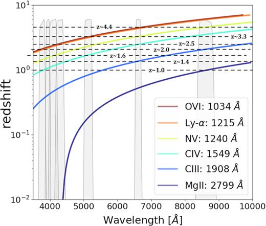
The redshift of typical quasar emission lines as a function of the rest-frame wavelength. This figure summarizes the potential usefulness of S-PLUS magnitudes in the detection and redshift determination of quasars. The transmission curves of the 12-filter system used by S-PLUS are indicated. Several quasar lines are detected by different filters, depending on the quasar redshifts. For example, the Ly α line becomes detectable in the first blue filter of S-PLUS at z ∼ 2.0 and at the J0515 filter at z ∼ 3.3. The S-PLUS narrow-band filters will allow the simultaneous detection of two emission lines from QSOs in at least 7 redshift windows up to a redshift z < 5. This sensitivity may increase the QSO detectability and redshift computation.
In this section, we present some preliminary results on quasar searches using S-PLUS DR1 combined with WISE photometry and using S-PLUS DR1 alone.
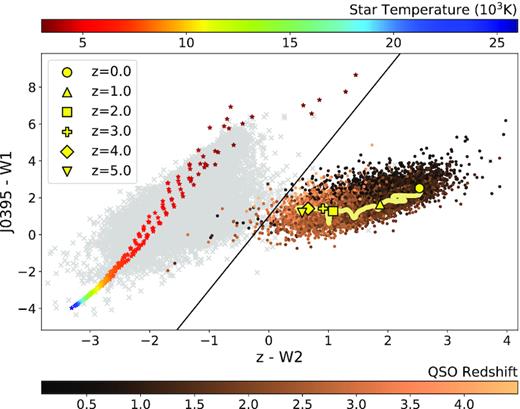
S-PLUS/WISE colour–colour diagram of stars and quasars in the Stripe 82 area from Nakazono et al. (in preparation). Stars with reliable classification in S-PLUS are shown as grey Xs, whereas confirmed quasars (with known spectroscopy) are indicated by circles whose colours depend on the redshift, indicated on the bottom colour bar. Stellar models for different effective temperatures are indicated by star symbols, coloured according to the scale on the top. The yellow curve represents the evolution of the simulated colours for a QSO template with redshift. On top of the curve, the yellow symbols mark the integer values of redshift. The dashed-black line represents an empirical relation (equation 1) to separate stars from quasars. A total of 99.5 per cent of the known quasars in Stripe 82 occupies the expected region in the figure (to the right of the dashed black line), confirming the efficiency of the method.
In Queiroz et al. (in preparation) we perform the object classification without any near-infrared data by employing a machine learning technique, which provides the probabilities that any given point-like source detected with S-PLUS is a quasar, a star, or a galaxy. The method implements a Random Forest algorithm using a training set for each type of object, containing synthetic fluxes with the same level of noise as in S-PLUS, constructed from SDSS-DR12 spectra. Our training sets contain main-sequence stars and white dwarfs, quasars in the redshift range 0.0 < z < 4.0, as well as red and blue galaxies.
The performance of this technique was tested in a sample of about 40k point-like sources detected in S-PLUS DR1 of Stripe 82, again using the star/galaxy classification described in Section 5.1. By applying probability cuts on a magnitude-limited sample (r < 20.5), we reach a completeness of |$76{{\ \rm per\ cent}}$| and a purity of |$\sim 94{{\ \rm per\ cent}}$| for the quasars (of which 1.6 per cent are stars, and 4.2 per cent are galaxies). The purity of the sample with different magnitude cuts is shown in Fig. 22 – note that for r < 18 no stars are classified as quasars. Extrapolating these results to the MS we forecast a total number of approximately 703 000 quasars in S-PLUS brighter than r = 20.5, with |$\sim 94{{\ \rm per\ cent}}$| purity.
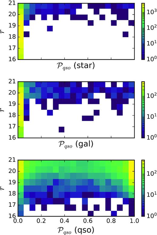
Number of S-PLUS quasars detected in the Stripe 82 that are classified as stars (upper panel), galaxies (middle panel), and quasars (bottom).
We also estimate the photometric redshift probability distribution for the point-like sources classified as quasars. The method devised finds the best fit to the S-PLUS data using a linear combination of quasar eigenspectra derived from a principal component analysis (Yip et al. 2004; Abramo et al. 2012) plus an attenuation law. We also test the performance of our photo-z code on the spectroscopic sample of point-like sources, by computing the photo-z precision |$\sigma _{z} = \mathsf {med}|z_{\mathrm{ photo}}-z_{\mathrm{ spec}}|/(1+z_{\mathrm{ spec}})$|. For the magnitude-limited samples r < 20.5, r < 19.0, and r < 18.0 we obtain, respectively, σz = (0.0655, 0.0545, 0.0220).
5.5 Determination of morphological parameters
S-PLUS will provide a large sample of nearby galaxies for morphological studies and SED analyses. We will use MS data to perform parametric (e.g. Vika et al. 2015) and non-parametric (Ferrari, de Carvalho & Trevisan 2015) multiband morphological analyses. Although measurements of the Sérsic index and effective radius as a function of wavelength can be used to perform an automated and robust classification of galaxies (Vika et al. 2015), Ferrari et al. (2015) show that the non-parametric code morfometryka is ideal to distinguish between elliptical and spiral classes with a mismatch between classes smaller than 10 per cent. Combining parametric and non-parametric approaches we will be able to classify all well-resolved MS galaxies. SED-fitting codes will be used to extract stellar population parameters, attenuations, and stellar masses from the observed SEDs (e.g. Díaz-García et al. 2015; Magris et al. 2015; Mejía-Narváez et al. 2017). When combined with the accurate photometric redshifts, the morphology measurements, spectral energy distribution modelling, and estimates of the environments will produce a very rich data set for studying galaxy evolution.
In this section, we present preliminary results obtained by applying the codes morfometryka (Ferrari et al. 2015) and megamorph (Bamford et al. 2011) to an image of a bright spiral galaxy in Stripe 82, NGC 0450, and its companion, using data from DR1, to provide an example of what is planned for the entire survey. morfometryka does not require any initial input for the fit, except that the galaxy must be roughly centred on the image stamp and an image of the PSF must be available (Ferrari et al. 2015). The program estimates the sky background iteratively, segments the image, performs basic photometry, and measures morphometric parameters. One example of a typical output from morfometryka (fully explained in Ferrari et al. 2015) is shown in the top panel of Fig. 23. These include single Sérsic 1D and 2D fit parameters and non-parametric morphometric parameters (concentration, asymmetry, clumpiness, Gini, the second moment of the light distribution, entropy, spirality, and light-profile curvature). These parameters can be combined to assign a morphological class to each galaxy, or they can be used to yield information about the structure of the galaxy. For example, the concentration varies critically among different galaxy classes; the polar map, used to compute the image gradient and σψ, has a nearly flat profile for ellipticals, whereas for spiral galaxies it exhibits peaks corresponding to the spiral arms, and in S0 galaxies it may have some variation due, for example, to the presence of a bar. Subsequently, one uses the morfometryka outputs to create the initial input file to run megamorph-galfitm. In Fig. 23, bottom panel, upper row, we show the images of the galaxy in 12 bands, and in the middle row, we show the models obtained fitting all bands simultaneously using megamorph-galfitm. The galaxy has been fitted with two components, a disc (exponential profile) and a bulge (Sérsic profile). The residuals are shown in the third row. Considering these results, exemplified in only one case here, we plan to devise a galaxy morphological classification method, based on the derived parameters and best-fitting models.

Upper panel:morfometryka (top, from left to right): Original image; 2D Sérsic model image; the residual between image and model; asymmetry map used to compute A1; and smoothness map used to compute S1. Bottom: Various measurements (see text for details); Brightness profile (arbitrary units) and model fits; polar map used to compute image gradients and σψ; brightness profile curvature. Lower panel:megamorph-galfitm: First row – galaxy images in the 12 S-PLUS bands (u, J0378, J0395, J0410, J0430, g, J0515, r, J0660, i, J0861, and z, respectively); second row – galaxy models as fitted with galfitm; third row – residuals. The colour bar shows relative intensity measurements with darkest colours indicating largest fluxes.
5.6 Example of IFU-like science with S-PLUS
S-PLUS will provide large FoV observations, similar to low-resolution integral field spectroscopy, for thousands of nearby galaxies, whose stellar populations are of great interest for galaxy formation and evolution studies. An important goal of S-PLUS is to explore this capability to determine accurate stellar population parameters, such as ages, metallicities, and possibly their radial gradients for extended sources, overcoming known problems such as the age–metallicity degeneracy (Worthey 1994), which complicates the differentiation of stellar populations when only optical colours are used. In particular, San Roman et al. (2019) have shown that stellar populations derived with the 12-band Javalambre photometric system are very dependent on the choice of models and methods.
In this context, we developed a novel method to derive stellar populations for multiband photometric surveys in general (Barbosa et al., in preparation), which we apply to S-PLUS. The main idea is to use a hierarchical Bayesian method that allows the modelling of all locations inside a galaxy simultaneously, such that a consistent modelling for the whole galaxy is obtained without completely erasing the information of the gradients. To test the new method, we have been using galaxies in the Stripe 82 region also observed by the CALIFA survey (Sánchez et al. 2012), whose stellar population were made available by de Amorim et al. (2017). Fig. 24 shows the results of the attenuation and stellar population gradients for NGC 429 using our method in comparison with those observed by de Amorim et al. (2017). However, given that we have been using single stellar population models from Vazdekis et al. (2010), which have a larger metallicity coverage than de Amorim et al. (2017), we have also determined ages and metallicities of the CALIFA galaxies independently, using the ppxf code (Cappellari 2017). The good agreement of attenuations, ages, and metallicities of our photometric observations with spectroscopic results, in particular when the same single stellar population models are adopted, indicates that we are able to properly constrain the stellar populations using S-PLUS data, allowing a better census of the metallicities and ages in the local Universe.
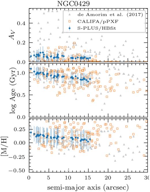
Comparison of the radial profile of the attenuation (top), mass-weighted ages (middle), and metallicity (bottom) of NGC 429, one of the galaxies in the STRIPE 82 also observed by CALIFA. The blue circles indicate the results obtained with our new hierarchical Bayesian methods using S-PLUS data, whereas orange squares indicate the results of the CALIFA data cubes using ppxf, both using the same stellar population models from Vazdekis et al. (2010). Grey triangles indicate the results made available by de Amorim et al. (2017) using CALIFA data and a slightly different version of the stellar population models.
6 SUMMARY
T80S is a 0.8m robotic telescope with a wide-field camera (2 deg2) that uses five broad- and seven narrow-band filters placed over the main spectral features of stars and galaxies. Its first main goal is to conduct S-PLUS, started in 2017 August and expected to reach completion in 5 yr. The main characteristics of the telescope and the survey are summarized in the following.
S-PLUS is a 12-band optical survey aiming at imaging ∼8000 deg2 of the sky at high Galactic latitudes and ∼1300 deg2 over the Disc and Bulge of our Galaxy. It complements a twin project in the Northern hemisphere, J-PLUS, being carried out with the T80/JAST, located at Cerro Javalambre, Spain.
The combination of a wide FoV telescope + camera and a 12-band filter set will allow the study of a large number of scientific topics, from Solar system to Cosmology.
The first public data of S-PLUS have been released together with this paper. These comprise 170 fields that cover about ∼336 deg2 of Stripe 82, in 12 bands. The data reach a depth of r ∼ 21 AB mag in the broad-bands and r ∼ 20.5 AB in the narrow-band filters, for sources detected with a significance larger than S/N > 3. The bright saturation limit of the data is r ∼ 12. The data are available at NOAO data lab.
The typical photo-z precision derived from S-PLUS, especially for galaxies with r < 20.0, surpasses that of other overlapping photometric surveys, making it possible to revisit membership analyses of nearby groups and clusters of galaxies. We forecast that, after imaging ∼8000 deg2 of the sky, a total of ∼2 million, ∼16 million, and ∼32 million galaxies will be measured in the S-PLUS survey with photo-z precisions of σz < 1.0 per cent, σz < 2.0 per cent, and σz < 2.5 per cent, respectively.
Some of the main niches of S-PLUS, highlighted in this paper, are: (1) Mapping the nearby Universe, (2) Performing a pixel-by-pixel SED analysis (i.e. IFU-like science) of resolved nearby galaxies to study stellar populations, gas and dust, (3) Finding metal-poor and carbon-enhanced metal-poor stars, and (4) Identifying large numbers of new quasars with precise redshifts.
For all the science examples given in this paper, the tools developed for S-PLUS will ultimately be used for J-PAS, using deeper data and more precise photo-zs, given that J-PAS has 54 narrow-band and 5 broad-band filters.
S-PLUS also provides a rich laboratory for extension efforts. Examples could include teaching and hands-on science projects using S-PLUS data in schools, presentations to community organizations, individual studies such as citizen science efforts, offering educational content via interactive Web sites, or simply engaging the public through social media. S-PLUS, thus, offers a great toolbox to engage young students in STEM (Science, Technology, Engineering, Mathematics) and natural sciences.
Beyond S-PLUS, the plan is to use T80S as a dedicated telescope specifically to do survey-like projects, targeted at a variety of science cases that could be useful for a large number of astronomers from the involved communities.
ACKNOWLEDGEMENTS
The S-PLUS project, including the T80S robotic telescope and the S-PLUS scientific survey, was founded as a partnership between the Fundação de Amparo à Pesquisa do Estado de São Paulo (FAPESP), the Observatório Nacional (ON), the Federal University of Sergipe (UFS), and the Federal University of Santa Catarina (UFSC), with important financial and practical contributions from other collaborating institutes in Brazil, Chile (Universidad de La Serena), and Spain (Centro de Estudios de Física del Cosmos de Aragón, CEFCA). The members of the collaboration are grateful for the support received from the Conselho Nacional de Desenvolvimento Científico e Tecnológico (CNPq; grants 312333/2014-5, 306968/2014-2, 142436/2014-3, 459553/2014-3, 400738/2014-7, 302037/2015-2, 312307/2015-2, 300336/2016-0, 304184/2016-0, 304971/2016-2, 401669/2016-5, 308968/2016-6, 309456/2016-9, 421687/2016-9, 150237/2017-0, 311331/2017-3, 304819/2017-4, and 200289/2017-9), FAPESP (grants 2009/54202-8, 2011/51680-6, 2014/07684-5, 2014/11806-9, 2014/13723-3, 2014/18632-6, 2016/17119-9, 2016/12331-0, 2016/21532-9, 2016/21664-2, 2016/23567-4, 2017/01461-2, 2017/23766-0, 2018/02444-7, and 2018/21661-9), the Coordenação de Aperfeiçoamento de Pessoal de Nível Superior (CAPES; grants 88881.030413/2013-01 and 88881.156185/2017-01), the Fundação de Amparo à Pesquisa do Estado do Rio de Janeiro (FAPERJ; grants 202.876/2015, 202.835/2016, and 203.186/2016), the Financiadora de Estudos e Projetos (FINEP; grants 1217/13-01.13.0279.00 and 0859/10-01.10.0663.00), the Dirección de Investigación y Desarrollo de la Universidad de La Serena (DIDULS/ULS; projects PR16143 and PTE16146 and the Programa de Investigadores Asociados), and the Dirección de Postgrado y Postítulo. TCB, VMP, and DDW acknowledge the support from the Physics Frontier Center for the Evolution of the Elements (JINA-CEE) through the US National Science Foundation (grant PHY 14-30152). JLNC is grateful for financial support received from the Southern Office of Aerospace Research and development (SOARD; grants FA9550-15-1-0167 and FA9550-18-1-0018) of the Air Force Office of the Scientific Research International Office of the United States (AFOSR/IO). YJT and RAD acknowledge support from the Spanish National Research Council (CSIC) I-COOP + 2016 program (grant COOPB20263), and the Spanish Ministry of Economy, Industry, and Competitiveness (MINECO; grants AYA2013-48623-C2-1-P and AYA2016-81065-C2-1-P). RAOM acknowledges support from the Dirección General de Asuntos del Personal Académico of the Universidad Nacional Autónoma de México (DGAPA-UNAM) through a postdoctoral fellowship from the Programa de Becas Posdoctorales en la UNAM.
This work has made use of data from the Sloan Digital Sky Survey. Funding for the SDSS and SDSS-II has been provided by the Alfred P. Sloan Foundation, the Participating Institutions, the National Science Foundation, the U.S. Department of Enenergy, the National Aeronautics and Space Administration, the Japanese Monbukagakusho, the Max Planck Society, and the Higher Education Funding Council for England. The SDSS Web Site is http://www.sdss.org/. The SDSS is managed by the Astrophysical Research Consortium for the Participating Institutions. The Participating Institutions are the American Museum of Natural History, Astrophysical Institute Potsdam, University of Basel, University of Cambridge, Case Western Reserve University, University of Chicago, Drexel University, Fermilab, the Institute for Advanced Study, the Japan Participation Group, Johns Hopkins University, the Joint Institute for Nuclear Astrophysics, the Kavli Institute for Particle Astrophysics and Cosmology, the Korean Scientist Group, the Chinese Academy of Sciences (LAMOST), Los Alamos National Laboratory, the Max-Planck-Institute for Astronomy (MPIA), the Max-Planck-Institute for Astrophysics (MPA), the New Mexico State University, Ohio State University, University of Pittsburgh, University of Portsmouth, Princeton University, the United States Naval Observatory, and the University of Washington.
This publication makes use of data products from the Wide-field Infrared Survey Explorer, which is a joint project of the University of California, Los Angeles, and the Jet Propulsion Laboratory/California Institute of Technology, funded by the National Aeronautics and Space Administration.
We are grateful for the contributions of CTIO staff in helping in the construction, commissioning, and maintenance of the telescope and camera and we are particularly thankful to the CTIO director, Steve Heathcote, for his support at every phase, without which this project would not have been completed. We thank César Íñiguez for making the 2D measurements of the filter transmissions at CEFCA. We warmly thank David Cristóbal-Hornillos and his group for helping us to install and run the reduction package jype version 0.9.9 in the S-PLUS computer system in Chile. We warmly thank Mariano Moles, Javier Cenarro, Tamara Civera, Sergio Chueca, Javier Hernández Fuertes, Antonio Marín Franch, Jesus Varella, and Hector Vazquez Ramio – the success of the S-PLUS project relies on the dedication of these and other CEFCA staff members in building OAJ and running J-PLUS and J-PAS. We deeply thank Rene Laporte and INPE, as well as Keith Taylor, for their contributions to the T80S camera.
Footnotes
The Stripe 82 region covers the rectangular area within the coordinates |$\rm 4^{h}\lt RA\lt 20^{h}$| and −1.26° < Dec. < 1.26°, Alam et al. (2015).
REFERENCES
APPENDIX A: TRANSFORMATION EQUATIONS BETWEEN FILTER SYSTEMS
The Southern hemisphere is covered by several photometric surveys (see Fig. 1). Although different surveys may overlap, the combination of the data sets is not straightforward, due to the differences between the filter systems. In this section, we provide the expected colour terms between S-PLUS and other surveys in the Southern hemisphere (DES and KiDS) with similar filters. In addition, we provide simple transformation equations to convert S-PLUS magnitudes to Gaia magnitudes (Gb, G, Gr), using the same methodology presented in Molino et al. (2014) for the ALHAMBRA survey.
A1 Gaia
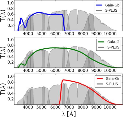
Comparison between the Gaia Gb (blue), G (green), and Gr (red) filters and the S-PLUS filters (light grey).
A2 SDSS and KiDS
Here we present the expected colour terms between SDSS fiters (ugriz) used in SDSS and KiDS and the S-PLUS (ugriz) filters, using two libraries of templates. For stars, we rely on six stellar models from the Pickles library (Pickles 1998). For galaxies, we rely on the bpz templates (Benítez 2000), using a redshift grid z = (0.00, 0.05, 0.20). The different models and the estimated colour terms are shown in Table A1.
Estimated colour terms between the SDSS and the S-PLUS (ugriz) broad-band filters for stars and galaxies. For the former we relied on six stellar models from the Pickles library; for the latter the templates from the bpz code.
| Model | uSDSS–uS-PLUS | gSDSS–gS-PLUS | rSDSS–rS-PLUS | iSDSS–iS-PLUS | zSDSS–zS-PLUS |
|---|---|---|---|---|---|
| Stars | |||||
| o5v | 0.00 | −0.02 | −0.01 | −0.04 | 0.04 |
| b5iii | −0.08 | −0.01 | −0.01 | −0.03 | 0.03 |
| a5v | −0.18 | 0.00 | 0.00 | −0.02 | 0.00 |
| f5v | −0.07 | 0.01 | −0.00 | 0.00 | 0.01 |
| g5v | −0.03 | 0.02 | 0.01 | 0.01 | −0.01 |
| k0v | −0.02 | 0.03 | 0.01 | 0.01 | −0.01 |
| k7v | −0.04 | 0.09 | 0.01 | 0.04 | −0.04 |
| m5v | −0.09 | 0.12 | 0.06 | 0.16 | −0.12 |
| Galaxies | |||||
| Ell (z = 0.00) | −0.01 | 0.04 | 0.02 | 0.03 | −0.07 |
| Sbc (z = 0.00) | −0.07 | 0.02 | 0.02 | 0.04 | −0.06 |
| Scd (z = 0.00) | −0.06 | 0.01 | 0.01 | 0.02 | −0.03 |
| Im (z = 0.00) | −0.05 | −0.01 | 0.01 | 0.02 | −0.04 |
| SB (z = 0.00) | −0.03 | −0.04 | −0.04 | 0.01 | −0.07 |
| Ell (z = 0.05) | −0.05 | 0.02 | 0.02 | 0.03 | −0.07 |
| Sbc (z = 0.05) | −0.06 | 0.02 | 0.01 | 0.04 | −0.06 |
| Scd (z = 0.05) | −0.04 | 0.01 | 0.01 | 0.02 | −0.03 |
| Im (z = 0.05) | −0.04 | −0.00 | 0.01 | 0.02 | −0.04 |
| SB (z = 0.05) | −0.01 | −0.02 | 0.15 | −0.03 | −0.06 |
| Ell (z = 0.20) | −0.14 | 0.11 | 0.03 | 0.04 | −0.05 |
| Sbc (z = 0.20) | −0.05 | 0.05 | 0.02 | 0.03 | −0.06 |
| Scd (z = 0.20) | −0.03 | 0.04 | 0.01 | 0.02 | −0.03 |
| Im (z = 0.20) | −0.01 | 0.02 | −0.01 | 0.02 | −0.04 |
| SB (z = 0.20) | −0.01 | 0.00 | −0.04 | 0.01 | −0.02 |
A3 DES
Similar to what was done in Section A2, we compute the expected colour terms between the DES (griz) and the S-PLUS (griz) broad-band filters. The estimated colour terms are shown in Table A2.
Estimated colour terms between the DES and the S-PLUS (g, r, i, z) broad-band filters. The table includes the colour terms for stars and galaxies. For the former, we relied on six stellar models from the Pickles library; for the latter on templates from the bpz code.
| Model | gDES–gS-PLUS | rDES–rS-PLUS | iDES–iS-PLUS | zDES–zS-PLUS |
|---|---|---|---|---|
| Stars | ||||
| o5v | −0.02 | 0.05 | 0.05 | 0.10 |
| b5iii | −0.01 | 0.03 | 0.03 | 0.06 |
| a5v | −0.00 | 0.02 | 0.02 | 0.00 |
| f5v | 0.01 | −0.01 | −0.00 | 0.01 |
| g5v | 0.02 | −0.02 | −0.01 | −0.03 |
| k0v | 0.03 | −0.03 | −0.01 | −0.03 |
| k7v | 0.06 | −0.07 | −0.05 | −0.08 |
| m5v | 0.06 | −0.17 | −0.13 | −0.25 |
| Galaxies | ||||
| Ell (z = 0.00) | 0.03 | −0.05 | −0.03 | −0.14 |
| Sbc (z = 0.00) | 0.02 | −0.04 | −0.04 | −0.14 |
| Scd (z = 0.00) | 0.02 | −0.03 | −0.02 | −0.06 |
| Im (z = 0.00) | 0.01 | −0.03 | −0.02 | −0.10 |
| SB (z = 0.00) | 0.01 | −0.03 | −0.01 | −0.15 |
| Ell (z = 0.05) | 0.05 | −0.06 | −0.03 | −0.16 |
| Sbc (z = 0.05) | 0.02 | −0.04 | −0.04 | −0.13 |
| Scd (z = 0.05) | 0.02 | −0.03 | −0.02 | −0.06 |
| Im (z = 0.05) | 0.01 | −0.02 | −0.02 | −0.10 |
| SB (z = 0.05) | 0.01 | −0.08 | 0.06 | −0.14 |
| Ell (z = 0.20) | 0.07 | −0.06 | −0.04 | −0.11 |
| Sbc (z = 0.20) | 0.04 | −0.04 | −0.03 | −0.13 |
| Scd (z = 0.20) | 0.04 | −0.03 | −0.02 | −0.07 |
| Im (z = 0.20) | 0.02 | −0.02 | −0.02 | −0.09 |
| SB (z = 0.20) | 0.00 | −0.02 | −0.03 | −0.04 |
A4 From narrow to broad S-PLUS filters
Finally, in this section we provide the internal colour terms for the overlapping narrow-band (J0378, J0515, J0660, and J0861) and the closest broad-band (u, g, r, z) filters in the S-PLUS system. These coefficients are shown in Table A3, using six stellar models from the Pickles library.
Estimated colour terms between the S-PLUS (u, g, r, z) broad-band and narrow-band filters (J0378, J0515, J0660, and J0861). As in previous tables, we relied on six stellar models from the Pickles library.
| Model | J0378–uS-PLUS | J0515–gS-PLUS | J0660–rS-PLUS | J0861–zS-PLUS |
|---|---|---|---|---|
| Stars | ||||
| o5v | 0.06 | 0.20 | 0.13 | 0.00 |
| b5iii | −0.23 | 0.10 | 0.11 | 0.00 |
| a5v | −0.54 | −0.03 | 0.11 | −0.00 |
| f5v | −0.31 | −0.12 | −0.00 | 0.00 |
| g5v | −0.26 | −0.17 | −0.05 | 0.01 |
| k0v | −0.24 | −0.17 | −0.09 | 0.02 |
| k7v | −0.27 | −0.11 | −0.26 | 0.00 |
| m5v | −0.26 | −0.33 | −0.52 | 0.03 |
