


ABSTRACT
Stellar feedback plays a significant role in modulating star formation, redistributing metals, and shaping the baryonic and dark structure of galaxies – however, the efficiency of its energy deposition to the interstellar medium is challenging to constrain observationally. Here we leverage HST and ALMA imaging of a molecular gas and dust shell (|$M_{\mathrm{ H}_2} \sim 2\times 10^{5}\, {\rm M}_{\odot }$|) in an outflow from the nuclear star-forming ring of the galaxy NGC 3351, to serve as a boundary condition for a dynamical and energetic analysis of the outflowing ionized gas seen in our MUSE TIMER survey. We use starburst99 models and prescriptions for feedback from simulations to demonstrate that the observed star formation energetics can reproduce the ionized and molecular gas dynamics – provided a dominant component of the momentum injection comes from direct photon pressure from young stars, on top of supernovae, photoionization heating, and stellar winds. The mechanical energy budget from these sources is comparable to low luminosity active galactic neuclei, suggesting that stellar feedback can be a relevant driver of bulk gas motions in galaxy centres – although here ≲10−3 of the ionized gas mass is escaping the galaxy. We test several scenarios for the survival/formation of the cold gas in the outflow, including in situ condensation and cooling. Interestingly, the geometry of the molecular gas shell, observed magnetic field strengths and emission line diagnostics are consistent with a scenario where magnetic field lines aided survival of the dusty ISM as it was initially launched (with mass-loading factor ≲1) from the ring by stellar feedback. This system’s unique feedback-driven morphology can hopefully serve as a useful litmus test for feedback prescriptions in magnetohydrodynamical galaxy simulations.
1 INTRODUCTION
Feedback from young stars throughout their lifetime and at their death is thought to be a significant contributor to the energy budget of the interstellar medium (ISM) within star-forming galaxies. Stellar evolution theory has provided many quantitative predictions for how feedback [stellar winds, ionizing radiation, metals, and supernovae (SNe)] vary as a function of time, metallicity, and initial stellar mass function (IMF) within a population of stars (c.f. Leitherer et al. 1999). However, the subsequent impact of these events on the host galaxy has been characterized best through numerical hydrodynamic simulations of galaxies.
The inclusion of baryonic physics within galaxy simulations has helped solve a plethora of discrepancies between dark matter (DM) only simulations and observed galaxy properties (Katz 1992; Navarro & White 1993). Newer implementations of feedback (e.g. Stinson et al. 2006; Hopkins et al. 2014) proved to be a crucial ingredient in removing low angular momentum gas within galaxies – helping simulations form realistic low bulge fractions and radially extended thin galactic discs (Governato et al. 2004). In addition, SNe feedback has been shown to drive metals into the circumgalactic media via outflows (e.g. Shen et al. 2013; Turner et al. 2016), which are observed commonly around galaxies of many types and masses (e.g. Werk et al. 2016) – and this process is also thought to modify the cuspy DM profiles in low-mass galaxies (Di Cintio et al. 2014).
The ever improving numerical resolution among hydrodynamical simulations has opened up a wealth of new investigative possibilities, but also added complexity in how sub-grid feedback prescriptions are modelled. Such prescriptions may try to address for example: the efficiency of photon pressure on dust (Hopkins, Quataert & Murray 2011), thermalization of the energy dumped into the ISM by feedback, or porosity/escape fraction effects (Krumholz & Thompson 2013). Recent studies have also focused on the role played by ionizing radiation from young massive stars – as the energy budget could be comparable to the SNe of a given simple stellar population in some cases (e.g. Rosdahl et al. 2015).
Reproduction of observed galaxy mass functions, and even small-scale dynamical, chemical, and structural features (Few et al. 2012; Renaud et al. 2013; Schroyen et al. 2013; Martig, Minchev & Flynn 2014; Dutton et al. 2016; El-Badry et al. 2016; Read et al. 2016; Di Cintio et al. 2017) is a great success for these simulations and models. However, concerns about the degenerate behaviour of many of the complex prescriptions used for feedback or star formation (e.g. Cloet-Osselaer et al. 2012) provides ample motivation for the observational community to continue to provide useful constraints for calibration of these methods.
Direct observations of large-scale outflows offer a natural window into the energetics provided by feedback sources (e.g. Martin 2005; Lopez et al. 2011). Finding a boundary condition for the initial time or total distance of the outflow event is often observationally problematic to establish, and prevents a complete evolutionary picture and energetic accounting of galactic systems. Nevertheless instantaneous observational quantities such as the outflow mass-loading factor (|$\eta = \dot{M}_{\rm out} / \mathrm{ SFR}$|) are essential to calibrate energy and momentum deposition in simulations (Davé, Finlator & Oppenheimer 2011; Schroetter et al. 2016). Additionally several indirect tests of the impact of feedback processes have been performed at high redshift, and in the local Universe, such as exploring the radial metallicity profiles of disc galaxies, which were shown to be sensitive to the feedback prescriptions used in simulations (e.g. Pilkington et al. 2012; Gibson et al. 2013; Schroyen et al. 2013; El-Badry et al. 2016; Starkenburg et al. 2017).
Motivated by the ambitions of modern galaxy simulations and past observational tests, in this paper we explore stellar feedback at intermediate scales, where the observational resolution is comparable to that of current galaxy simulations. We present kinematic observations of the multiphase ISM in the nuclear ring galaxy NGC 3351, as part of our VLT/MUSE TIMER survey (PI: Gadotti),1 with the goal of understanding the survival of cold gas in outflows and providing quantitative tests for sub-grid stellar feedback prescriptions.
NGC 3351 is comparable to our own Galaxy in total stellar mass, metallicity (|$M_{*} = 3.1\times 10^{10}\, {\rm M}_{\odot }$|, Z/Z⊙ = 0.4) and star formation (SFR|$= 0.6\, {\rm M}_{\odot }\, {\rm yr}^{-1}$| in the nuclear ring alone; Gadotti et al. 2019). As with all of the galaxies in the TIMER survey, it was selected because of its strongly barred morphology and presence of a nuclear ring – with its classification listed as |$(R^{^{\prime }})SB(r,bl,nr)a$| in Buta et al. (2015). NGC 3351 exhibits dust lanes throughout the spiral arms, along the bar and nuclear ring – along with a transverse dust lane offset from the nuclear ring and orthogonal to the bar lanes. This feature will be discussed throughout this work and is indicated by the arrow in Fig. 1. NGC 3351 is considered an isolated field galaxy (Young et al. 1996) and NED lists the closest neighbour (Messier 96) as having projected distance and redshift separations of Dsep = 125 kpc and Δcz = 120 km s−1, respectively (https://ned.ipac.caltech.edu/forms/denv.html) – implying minimum interaction time-scales of at least 1000 times longer than the dynamical time of the nuclear ring in NGC 3351. While this is a heterogeneous source catalogue of detections, the list appears luminosity complete down to values of L ∼ 4 × 10⁵ L⊙. Notably, NGC 3351 has no evidence for an AGN (from emission line diagnostics; e.g. Gadotti et al. 2019) and as such is often used as a control galaxy in studies on AGN properties and their feeding mechanisms (e.g. Colina et al. 1997).
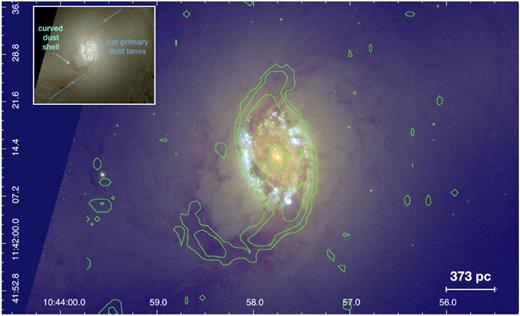
HST WFC3 colour composite image of the central region of NGC 3351 made as part of the LEGUS survey (https://legus.stsci.edu/) from F814W, F555W, and F336W exposures. In the inset, we show a zoomed-out image of the galaxy, where we can see the ‘primary dust lanes’ caused by bar-driven shocks (their length and orientation are indicated with the blue lines); the elliptical dust shell (which is pointed to by the arrow) is evident as a curved transverse feature, orthogonal to the ‘primary’ feeding lanes of the bar. This primary shell is coincident with molecular gas emission in the ALMA moment 0 CO map (green contours).
The MUSE observations presented here show a serendipitous and visually clear signature of a planar/radial outflow from the nuclear ring of NGC 3351 in the ionized gas flux and kinematic maps. This was accompanied by identification of a unique concentric shell of dust and molecular gas in archival HST and ALMA observations. The location of this transverse dusty gas shell is unexpected from a purely gravitational standpoint (see Section 3), which teases at a common evolution with the ionized gas, likely due to feedback from the star-forming nuclear ring. In addition, as seen and discussed in other galactic outflows, the presence of cold molecular gas may be naively unexpected given the hot, energetic phenomena that provide kinematic feedback in the ISM (c.f. McCourt et al. 2018). This system offers a relatively complete observational framework to test many of the theoretical models proposed for cold gas formation and survival in outflows.
1.1 A stellar feedback scenario for the ISM in NGC 3351
The clear signatures of warm gaseous outflow in our data, together with the archival ALMA and HST data of the cold gas and dust, hint at a scenario for the transverse dust-lane feature: (1) stellar feedback from the nuclear ring pushes out the cold gas shell, which was initially co-located with the nuclear SF ring, thus forming a low-density cavity. (2) Warm ionized gaseous outflows, which fill the cavity, shock with the underlying multiphase ISM. (3) The survival of the cold phase during the outflow could have been aided by magnetic fields initially permeating through the dusty ISM, which is consistent with a vertically constrained outflow for the hot ionized gas.
While in principle other scenarios such as cold gas inflows or fly-by with a satellite galaxy, could potentially be responsible for the origin of the curved dust lane observed in NGC 3351, we discuss in Section 3.3 why these are less likely than the feedback scenario proposed here – and note the isolation criteria mentioned above rule out a fly-by origin for the feature given the relevant time-scales. In what follows, we quantitatively evaluate the validity of this feedback scenario and scenarios for the survival of the cold gas, in the context of the data, stellar feedback models, and numerical simulations. The observations are presented in Section 2 of this paper. In Section 3 we present hydrodynamical simulations tailored to reproduce the effect of the gravitational potential of NGC 3351 on the gas dynamics. We analyse the emission-line and dynamical properties of the ionized and molecular gas in Section 4. We present a model for the feedback processes and dynamics of the outflow observed in this system in Section 5, and discuss the survival of molecular gas in outflows in Section 6. Implications of our findings for feedback parametrizations in simulations and further astrophysical questions are discussed in Section 7. We summarize this study with our main conclusions in Section 8. Where necessary we adopt a Hubble constant of H0 = 67.8 km s−1 Mpc−1 and Ωm = 0.308 with a flat topology (Planck Collaboration et al. 2016).
2 OBSERVATIONS AND ANALYSIS
As much of the analysis in this work surrounds the dynamics, stellar populations, and gas content of the inner region of NGC 3351, we briefly describe some of the relevant features and their properties for context. Fig. 1 highlights several of the structures of interest in our study. The nuclear ring is evident in molecular gas and exhibits ongoing star formation typical of these structures. In NGC 3351, the nuclear ring has a radius of ∼250 pc and width of ∼50−100 pc. The bar of the galaxy, which can be traced in the image through the linear dust feeding lanes, is orientated 112° from North (Salo et al. 2015), and has a semimajor axis of 2.7 kpc (Kim et al. 2014). Given the derived bar mass fraction from photometric decompositions (Kim et al. 2014) and the total stellar mass of NGC 3351 (Gadotti et al. 2019), the bar stellar mass is approximately 2.8 × 10⁹ M⊙. Part way along the bar (D ∼ 1 kpc) there is a well-defined transverse shell of dust and molecular gas which is orthogonal to the bar feeding lanes, and concentric to the nuclear ring. This feature has an arc length of approximately 1 kpc and in contrast to the bar, the molecular gas observations (see Section 2.2 below) suggest a gas mass of ∼6 ± 4 × 10⁵ M⊙ for the shell. We now highlight below the observations and data analysis steps which we will use to analyse the genesis of this feature and shed light on the evolutionary mechanisms at play in the inner regions of barred galaxies.
2.1 MUSE spectroscopy
Details on the observations, data reduction, and analyses of the TIMER MUSE data can be found in Gadotti et al. (2019); here we provide a summary of the most relevant aspects. The observations with MUSE were performed during ESO Period 97, using the normal instrument set-up, which yields a spectral resolution of 2.65 Å and a spectral coverage from 4750 to 9350 Å. The image quality during the observations of NGC 3351 was ∼0.6 arcsec. We targeted the central 1 × 1 arcmin2 of the galaxy and used dedicated empty sky exposures to remove the contribution from the background.
We used the MUSE pipeline v1.6 (Weilbacher et al. 2012) and employed the standard calibration plan to reduce the data. In the first step of the data reduction, each science frame is calibrated separately to take out instrumental effects (bias, flat-field, and illumination correction). The spectra are then extracted and calibrated in the wavelength direction using the standard line spread function mapping. The calibrated science frames are combined into the final data cube after performing flux calibration, background subtraction, astrometric registration, correction for differential atmospheric refraction, and resampling of the data cube based on the drizzle algorithm. For some of the science frames, we used a background frame created from interpolating background frames taken before and after the science exposure. This is done to account for variations in the background and best reproduce the background at the time of the science exposure. In the last step of our data reduction process, after employing the MUSE pipeline, we have also implemented a method to improve the removal of residual background emission from the data cube using principal component analysis.
To obtain information from the emission lines in the MUSE cube, such as flux and kinematics (to derive velocity and velocity dispersion), we used PyParadise, which is an extended python version of Paradise, described in Walcher et al. (2015) We first derived the contribution of stars to the spectra by using Voronoi binning to increase the signal-to-noise ratio to a target of S/N = 40, and then fitted the resulting spectra with a combination of template stellar spectra taken from the Indo-US spectral library (Valdes et al. 2004), interpolating over emission lines and residual sky lines. PyParadise also fits the stellar kinematic parameters, and the resulting best-fitting spectra are subtracted from the observed spectra spaxel by spaxel. We then fitted all major emission lines, spaxel by spaxel, with Gaussian functions coupled in line width and radial velocity. By forcing the kinematics to match we ensure that line ratios are computed for physically connected regions. To estimate the errors on all measured parameters 100 Monte Carlo realizations were run, where in each trial noise returned from the MUSE pipeline was used to inject random noise in the spectra prior to the aforementioned analysis steps.
2.2 ALMA and HERACLES molecular gas observations
To complement our MUSE observations, we used archival data of molecular gas emission in NGC 3351. In order to obtain gas masses and global kinematic parameters, we used the public CO(2–1) maps from HERACLES2 (Leroy et al. 2009). These observations were taken with the IRAM 30m telescope, and recover all the flux at an angular resolution of 13 arcsec (640 pc at the assumed distance of 10.1 Mpc; Moustakas et al. 2004). Given the near-solar metallicity of the galaxy [12 + log(O/H) = 8.9; Moustakas et al. 2010], we use the standard Milky Way conversion factor |$\alpha _\mathrm{CO} = 4.4\, \rm M_\odot$| (K km s−1 pc2)−1 and assume a fixed line ratio CO(2–1)/CO(1–0) = 0.8 (Leroy et al. 2009).
To pinpoint the detailed distribution and kinematics of molecular gas in the vicinity of the nuclear ring, we utilized archival ALMA Early Science Cycle 2 observations from project 2013.1.00885.S (PI: Karin Sandstrom). We downloaded the calibrated and imaged datasets from the ALMA archive,3 corrected for the response of the primary beam, and extracted the channels corresponding to the line 12CO(1–0), with a rest-frame frequency of 115.27 GHz. These ALMA Band 3 observations reach a typical rms sensitivity of ∼6 mK per 1.92 MHz-wide channel (a velocity resolution of 5 km s−1), which results in a S/N ∼ 20−40 in the star-forming ring, and S/N ∼ 5−10 in the transverse shell. The synthesized beam is 2.0 × 1.2 arcsec (100 × 60 pc; PA = 27°).
We converted the ALMA cube to brightness temperature and constructed moment maps for the 12CO(1–0) line: moment 0 corresponds to the integrated intensity, moment 1 is the intensity-weighted velocity field, and moment 2 represents the intensity-weighted velocity dispersion. We integrated emission for channels in the window 114.902–115.031 GHz, using line-free channels to estimate the noise (remaining channels in the frequency range 114.878–115.068 GHz). We use a sigma-clipping method for moments 0 and 1, to avoid being biased by noise; our preferred maps use a threshold of 4σ, where σ is the rms noise in line-free channels and is calculated on a pixel-by-pixel basis. This means that, for each spatial pixel, we mask any spectral channels with values below four times the rms obtained for that specific position; this is equivalent to running the task immoments4 within casa (McMullin et al. 2007) with the parameter includepix set to a minimum value of 4 rms, where rms is the 2D map corresponding to the standard deviation on line-free channels. It is important to impose a threshold that depends on the position in the map, as noise increases towards outer regions as a result of the primary-beam correction.
We have experimented with different thresholds and different integration windows, confirming that the maps are sufficiently robust for our purposes in the areas of interest. For the moment 2 map we use the ‘window method’ (Bosma 1981), which captures more low-level emission, providing a better estimate of the real velocity dispersion. We first impose a 4σ threshold to identify pixels with significant emission, but then consider all emission in those significant pixels, only limited by a window in frequency. We ignore any spatial pixels below a threshold of 4σ. We consider the remaining spatial pixels as significant, and define a range of channels (the frequency window) where emission is considered to compute the second-order moment value. This window is iteratively expanded (started from the channel of peak emission) until the average continuum emission outside the window converges according to the criterion from Bosma (1981). The maps agree well with 13CO(1–0) observations from the ALMA Early Science Cycle 2 project 2013.1.00634.S (PI: Adam Leroy).
2.3 Ancillary imaging data
Archival HST WFC3 images (Program ID 13364; PI Calzetti) in the F336W and F814W filters were obtained from the MAST archive. The original observations were taken on 2015 April 23 and subsequently processed with AstroDrizzle. The F814W and F336W images have exposure times of 908 and 1062 s, respectively. A three-colour HST composite image from the LEGUS survey (Calzetti et al. 2015) is shown in Fig. 1, with the ALMA CO moment 0 map overlaid.
2.4 Kinematic analysis
To constrain the large-scale CO rotation curve we ran the task ROTCUR within GIPSY (van der Hulst et al. 1992) on the moment-1 map obtained with HERACLES, which has a much larger field of view than the ALMA observations. Given the relatively low spatial resolution of HERACLES, we assume that the moment-1 map predominantly traces circular rotation and is not too affected by streaming motions. We performed an independent check of the rotation curve by assuming different sets of input parameters for the systemic velocity (Vsys), inclination (i), position angle (PA), and the coordinates of the centre (x0, y0). We allowed Vsys to vary from 760 to 790 km s−1 in steps of 2 km s−1. The PA was allowed to vary from 185 to 195 in steps of 1°, and a range of 30−60 degrees was explored for the inclination, in steps of 5 degrees. We initially fixed the kinematic centre visually (x0 = 110, y0 = 110, corresponding to RA = 10:43:57.793, Dec. = +11:42:14.20) but we also confirmed that shifting the centre by 2 pixels or more (corresponding to 4 arcsec) in any directions leads to clearly poorer residuals – specifically when inspecting the residuals of the model velocity field and the observed line-of-sight velocity maps [(Vmod − VLOS)2]. We deprojected, derived the corresponding V(R), and compared the final residuals by eye. Both ROTCUR and these tests suggest that the PA is well constrained by PA ∼ (192 ± 2)°, Vsys ∼ (776 ± 4) km s−1, and the rotation curve is relatively insensitive to inclination changes (i ∼ 40−50°). This agrees with estimates from Buta (1988), Tamburro et al. (2008), and Mazzalay et al. (2014) using a variety of tracers.
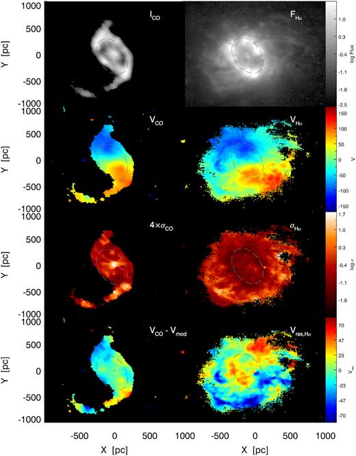
Left column: Molecular gas from top to bottom are the molecular gas intensity (in K km s−1), rotation velocity, velocity dispersion, and molecular gas residual velocity (VCO − Vcirc). Right panel: Ionized gas H α flux (in erg s−1), velocity (in km s−1), velocity dispersion, and ionized gas residual velocity (VHα − Vcirc; see equation 1). An ellipse is reproduced in each panel for reference. Symmetric radial outflows up to ∼70 km s−1 are clearly evident in the bottom right panel.
To further understand whether the high-velocity dispersion of H α is dominated by turbulent or gravitational sources, we leverage our multiple kinematic tracers to perform a decomposition of the H α velocity dispersion (c.f. Weijmans et al. 2008). The purely gravitational component of the velocity dispersion can be extracted by comparing the H α rotation velocity to the true circular velocity (as traced by the CO gas or derived from stellar dynamical models). In the latter case we have derived the circular velocity from the stellar kinematics using Jeans Axisymmetric Models (JAM; Cappellari 2008). The stellar dynamical model for NGC 3351 was constructed identical to the descriptions in Leung et al. (2018), and we refer readers to that study for a detailed description. As shown in Leung et al. (2018), the circular velocities derived from JAM agree well with that derived using CO. This is also the case here, as seen in Fig. 6 where the red circular velocity curve derived using JAM is in good agreement with the green circular velocity curve derived from CO.
3 HYDRODYNAMICAL MODELLING OF THE GAS
As discussed above, and as shown in a number of observational and theoretical studies (e.g. Jorsater, Lindblad & Boksenberg 1984; Teuben, Sanders, Atherton & van Albada 1986; Sandage et al. 1988; Athanassoula 1992; Piner, Stone & Teuben 1995; Kim et al. 2012; Sormani, Binney & Magorrian 2015) in barred galaxies gas accumulates along two well defined ‘primary dust lanes’ (see Fig. 1) which run along the leading edges of the bar, funnelling gas to the nuclear region. These form due to shocks induced by the rotating non-axisymmetric gravitational potential, and the morphology of the dust lanes therefore depends on the strength of the non-axisymmetric component of the potential, as well as on the angular frequency at which the bar rotates (Athanassoula 1992).
To model the gas dynamics due purely to the underlying gravitational potential of NGC 3351, we run a suite of hydrodynamic simulations, which explicitly use the observed mass distribution of the galaxy. While the ‘primary’ dust lanes observed in the galaxy are very likely due to the gas-dynamical response to the gravitational potential, we want to explore whether the curved dust lane is also due to the gravitational potential, or whether some other processes (such as for example stellar feedback) are necessary to create it.
3.1 Gravitational potential
The method we use for calculating the potential due to the stellar component involves a straightforward three-dimensional integration over the density distribution of the target galaxy, which is described in detail in Fragkoudi et al. (2015). We first obtain a stellar mass map for the galaxy from the 3.6 μm NIR image, which is cleaned from foreground stars and is deprojected to be face-on (Querejeta et al. 2015). To obtain the stellar mass surface density we assign a mass-to-light ratio of M/L = 0.6 (Meidt et al. 2014; Erroz-Ferrer et al. 2016; Röck et al. 2016; Fragkoudi, Athanassoula & Bosma 2017) to each pixel in the NIR image, which has been shown to be suitable for a wide range of ages and metallicities of the underlying stellar populations (Meidt et al. 2014). We then assign a height function in order to account for the thickness of the disc (assuming a relation between the scale height and scale length of the galaxy according to Kregel, van der Kruit & de Grijs 2002), and integrate over the density distribution to obtain the gravitational potential of the disc. We add a dark matter halo with parameters such that the outer parts of the model rotation curve match the observed rotation curve of the galaxy (see Fig. 6 and Section 2.4). Therefore the rotation curve derived for NGC 3351 (in Section 2.4) is used as a constraint in building our gas dynamical models. As has been shown to be the case for massive disc galaxies (e.g. Kranz, Slyz & Rix 2003; Courteau & Dutton 2015; Fragkoudi, Athanassoula & Bosma 2017) the galaxy is baryon dominated in the central regions, and thus the dark matter potential contributes little to the total gravitational potential in the regions we are interested in (i.e. within 2 kpc). This set-up allows us to initialize a simulation which is tailored to the observed mass distribution of NGC 3351, thus enabling us to study the dynamics of gas in this galaxy.
3.2 Gas response simulations
The gas response simulations are produced with the hydrodynamic adaptive mesh refinement (AMR) grid code ramses (Teyssier 2002). The simulations are run in two dimensions, since, to zeroth order, gas is confined to a thin plane in disc galaxies. The set-up used for these gas-dynamical simulations is described in Fragkoudi et al. (2017).
The initial conditions of the simulations consist of a two-dimensional axisymmetric gaseous disc, with a homogeneous density distribution in hydrostatic equilibrium. The disc is truncated using an exponential tapering function.5 The gas is modelled to be isothermal, with adiabatic index 5/3 – corresponding to H i gas (neutral atomic hydrogen) and is assigned a sound speed of 10 km s−1, corresponding to characteristic temperatures of the ISM.
In order to avoid transient features in the disc, we introduce the non-axisymmetric potential gradually over a finite period of time, – specifically ∼3 bar rotations, in accordance with previous studies which calibrated this empirically (Athanassoula 1992; Patsis & Athanassoula 2000). After the non-axisymmetric potential has been fully introduced, the gas settles in a stable state and we use subsequent snapshots to examine the shocks and gas morphology which are produced purely due to the gravitational potential of the system.
We run a suite of simulations in this set-up with different values of the bar pattern speed, to find the best-fitting model, defined as the model which best reproduces the gas morphology of NGC 3351 in the bar region (i.e. which has primary bar dust lanes in the correct locations6). We first scan the parameter space by running five simulations with |$\mathcal {R}$| in the range from 1 to 2 (which is the range of values expected from theory and observations; e.g. Athanassoula 1992; Corsini 2011), where |$\mathcal {R}= R_{\rm CR}/R_{\rm bar}$|, RCR is the corotation radius and Rbar is the bar length. Bars are considered slowly rotating if |$\mathcal {R}\gt 1.4$| and fast rotating if |$\mathcal {R}\lt 1.4$| (see Debattista & Sellwood 2000). We found that a fast bar, i.e. with |$\mathcal {R}\lt 1.4$| (which corresponds to values of the bar pattern speed between ∼33 and 38 km s−1 kpc−1) gives a better fit to the gas morphology. We then explore this region of the parameter space, by running five simulations with pattern speeds varying by 1 km s−1 kpc−1, to identify more precisely the best-fitting bar pattern speed. Finally, the best-fitting model has |$\mathcal {R}\sim$|1.15 – which corresponds to a bar pattern speed of ∼35 km s−1 kpc−1. We emphasize that none of the models we explored in this analysis contain a secondary curved dust lane, i.e. even models with much slower or faster bars did not contain such a feature.
3.3 Origin of the transverse dust shell
In Fig. 3 we show the surface density of the gas in the fiducial simulation (top panel), the gas velocity field vlos (middle panel), and the residual velocity vres = vlos – vcirc (bottom panel). In all panels we rotate the model to have the same projection in the plane of the sky as NGC 3351.
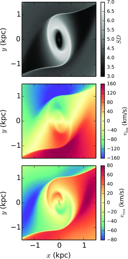
Gas surface density for the best-fitting simulation (in arbitrary units of surface density). There is only one pair of shocks formed at the leading edges of the bar which will produce the linear feeding dust lanes seen in the galaxy – however there is a clear absence of any analogous transverse dust shells in this purely gravitational simulation.
By examining the morphology of the gas in the simulation (top panel) we see that gas accumulates mainly in the nuclear ring of the galaxy and along the two ‘primary dust lanes’ which are located on the leading edge of the bar. Gas accumulates in shocks along the leading edges of the bar (where dust lanes are formed) due to the torques induced by the underlying non-axisymmetric potential. However, we do not find in any of our models evidence for a secondary curved dust lane. By examining the second panel of Fig. 3, we see that the overall velocity field of the gas matches quite well the observed velocity field of the CO gas in NGC 3351 (see Fig. 2).
The fact that the transverse dust lane of NGC 3351 is not produced in the hydrodynamic simulations suggests that it is not of a dynamical origin, i.e. it is not caused by the underlying non-axisymmetric potential (as is the case for the primary dust lanes seen on the leading edges of the bar in NGC 3351). This statement is given special weight in the case of our AMR simulations as they directly use the derived potential of NGC 3351. Therefore, additional processes likely related to stellar feedback, which are not captured in the simulations, are necessary to reproduce the observed shocks and gas features.
As suggested in Section 1.1 and discussed in more detail in the next sections, the cold gas currently seen in the transverse dust lane was likely pushed there from the nuclear ring region, by stellar feedback processes. While it is possible that other mechanisms, such as tidal interactions, inflows or the ‘wiggle’ instability, might be responsible for the creation of the curve dust lane, we find these less likely than the scenario we propose, due to the reasons given below.
As noted in Section 1, NGC 3351 is a relatively isolated galaxy, with its closest neighbour having a projected distance of ∼125 kpc; it is therefore unlikely that the curved dust lane is triggered by a tidal interaction due to a close companion. On the other hand, if there were in-plane inflow through the disc causing this feature, this should be captured by our gas-dynamical model (which models the gas dynamics in the disc due to the gravitational potential). On the other hand, extra-planar flows, such as those caused by fountain flows, can be outwards or inwards moving, however the inwards motion is expected to be small, of the order of approximately a hundred parsecs (see e.g. Fraternali & Binney 2008). Therefore extra-planar gas ejected from star forming regions – such as the spiral arms – is unlikely to reach the small radii which we consider here through a fountain flow (see e.g. Fraternali & Binney 2008; Pezzulli et al. 2015; DeFelippis et al. 2017). Furthermore, as discussed below in Section 4.2, the residual CO velocities are inconsistent with the CO gas in the transverse dust lane moving inwards. Other effects related to gas instabilities in nuclear rings, such as for example the ‘wiggle’ instabilities described in Sormani et al. (2017), are also unlikely to produce such large-scale features like the curved dust lane. We therefore conclude that the most likely scenario is one in which feedback from the nuclear ring is responsible for creating the curved dust lane.
Fig. 1 shows that, at present day, the cold molecular CO gas and the dust (as traced in optical colours) are co-located at the position of the transverse shell. This strongly suggests that the initial driving mechanism to move this feature from the nuclear ring outwards, moved the dust and molecular gas together. In addition the CO gas and dust appear to be evacuated in the area closest to the nuclear ring, suggesting some dynamical movement of these cold dense gas tracers.
Fig. 4 shows that the subsequent radial expansion of the warm ionized gas has filled the cavity bounded by the outer transverse dust shell. This low-density ionized medium appears nearly completely contained by the extent of the CO/dust shell, as is also suggested by studies which found X-ray emission contained within this cavity (Swartz et al. 2006).

H α flux (left), velocity dispersion (middle), and residual velocity (right) fields of NGC 3351 are shown in colour scale. Overlaid as contours is the ALMA CO(1–0) moment 0 map, which clearly encloses the ionized outflows to the south-west of the nuclear ring.
4 PROPERTIES OF THE IONIZED AND MOLECULAR GAS
Here we seek to use the observations of the molecular and ionized gas kinematics and densities, to understand the dynamical state of the outflow in NGC 3351. Quantifying the mechanical energy, outflowing velocities, and morphological structure of the outflow will allow us to make more rigorous tests for the origin of the outflow in our analytic and numerical models.
From the residual velocity map in Figs 2 and 4 we can see a strong bisymmetric radial flow of the ionized gas up to ∼70 km s−1. As indicated by the ellipses in Fig. 2 (which mark the location of the nuclear ring), this radial flow covers the area from the nuclear SF ring (where the H α peak flux is) and passes through a region of high-velocity dispersion near the inner edge of the transverse CO shell.
4.1 Emission line diagnostics
The bulk of the underlying ionized gas velocity field in Fig. 2 has a rotation axis orthogonal to this radial outflow. Along the bar (roughly parallel to the minor axis of the ring), the LOS velocity field is close to zero – which suggests that shocks should occur in the cavity where the outflowing gas collides with this stationary (or even partly orthogonally rotating) ISM.
We compute the star formation rate following the Kennicutt (1998) relation (|$\mathrm{ SFR} = L_{\mathrm{ H}\,\alpha }\,1.26\times 10^{41}\, {\rm erg \,s}^{-1}$|), after correcting the H α emission for extinction using the prescriptions in Calzetti et al. (2000) and estimating the E(B − V) from the Balmer decrement. The electron densities were computed using the extinction corrected fluxes of the [S ii] doublet emission lines (at λ = 6716, 6731 Å) following equation 1 and table 1 of Kaasinen et al. (2017).
Relevant gas time-scales at the outflow front.
| Time-scale | Value | Notes |
|---|---|---|
| Outflow travel | Section 3.2, Appendix B | |
| log texp | |$7.2_{-0.6}^{+0.6}$| | |
| Turbulent dissipation | Equation (7) | |
| log tdiss | |$6.9_{-0.1}^{+0.2}$| | |
| Crushing | McCourt et al. (2018) | |
| log tcrush | |$6.3_{-0.6}^{+0.4}$| | |
| Entrainment | McCourt et al. (2015) | |
| log tentr | |$6.9_{-1.0}^{+0.7}$| | |
| Cooling | Equation (8) | |
| log tcool | |$7.9_{-0.8}^{+2.0}$| | for η = 0.85 ± 0.6 |
| Advection | Equation (9) | |
| log tadv | |$5.8_{-0.4}^{+0.2}$| | For η = 0.85 ± 0.6 |
| Conduction | Thompson & Krumholz (2016) | |
| log tcond | 6.4 | Excluding magnetic fields |
In Fig. 5 we show the spaxels in the MUSE field, and their position on the BPT emission line diagnostic diagram (c.f. Baldwin, Phillips & Terlevich 1981). The spaxels outside the nuclear SF ring fall clearly in the shocked region of the BPT diagram (e.g. Kewley et al. 2001; Kauffmann et al. 2003).
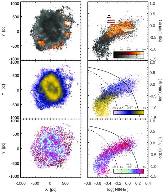
Spatial maps (left) and BPT diagram (right) of the central star forming ring and surrounding area of NGC 3351. The top panel shows the pixels greyscale coded by σH α, with a subset of high dispersion (σ ≥ 125 km s−1) pixels shown in the orange colour bar and outlined in black. These spaxels have emission line ratios consistent with fast shock models of the observed velocity (coloured tracks on the same velocity scale, spanning from left to right magnetic field strengths from 1 to 100 μG). Middle panel shows the SFR surface density, while bottom panel shows electron density, indicating that the high electron densities in the outer region are due to compressive shocks rather than high SFRs. Solid (dashed) black lines show the upper (lower) theoretical limits expected for SF (AGN) galaxies, respectively (e.g. Kewley et al. 2001; Kauffmann et al. 2003).
As a strong consistency check, we can ask if the emission line ratios we observe are consistent with coming from gas with shock velocities close to the ionized gas velocity dispersion we measure.
In the top panel of Fig. 5 we show the result of fast-shock models using the MAPPINGS-III code (Allen et al. 2008), which predict the emission line ratios for shocked gas of a given density moving at a particular velocity, in a given magnetic field. The spaxel values for the MUSE emission line ratios are shown in that figure, and the subset of pixels in the high velocity dispersion region of the cavity are colour coded by their velocity dispersion. The shock models (here run for solar metallicity and densities of |$n_{\mathrm{ e}} = 100\, {\rm cm}^{-3}$|) of different magnetic field strengths (notches along the tracks from 1 to 100 μG) are also colour coded by velocity and show good agreement with respect to the observed velocity and emission line ratios in the cavity.
The BPT diagram emission line diagnostics and shock models indicate that a significant amount of ionizing radiation did not precede expansion of the dusty molecular shell and alter the emission line ratios in the region outside the nuclear ring (e.g. the line ratios are inconsistent with a precursor ionization front). Precursor shock models for our densities and magnetic fields predict |${\rm log}({\rm O}\,\small {III}/\mathrm{ H}\,\beta)$| ratios greater than zero, which are above our measured values (Fig. 5). This provides important indirect evidence that the bulk of the ionizing radiation in the initial starburst was absorbed by the dusty gas shell and transferred momentum into this structure through direct photon pressure.
The middle panel of Fig. 5 shows that the emission line ratios for the region outside the SF ring are indeed in the classical region associated with shocks (c.f. Kewley et al. 2001). The bottom panels show indications that the cavity contains a few spaxels with electron densities sometimes approaching that of the ring (log ne ∼ 4). However there is clear stochasticity in the on-sky map which led us to check with both a binned analysis of the MUSE cube and a locally weighted regression smoothing (Cappellari et al. 2013) whether these values were representative of the average electron density in the cavity. In addition we tested whether temperature corrections (using the local velocity dispersion σH α and mean molecular weight μ to compute a post-shock temperature [Ts = 1.1μ(σH α/1000)2 keV] to the electron density would alter the electron density map. All three checks suggested that the electron density between the shell and the ring is higher in regions of large velocity dispersion (even in the ne maps where shock temperature was not used to correct the electron density), and that the typical cavity electron density is closer to 2.0 ≲ log ne ≲ 3.0. The stochasticity is likely due to the weak nature of the sulfur lines used to derive the density and our spectral resolution – despite imposing cuts on the relative flux error for H α (≤0.05) and the [S ii] lines themselves (≤0.5). To summarize, the average, error on the mean, and standard deviation of the spaxel electron densities in regions of the ring (defined as where the SFR surface density exceeds logΣSFR = 0.5), the cavity (the high dispersion pixels outlined in red in between the shell and ring in the upper left panel) and the remainder of the area outside of the ring were found to be: logne,Ring = 3.07 ± 0.01 (σ = 0.16), logne,Cavity = 3.05 ± 0.04(σ = 0.61) and logne,outside = 2.77 ± 0.04 (σ = 0.60). While there is clear uncertainty and difficulty in statistically differentiating the electron densities between the regions – these tests and the spatial correspondence of enhanced electron densities and regions of high-velocity dispersion, hint that the values of ne in the cavity region are not due to high SFR surface densities – instead they may be intrinsic to, and enhanced by, the compressive gas motions which generated the shocks. This is indirectly given support by the shock models in the top panel, which reproduce the observed line diagnostics when using cavity densities of ne = 100, and is also consistent with the presence of X-ray emission in this region (Swartz et al. 2006).
4.2 Gas dynamics
The emission line diagnostics suggest a turbulent origin for the large H α velocity dispersion in the cavity. As an additional check, in Fig. 6 we show a decomposition of the Hα velocity dispersion into gravitational and non-gravitational (turbulent) components. As described in Section 2.4, this is possible by comparing the H α rotation curve to the ‘true’ circular velocity – as traced independently by the dynamically cold CO rotation curve (and confirmed by dynamical modelling of the stellar kinematics; e.g. Leung et al. 2018). The ionized gas in Fig. 6 is, as expected, rotating slower than this circular velocity. In the bottom panel we show the derived turbulent fraction of the velocity dispersion, fturb ≡ σturb/σtot, as a function of radius resulting from solving equation (2). In the region of peak velocity dispersion near the CO and H α interface we see that fturb ≳ 0.6, suggesting the Hα velocity dispersion is dominated by a turbulent/non-gravitational component rather than purely gravitational – consistent with the above mentioned shock diagnostics.
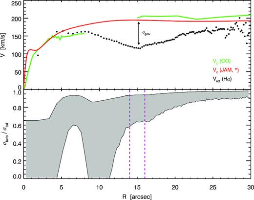
Top panel: Circular velocities derived from stellar dynamical modelling (red) and CO kinematics (green), allow for a decomposition of H α velocity dispersion into gravitational and turbulent components. Black points indicate the observed H α rotation curve, which we use in solving equation (2) to derive σgrav,H α. Bottom panel: Grey area shows the possible fraction of H α velocity dispersion which is turbulent in nature, with the range due to an uncertainty in velocity anisotropy. Magenta lines indicate the region of the σH α peak.
Shifting focus to the outer transverse dust shell, in the second from bottom left panel of Fig. 2, we show the distribution of the CO velocity dispersion (σCO). This can reach above 30 km s−1, but only in three localized regions: the galaxy centre; an expected peak at the southern entry/contact point between the nuclear ring and the bar dust lane; and at the southern portion of the transversal dust lane. The bottom left map in this figure shows the residual velocity field derived by subtracting the circular velocity profile from the observed CO velocity field. The south portion of the transversal dust lane shows projected deviations from circular velocity of approximately −40 km s−1. The detailed kinematics of this transverse CO shell deserve special attention. The northern half of the feature shows approximately zero residual velocity and very low velocity dispersion, the combination of which suggests that even in the presence of projection effects, this portion of the CO is no longer radially expanding outwards. In the southern portion of the transverse feature we see a discontinuity where the residual velocity field jumps to Vres ∼ −40 km s−1, with an associated peak in dispersion.
Due to inclination effects this decrease in residual velocity could result from a negative azimuthal peculiar velocity or a positive radial component (or a combination of both). However the northern part of the transverse shell agrees with the velocity expected from the global rotation curve. Given the geometry of the system (the east/left part of the galaxy must be the near side assuming that the main dust lanes appear on the leading side of the bar), if the motion that is causing this negative residual velocity is purely radial, and in the plane of the galaxy, then it can only be moving away from the galactic centre. It is interesting to note that the largest H α dispersions and radial flows are near this portion of the transverse dust shell.
Taken together in the context of our scenario for the shell evolution, the H α residual velocity and associated dispersion peak may partly arise from the outflowing ionized gas colliding with the slower moving (or stalled) CO shell – increasing the dispersion in both the CO and H α and inducing small additional radial motions in the southern portion of the transverse CO shell. We discuss further possibilities for the high-velocity dispersion, related to the confined outflow of the gas, in Section 6.4.
5 MODELLING THE STELLAR FEEDBACK AND OUTFLOW DYNAMICS
A zeroth order test of whether the stellar feedback in the nuclear ring could be responsible for the outflow comes from considering the kinetic energy of the outflowing gas relative to the energy of the starburst. Using the velocity field built from the Hα emission in the MUSE cube that we derived (Fig. 4), we have determined the speed that the warm gas is expanding radially from the nuclear ring, vrad ∼ 70 km s−1. Using the total H α luminosity, we inferred the total ionized gas mass in the cavity to be approximately Mion = 1.2 × 10⁶ M⊙ using equation 2 of Förster Schreiber et al. (2018). With these quantities we derive an order of magnitude estimate for the kinetic energy imprinted on the warm gas from the nuclear ring, finding |$E_{\rm kin} = 1/2 M_{\mathrm{ ion}}v_{\mathrm{ rad}}^{2} \simeq 6\times 10^{52}$| erg. As we shall see below this is approximately two orders of magnitude smaller than the energy provided by the stellar feedback in the nuclear star forming ring (within R ≲ 220 pc), and given that molecular gas mass in the shell is approximately half the gas mass in the cavity, suggests that even considering only energy input from the western side of the ring and a mechanical efficiency of a few per cent, stellar feedback could be responsible for the ionized outflow – and moving the transverse molecular gas feature from the ring, to its present location.
5.1 Feedback energetics
In order to estimate the energy budget from the star-forming nuclear ring of NGC 3351, we combine stellar population synthesis models (starburst99; Leitherer et al. 1999, hereafter SB99) with analytic prescriptions for momentum injection due to various stellar feedback mechanisms. The baseline SB99 models were run at solar metallicity, with a Kroupa IMF, and an SFR = 0.6 M⊙ yr−1 (which are the average observed metallicity and SFR in the ring derived from our MUSE observations). The models assume the SFR is constant over the relevant dynamical time-scales in this system (≲100 Myr). We use the energy budget and ionizing photon budget from these computations to model four feedback processes: SNe II, stellar winds, direct photon pressure, and photoionization heating. Below we describe the baseline model prescriptions, however systematic variations in the input to the SB99 models or in the subgrid feedback prescriptions are discussed in Appendix A.
5.1.1 SNe II
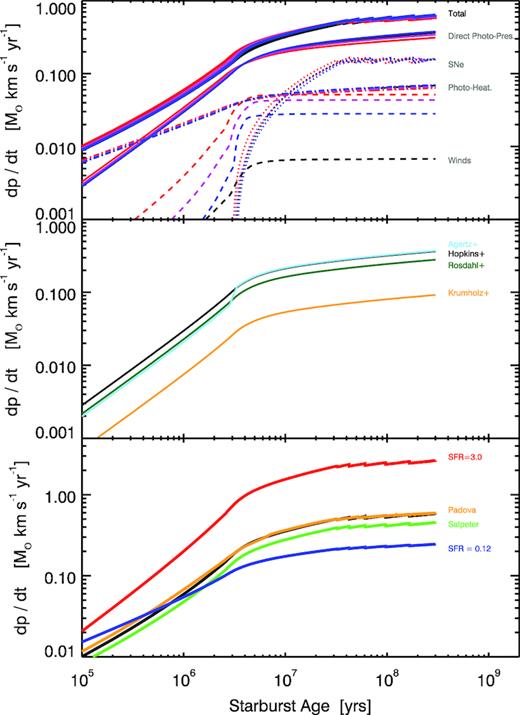
Variations in momentum flux due to different physical and sub-grid prescriptions. Top: Effect of metallicity changes (blue, Z = 0.008; magenta, Z = 0.020; red, Z = 0.040) primarily impact the stellar wind contribution. Middle: Effect of different sub-grid feedback prescriptions for direct photon pressure coupling and scattering in gas, used by various simulation groups (see Appendix A for details). Bottom: Effect of changing SFR in the ring, as well as using a stellar library which includes AGB winds (Padova), or using a Salpeter instead of Kroupa IMF.
5.1.2 Stellar winds
The energy, mechanical luminosities, and momentum flux of the stellar winds are output directly by the SB99 models, and account for radiation driven outflows from stars in post-MS evolutionary phases. These winds have a strong metallicity dependence as the radiation coupling will be more efficiently absorbed in the envelopes of metal rich stars. This effect can be seen clearly in Fig. 7 – however even with the high metallicity regime we see here, the winds from the stars is still sub-dominant.
5.1.3 Direct photon pressure
5.1.4 Photoionization heating
Fig. 7 shows the momentum flux for the four feedback sources. Under the framework of the parametrizations which we are using (which we have chosen to most closely match cosmological simulation prescriptions) direct momentum injection from the young massive stars ionizing radiation (∼τL/c) is the energetically dominant mechanism (40−60 per cent) of the four in this high metallicity regime. In what follows, given the nearly constant SFH derived for the ring (Appendix B) we utilize momentum flux values in the plateau regions of the curves in, e.g. Fig. 7.
5.2 Outflow expansion model
For the time being, as our the dynamical arguments and simulations suggest a non-gravitational origin of the transverse shell, we can use these models and now ask if, and over what time-scale, the observed feedback energetics can move the transverse shell of cold gas/dust from the nuclear ring to its current position.
Fig. 8 shows the time evolution of the dusty molecular gas shell, using the energy derived from the feedback modelling (primarily SNe, photoionization heating, and radiation pressure), in conjunction with simple bubble evolution models. In these illustrative test models the shell typically takes ∼107 yr to expand to its current location, though the three bottom panels in this figure show qualitatively how this changes with differences in the input SFR, surrounding ISM density, or dust opacity factor. The parametrization of the latter mimics multiple scattering events by photons which can boost the momentum deposition by radiation in a dusty ISM. We study the variation of this process, as multiscattering may be important for our system where the outflow velocities and optical depths are rather low (Costa et al. 2018).
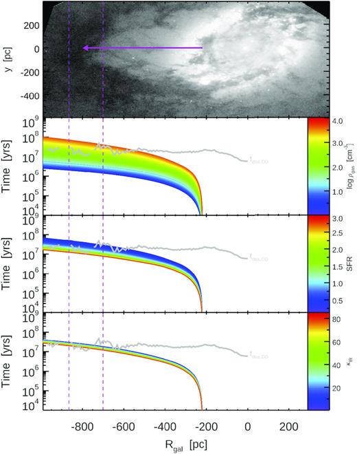
Feedback driven bubble evolution models for various initial gas densities (top panel), SFRs (middle panel), and dust opacity coefficients (κIR, bottom panel). The vertical dashed lines show the current location (DCO) of the primary dust/gas shell which has been blown out from the SF ring (travelling a distance of RCO). Bottom three panels show the time evolution of the shell for different model parameters (with the other two fixed to their median values). Grey lines show the observed turbulent energy dissipation time-scale for the CO gas at that radius – similar to the likely expansion time for the shell in NGC 3351.
To better characterize the expansion time and degeneracies in parameters setting the bubble dynamics, we run an MCMC analysis to ascertain if any qualitative constraints on the original SFR, gas density, metallicity, or opacity/re-scattering factor are possible. The last parameter in particular could be of help for modelling (sub-grid) feedback in modern hydrodynamical galaxy simulations where the softening length or smallest cell size of the simulation is approaching our MUSE spatial resolution (∼10 pc).
We draw parameters θ = (SFR, ρISM, Z, κIR) for each bubble expansion model from a uniform set of priors, which cover the physically expected range of these values in observed or simulated galaxies: −6 ≤ log SFR ≤ 6, −6 ≤ logρ ≤ 6, −3 ≤ log(Z) ≤ 0.7, and 0.1 ≤ κ ≤ 100. The SFR and metallicity set the energy budget output by the SB99 models, which with our feedback parametrizations, describe the effective work done on the shell by SNe, direct photon pressure, and subsequent photoionization heating. The shell is assumed to initially be at the location of the H α SF ring (Rinitial = 220 pc), embedded in a density ρISM. The range of sampled densities is chosen initially to be quite agnostic and spans values outside those observed for either the ionized or molecular gas in NGC 3351. The available energy from SNe, stellar winds, and direct photon pressure is then used as input along with the gas density to compute the time evolution of the dusty gas shell outwards, using the analytic bubble expansion model (equation 7).
For a given set of model parameters, each evaluation yields a time-scale (tstall) for the gas shell to travel to the observed present day location (DCO = 738 ± 127 pc), and how close the model makes it to that location (Dmax) (as some never pass that distance). The likelihood is computed taking into account the difference between the model metallicity, SFR and maximum distance, and those observed quantities (DCO = 738 ± 127 pc, SFR = 0.6 ± 0.3, Z/Z⊙ = 2 ± 0.5). To sample the distributions we use a modified idl implementation of emcee, originally developed for python by Foreman-Mackey et al. (2013), with 300 walkers running 1000 simulations each. The first 30 per cent of the trials are discarded in order to ensure the results are not dependent on the walker initialization. The posterior distributions for the four model parameters (SFR, ρISM, Z, and κIR) as well as the time when expansion crosses the observed location of the CO shell are shown in Fig. 9. Covariance plots between the model parameters are shown in Fig. C1 and are discussed in Appendix C.
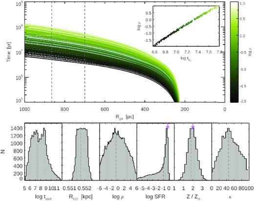
Posterior distributions from the MCMC analysis of our feedback driven shell expansion models (bottom row). Median and 1-σ confidence intervals are indicated as dashed and dotted lines for the parameters in the model (mean ISM density, SFR, metallicity, and dust opacity coefficient), as well as the recovered shell expansion time at the location of the shell (RCO). Observed SFR and metallicity values in the ring are marked as the magenta arrows. Top panel shows the distance evolution from the bubble expansion models for trials run for the observed range of densities in NGC 3351, with inset showing the ISM density dependence of the shell expansion time.
The top panel of Fig. 9 also shows some of the most likely bubble expansion models which reproduce the CO shell location. Here we have reproduced only models with densities spanned by the ionized and molecular gas observations in the galaxy. In these models the shell expands to its current location in a typical time-scale of log tstall = 7.2 ± 0.6 yr. Even for the limiting kinetic energy values seen in the hot gas (∼6 × 1052 erg), this implies a total power of up to 4.8 × 1038 erg s−1. The favoured initial density and metallicity are quite close to those derived from our observations, though the SFR is a factor of 1.5–6 lower than the integrated SFR in the Hα ring. However we measure the present day SFR over the full ring (not the half which impacts the outflow), and our derived SFHs (see Fig. 11 and Appendix C) suggest the SFR might have been lower in the past. It therefore appears that a stellar feedback origin for the transverse dust and CO shell is quantitatively supported by these simple models.
5.3 Initial Mass-loading Factors
Simulations of MW mass galaxies can show redshift zero mass-loading factors (|$\eta = \dot{M}_{\rm out}/\mathrm{ SFR}$|) of below unity, while at high redshift they may approach 10 (Muratov et al. 2015). Our combined feedback and outflow models yield the distance–time evolution of the shell, for a given model’s initial density and SFR. This provides all the necessary ingredients for an estimate of the initial mass-loading factor, which self-consistently powers the expansion of the shell to the current location. These are shown schematically as the coloured bands in Fig. 10 for different input SFRs in a model.
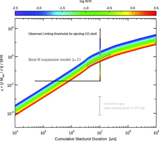
Mass-loading factor (mass outflow rate divided by SFR) as a function of time from the combined SB99, feedback and bubble evolution models (coloured lines). Shown as the grey error bar is the current mass-loading factor for the low density H α gas in the cavity between the CO shell and nuclear ring. Black solid line shows the necessary mass-loading factor that would have been required to initially eject the cold molecular gas shell from the ring to its observed present day position if the current outflow velocity is used. Dark grey polygon is the 1σ region from our best fit bubble expansion models.
A conservative estimate of the initial mass-loading factor can be taken from the observed molecular gas mass in the shell and a constant observed outflow velocity of 50 km s−1 (η ∼ (M × V/R)/(SFR)). This is indicated in Fig. 10 as black lines. We note that this conservative lower limit assumes a spherical outflowing geometry, while most of the molecular gas is concentrated in a shell. At the radius of the molecular gas shell, the mass-loading factor would have to be multiplied by Ωsph/Ωobs ∼ 3.5 with respect to the spherical analytic models in order to account for this geometrical difference.
From the shell expansion models, we can coarsely estimate the initial mass-loading factor at the time the shell was launched by considering the input SFR for the model, the total momentum flux of all feedback sources incident on the shell, and the model derived velocity at each point in time (η ∼ (dp/dt)/v(t)/SFR). This approximate estimate of the mass-loading factor assumes spherical symmetry for the long-term evolution of the shell through the ISM, but does not specify whether the shell was launched as a coherent entity, or swept up along the way – as the model is noted to be well tailored to simulations of a heterogeneous and clumpy ISM. The shell expansion models which fall within 1 − σ of the observed SFR (0.6 ± 0.3 M⊙ yr−1) suggest an initial mass-loading factor of 0.2 ≲ η ≲ 1.5 (grey parallelogram), similar to what is seen in simulations of z = 0 MW mass galaxies in literature (c.f. Schroetter et al. 2016). Reassuringly, these models lay within the permitted region on this diagram – providing a strong consistency check.
The initial mass-loading factor can be compared to observational estimates of the current mass outflow rate from the ring in NGC 3351 following equation 2 of Förster Schreiber et al. (2018). We compute this present day mass-loading factor locally in the ring using the current ionized gas mass, and the maximal observed radial component of the ionized gas velocity field (Vrad ∼ 70 km s−1). This instantaneous mass-loading factor for the ionized gas is well below unity (η0 ≤ 1.3 × 10⁻³), not surprising given its low density.
6 SURVIVAL AND FATE OF THE COLD GAS
While molecular and neutral gas streamers and shells have been observed in much larger, galactic-scale winds (e.g. Walter et al. 2017), the genesis of cold molecular gas in any energetic, ionized outflow is still debated. The cold gas is naively expected to be crushed by shocks or heated by conduction on time-scales much less than the outflow travel times. Here we consider three theoretical models for cold gas survival/formation in outflows in the context of the molecular shell which bounds the cavity of H α emission (S1 in Fig. 11), and which we interpret as having been initially pushed out by stellar feedback.
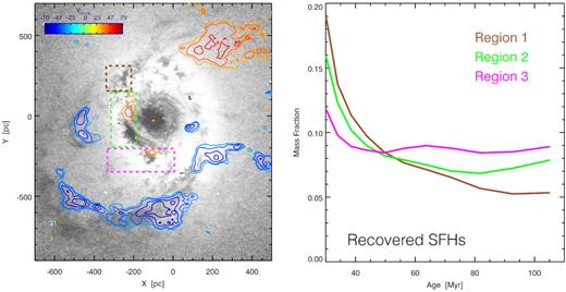
HST F555W–F814W grey-scale image (left) showing the primary dust shell (S1), as well as a smaller secondary dust feature (S2). The secondary shell has an associated ionized gas outflow kinematic signature (Vres,H α shown as coloured contours) and shows a distinct SFH (right).
6.1 In situ condensation
McCourt et al. (2018) recently posited that a cold component may condense in situ in the outflow if the warm ionized gas can shatter into droplets, which isobarically cool on short time-scales. The ratio of the cooling time to the crushing time for any cloud is proportional to the Mach number, |$t_{\rm cool}/t_{\rm crush} \propto \mathcal {M}$|. Therefore as our outflow is supersonic (|$\mathcal {M} \simeq 2$|; see Section 6.2), we do not expect this condensation to occur – and even if it did, the entrainment time (for the condensed gas to move with the hot flow) would be a factor of three longer than the crushing time (see Table 1). Thus both the survival of the gas and its entrainment are not likely to happen in the necessary time-scale to allow for in situ condensation of gas in this particular outflow. In addition, the authors note that this process should only help transition ionized gas to a neutral phase, and may not apply to supersonic, self-gravitating molecular gas. Post-shock cooling scenarios developed for molecular AGN outflows (c.f. King & Pounds 2015), require orders of magnitude higher shock velocities and cavity temperatures than seen here. Therefore we consider that in situ condensation is not a highly probably origin for the molecular gas shell in NGC 3351.
6.2 Radiative cooling
6.2.1 Independent estimates of the initial mass-loading factor
The critical mass loading and SFR surface density reported in equations (13) and (14) necessary for radiative cooling to dominate, are only marginally outside the range of the values of η from our bubble expansion models (e.g. the grey parallelogram in Fig. 10), and the SFR densities at peak locations in the ring (Fig. 5). Lacking more stringent constraints from that dynamical analysis and wishing to better understand whether radiative cooling could play a role in the outflow, we here explore two additional independent constraints on the mass-loading factor. The first is a theoretical estimate for the fraction of escaping mass in the outflow, and the second is a related observational estimate of the fraction of mass in our outflow which is above the escape velocity curve of the galactic potential – and both can be related to the initial mass-loading factor.
This independent constraint on η is an upper limit, as likely not all of the measured SFR couples energetically to the gas. Additionally the short conduction time suggests that the temperature structure within the inner part of the cavity will be homogenized efficiently (∼106 yr), perhaps inhibiting either cooling or condensation. Despite these, it is already below the critical mass-loading factor necessary to aid radiative cooling from the analysis in Section 6.2 (ηcrit ≥ 2.5). This then might suggest that a radiative cooling origin for the cold gas is plausible in general, but perhaps not occurring in NGC 3351 given the low SFR column densities and short travel time and distance.
This is confirmed if we directly ask what fraction of the H α flux in our MUSE observations is moving faster than the local escape velocity (as derived from our stellar dynamical modelling and independently confirmed via the CO circular velocity profile in Section 2.4). We find from the observations that only 5 × 10⁻⁵ of the total H α flux is moving faster than the local escape velocity. This corresponds to an escaping mass fraction of 3.7 × 10⁻⁴ ≤ ς ≤ 3.7 × 10⁻³ given the range of electron densities in the cavity (ne ∼ 102−3).
6.3 Magnetic entrainment
Finally we consider the survival of the molecular gas in the context of our favoured dynamical scenario (Section 1.1) – that the molecular gas was launched from the central ring primarily by direct photon pressure operating on the dust. The molecular gas can be aided in its survival during such an outflow, by the galaxy’s magnetic field lines (McCourt et al. 2015). These would initially be wound through the dusty ISM in the ring, and could prevent the molecular shell from disrupting as it is pushed out, while also inhibiting conductive heating.
McCourt et al. (2015) also note an indirect estimate of the stopping distance for the wind in this magnetic entrainment scenario can be computed as |$d_{\mathrm{ stall}} \sim R_{\mathrm{ cloud}}(\rho _{\mathrm{ cloud}}/\rho _{\mathrm{ wind}})(\beta _{\mathrm{ wind}}\mathcal {M}^{2})/(1 + \beta _{\mathrm{ wind}}\mathcal {M}^{2})$|. The relative Mach number of the cloud to the wind ranges from 1.9 to 5.3 for our flow, and from the best-fitting expansion models and equation (21) βwind ∼ 0.003. Using these along with the typical densities in our CO cloud and wind, we find dstall ∼ 150−1032 pc. The range of these expected stalling distances spans the observed present day travel distance of the CO shell (RCO ∼ 520 pc), however the large uncertainties only let us speculate that if the shell were indeed stalled, this may not be problematic for the magnetic entrainment scenario. It should be kept in mind that there are significant systematic uncertainties in these simple analytic predictions, due to geometry or other factors, which prevent a conclusive statement on the validity of this scenario.
Based on these simple calculations, a scenario where the cold gas/dust was aided in survival during its feedback driven outflow from the central ring by entrained magnetic fields appears possible. This is likely not a unique scenario, nor does it need to operate singularly. However this picture is consistent with our observations and energetic modelling of the outflow history (Section 3), and would reconcile the short conduction time-scales (tcond ∼ 106 yr) – which derived in the absence of magnetic fields, may be significantly less than in the presence of strong field lines (Thompson & Krumholz 2016).
The necessary magnetic field strengths (and orientation) for this scenario could perhaps be tested on this galaxy directly (or other comparable systems) with upcoming high resolution cm wavelength arrays, such as SKA – and indeed VLA and SOFIA-HAWC + observations of magnetic fields have already been demonstrated in several external galaxies (c.f. Beck 2015).
As a final summary, Table 1 shows several observed and derived relevant time-scales for the primary outflow feature in NGC 3351.
6.4 Geometry and fate of the outflow
At all radii the velocity dispersion of the ionized gas falls below the escape velocity of the galaxy, as derived from our JAM models and CO circular velocity curves; only a small fraction (∼10−4) is escaping the total potential of the galaxy.
As noted by Swartz et al. (2006), due to the inclination of NGC 3351 it is uncertain as to whether the outflow (observed in their study as X-ray emission in the cavity) is expanding spherically or within the plane. While naively one would expect expansion to be easier in the vertical direction, they suggest the outflow could be bounded in the plane of the disc – perhaps confined by ambient gas in a halo leftover from previous outflow events – though they could not fully rule out the possibility that the outflow is expanding vertically into the halo.
Swartz et al. (2006) did suggest that the planar component of the outflow is indeed confined radially by the transverse dust shell, as the X-ray emission is bounded by this feature – similar to the H α emission we observe. They further note that the unusual orientation of the dust lane with respect to the bar lane means that it could have been generated during the outflow event – consistent with the dynamical evidence presented here.
There are various analytic estimates of when a wind-driven outflow may breakout vertically from the plane of a galaxy. Using for example, the parametrization from the study of Mac Low & McCray (1988), we estimate the product of the mechanical luminosity and thermalization efficiency, |$\xi \dot{E}$|, to be a factor of ∼3–30 above their estimated threshold for breakout. This calculation assumes a isotropic outflow in a planar disc with scale height of H = 100 pc, and uses the luminosities and photoionization pressures from the SB99 and MUSE emission line diagnostics in the cavity. However the question of vertical confinement of gas is sensitive to the assumed scale height – for example a change to H = 200 pc results in no breakout. We note that assuming hydrostatic disc equilibrium (|$H = \sqrt{2}R\sigma _{\mathrm{ CO}}/V_{\mathrm{ CO}}$|) with our observed CO velocity dispersion favours H ∼ 200 pc at the current location of the shell – perhaps indicating the outflow has not expanded far out of the disc.
A vertically confined geometry is supported by considering the location and shape of the H α velocity dispersion peak in the outflow, relative to the peak of the radial outflow velocity and CO/dust shell. In Fig. 4 we can see: (1) a spatial offset between the velocity dispersion maximum and the leading edge of the outflow and (2) a similar curvature to the high velocity dispersion ionized gas, as that of the CO shell. Both provide clues to the geometry of the outflow. For an optically thin gas which is undergoing expansion from the central ring, we can ask where the maximum value in the projected line of sight velocity dispersion should be for (a) the case of a spherically expanding ionized gas cavity, and (b) a planar confined expansion.
Fig. 12 shows the projected LOS residual velocities, and the LOS H α velocity dispersion in the two outflow cases. While both residual velocity fields are consistent with our observations (by construction), only the vertically confined outflow model produces a well-defined peak in velocity dispersion behind the leading front of the outflow – in excellent agreement with the ∼150 pc observed offset between the σH α peak and the CO shell in Fig. 4. This gives support to the above analytic arguments for the outflow being partially confined in the vertical direction.
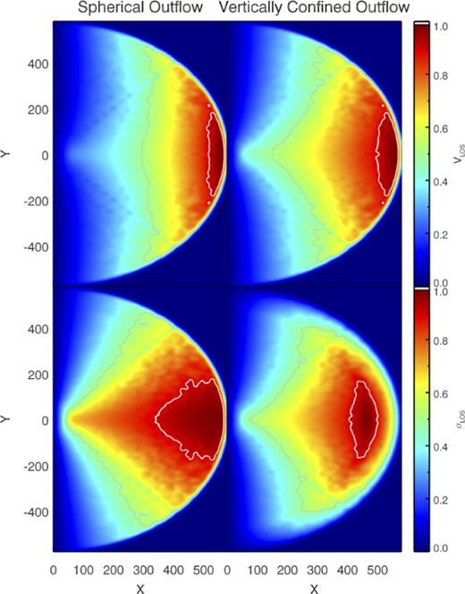
Top row: Radial component of the outflow velocity (projected on the sky) for an outflow that is spherically expanding (left), or vertically confined (right). Bottom row: The line-of-sight H α velocity dispersion in the two cases. The confined outflow model shows an peak in the velocity dispersion offset from the leading edge, in close agreement with our observed kinematics. All velocities are shown relative to the maximum value in the model velocity field, with the grey and white contours indicating levels at 50 and 90 per cent of the maximum.
Unlike some other systems in literature (e.g. Alatalo et al. 2011) which show outflow velocities greater than the escape velocity, NGC 3351 appears to have a small-scale nuclear outflow which can be powered by SF feedback and remain confined to the galactic potential.
7 DISCUSSION
The observed gas kinematics, feedback models, and simulations all imply that the transverse CO shell is not gravitational in nature, and that it is energetically feasible to have been ejected from the nuclear ring by stellar feedback. Subsequent sustained energy from SF in the ring could move the ionized low-density gas outwards in the cavity left behind, which we observe clearly as a radial component in the H α residual velocity map, orthogonal to the underlying galaxy velocity field.
While the scenario we present for the central region of NGC 3351 seems well supported by the data and our modelling, the unique boundary conditions from the multiphase ISM observations also offers an opportunity to address additional questions on galactic astrophysics.
7.1 Implications for feedback prescriptions in simulations
A result from our modelling of the dust shell expansion is that SNe alone cannot provide the necessary energy to move the bulk of the gas from the SF ring to its observed location. Indeed when we repeat the analysis of Section 3.2 with no direct photon pressure added to the energetics, we find that the shell expansion stops at roughly Rgal = 550 pc (dstall = 330 pc) for the same parameters.
While direct photon pressure is favoured as an additional energy source, we recover poor constraints on κ as a result of the density, metallicity and SFR dependence in the photon re-scattering parametrizations. This can be seen most clearly as an inflection in the ρ−SFR covariance plot in Fig. C1, as well as null correlations between κ and the other parameters in that figure. This unfortunately prevents us from the useful exercise of specifying an optimal κ to use as a function of an observables such as SFR.
Nevertheless, while κIR values favoured in our analysis may be difficult to directly compare to subgrid simulation prescriptions, it could be possible to gain insight to the differential behaviour of κIR by repeating the exercise in Section 3.2 for other galaxies with similar feedback driven gas flows. In this way perhaps relative changes in κ with respect to galaxy mass or peak SFR could be observationally studied.
The absolute values of κ spanned in the posterior distribution are larger than some currently implemented simulation prescriptions, however these values are potentially degenerate with an unconstrained level of fractal/inhomogeneous structure for the unresolved molecular medium.
In the meantime, given the complex systematics in how simulations implement radiation pressure, perhaps a better lever arm is to ask what type of simulated feedback can reproduce the observed expansion time, ionized outflow momenta, and emission line diagnostics – when using the same SFRs and gas densities as observed here? Can the morphology and dynamics of NGC 3351 be reproduced for a tailored simulation with feedback – and if so what prescriptions succeed or fail?
In particular, as magnetic entrainment may be important to the survival of the cold phase, the accounting of feedback simultaneously in the presence of magnetic fields should encourage new generations of simulations to incorporate magnetohydrodynamical processes.
7.2 Further questions
If the scenario presented here is a correct description of the dynamical evolution of the gas outside the nuclear star forming ring in NGC 3351, several consequences and questions emerge.
It would be interesting to understand how many other nuclear ring systems show similar morphology in the cold gas and dust in order to better characterize if there is a particular metallicity threshold necessary to efficiently eject these gas shells. Or alternatively characterize if there is a specific SFR density or cadence that is necessary to generate such features.
A census and characterization of such transverse features may be beneficial as they hold not only a record of the outflow and star formation burst time-scales in the galaxy, but also should provide a simple way of estimating the bar pattern speed.
From a chemical enrichment point of view, such large-scale radial gas motions may transport metals a significant distance in the inner regions of the galaxy (c.f. Gibson et al. 2013). Similarly, more energetic flows, or those occurring in less dense discs may break out in the vertical direction and transport metals via a ‘galactic fountain’ scenario. If discrete enough in time, both of these gas motions may also produce azimuthal variations in metallicity due to the bar and ring rotation – relevant in light of some studies finding variations in the abundances of spiral (inter)arm regions of galaxies (Ho et al. 2017).
Understanding the dynamics and energetics associated with these non-gravitational features in the gas will hopefully lead to improvements in our understanding of stellar feedback’s impact on the ISM in local galaxies and simulations.
8 SUMMARY AND CONCLUSIONS
We have used MUSE, ALMA, and HST observations of a transverse dust and molecular gas shell, located at the leading edge of an ionized gaseous outflow emanating from the central star-forming galactic ring in NGC 3351, to self-consistently describe its morphology and dynamics due to observable stellar feedback. Our key results are as follows:
By running hydrodynamic gas response simulations with the derived gravitational potential of NGC 3351, we see that the observed transverse dust lane is likely not due to the underlying non-axisymmetric gravitational potential. As such, additional processes related to SF and stellar feedback are necessary to explain the presence and location of the transverse CO gas shell.
From the observed SFRs in the nuclear ring, we model the total momentum flux incident on the molecular gas shell using starburst99 models and analytic feedback prescriptions. We find that based on the total momentum flux incident on the molecular gas shell, the dominant source of momentum injection is from direct photon pressure (|$\sim 40\!-\!60$| per cent), with SNe (|$\sim 20\!-\!30\,\mathrm{ per}\,\mathrm{ cent}$|), photoionization heating (|$\sim 10\!-\!15$| per cent), and stellar winds (|$\sim 1\!-\!10$| per cent) progressively less important.
Dynamical modelling of the outflow, suggests the dusty, cold molecular gas was initially driven from the nuclear ring by SNe and radiation pressure, with an initial mass-loading factor of η ∼ 0.1, and took approximately 107 yr to reach its current location. This expansion time is close to the turbulent dissipation time of the molecular gas in the transverse shell at present.
Concurrent star formation powered strong radial outflows of low density ionized gas, which we observe in the MUSE H α residual velocity field to have Vrad ∼ 70 km s−1, and cross orthogonally to the underlying circular orbits of the galactic velocity field. This, and their confinement by the molecular gas shell, leads to visible shocks in the warm cavity bounded by the nuclear ring and dust shell. The emission line diagnostics and velocities in this cavity are in agreement with predictions from fast-shock models.
The geometry of the dust and ionized gas outflow is consistent with magnetic fields providing a (protective) drag force on the molecular gas in the outflow during its initial ejection by feedback from the nuclear ring. In situ condensation and radiative cooling of the molecular gas are less likely for this system, as implied by the short dynamical time-scale and low mass-loading factors.
Comparison of the Hα kinematics to the galaxy escape velocity profile, indicates that the outflowing gas will not escape the galaxy potential.
The morphology of the ionized gas velocity dispersion field relative to the outflow front, is most consistent with a vertically confined outflow, with an opening angle of ∼30°, suggesting it has not significantly broken out of the disc plane.
The corresponding power generated by the star formation may be as high as 5 × 1038 erg s−1. This is of order of half that found in low-luminosity AGN (see Cheung et al. 2016, and references therein). This provides at least one example that stellar feedback processes can imprint significant amounts of energy into the ISM even in galaxies showing no AGN activity. Stellar feedback can likely to be an important driver of gas motions in high redshift systems where the SFR is larger than local systems, regardness of whether they have an AGN.
NGC 3351 shows quantifiable evidence of SF impacting the bulk (cold) gas motions in the disc plane, which has consequences for understanding outflows and feedback in galaxies.
If such nuclear SF episodes produce Kpc scale molecular outflows even without AGN, it may become non-trivial to distinguish the relative contributions of the two sources if AGNs are also present in partially resolved systems. If molecular gas can be kept cool due to magnetic fields in the ISM, how frequent is this also in cold gas AGN-driven outflows? The importance may be two-fold if the feedback momentum injection is also altered by the presence of magnetic fields. These can both be addressed by continued advancements of MHD in simulations (e.g. Marinacci et al. 2017; Pakmor et al. 2017).
Observationally, an increased joint census of the molecular gas content in nearby starburst galaxies and direct measurements of their magnetic field strength with present and future cm wave interferometric facilities will provide significant constraints for theoretical understanding of the interplay between feedback and magnetic fields. Similar analyses as presented here, applied differentially to other galaxies with joint molecular and ionized gas observations, may lead to more helpful constraints for sub-grid prescriptions of stellar feedback in modern galaxy formation simulations, the survival and entrainment of cold gas in outflows, and a better understanding of the time-scales for nuclear ring formation and evolution.
ACKNOWLEDGEMENTS
We thank the anonymous referee for an extremely helpful referee report which greatly improved this manuscript. The authors thank Morgan Fouesneau, Eva Schinnerer, Trevor Mendel, Thorsten Naab, I-Ting Ho, Rebecca McElroy, Alessandra Mastrobuono-Battisti, Chiara Mazzucchelli, Sebastien Viaene, Mattia Sormani, and Naomi McClure-Griffiths for useful discussions which helped improve this manuscript. This work was supported by Sonderforschungsbereich SFB 881 ‘The Milky Way System’ (subproject A7 and A8) of the Deutsche Forschungsgemeinschaft (DFG), and was also made possible with funding from the Natural Sciences and Engineering Research Council of Canada PDF award. RL thanks AH. Based on observations collected at the European Organisation for Astronomical Research in the Southern Hemisphere under ESO programme 097.B-0640(A). RL, GvdV, AdL-C, and JF-B acknowledge support from grant AYA2016-77237-C3-1-P from the Spanish Ministry of Economy and Competitiveness (MINECO). PS-B acknowledges support from grant AYA2016-77237-C3-2-P. GvdV acknowledges funding from the European Research Council (ERC) under the European Union’s Horizon 2020 research and innovation programme under grant agreement no. 724857 (Consolidator Grant ArcheoDyn).
Footnotes
This function, which has the form ftape(r) = exp((r − r1)2)/(2d2) smoothly truncates the gaseous disc for r > r1, in order to avoid density discontinuities or numerical issues at the boundary of the simulation box.
For more details on this process see section 4 of Fragkoudi et al. (2017).
REFERENCES
APPENDIX A: SIMULATION SUB-GRID FEEDBACK PRESCRIPTIONS
While the SNe momentum flux, and wind momentum flux are directly output from the SB99 models, the direct photon-pressure momentum flux, depends not only on that output ionizing luminosity, but also on a prescription for how the photons may interact, re-scatter, or become trapped within the dusty cold gas.
The baseline models for radiation pressure we adopt in the MCMC analysis of NGC 3351, come from Hopkins et al. (2014, 2017), which parametrize the opacity and (possible extra scattering) with a density and metallicity dependent factor – whereby more dense and metal rich gas should more effectively harness the momentum from the ionizing photons.
To understand systematics on this, Fig. 7 illustrates systematic differences in the sub-grid prescriptions for radiative pressure used in several high resolution hydrodynamical galaxy formation simulations, which we describe below.
A1 Hopkins et al.
A2 Rosdahl et al.
Rosdahl et al. (2015) follow a similar formalism to Hopkins et al., but with an opacity factor κ, which varies as a function of wavelength from κIR = 10(Z/Z⊙) to κopt,UV = 1000(Z/Z⊙). To illustrate the quantitative effect of the variation in κ, we show the difference in expansion time-scales for the dusty CO shell in Fig. 8.
A3 Agertz et al.
Agertz et al. (2013) allow for both a variation in the opacity and re-scattering coefficient, depending on if the radiation pressure acts on a time-scale larger or shorter than a typical self-bound molecular cloud. As seen in Fig. 7, the transition between these two regimes, nicely bounds the baseline models from Hopkins et al. (2014) and Rosdahl et al. (2015).
The baseline model of Agertz et al. (2013) that we adopt has the parameters: κIR = 5(Z/Z⊙), μmax = 1, tcloud = 3 Myr, η1 = η2 = 2, α = 0, β = 1.7, CR = 2.5, Mmin = 100 M⊙, and ϵcloud = 0.2. We run these assuming the maximum stellar mass (from the S4G mass maps; Querejeta et al. 2015) in the ring is Mmax = 107 M⊙.
A4 Krumholz et al.
For NGC 3351, the observed luminosities, SFRs and gas densities give maximal values of (τ, fE, ftrap) ≃ (0.004, 0.03, 0.002), indicating we are still in a low SF regime for these models.
As noted by Krumholz & Thompson (2012), even in higher SFR surface density regimes, the effective trapping is lower in their models than in the Hopkins et al. (2014) prescriptions, which can be seen quantitatively for the application of the models to NGC 3351 in Fig. 7.
APPENDIX B: STAR FORMATION HISTORY OF NGC 3351’S NUCLEAR RING
The MUSE spectra contain a wealth of information on the stellar populations within NGC 3351. To recover the recent SFH in different regions of the central ring in NGC 3351 we use the full spectral fitting routine steckmap (STEllar Content and Kinematics via Maximum a Posteriori; Ocvirk et al. 2006b,a). The justification and testing of this methodology is outlined in e.g. Sánchez-Blázquez et al. (2011), Ruiz-Lara et al. (2015), and our adopted methodology is described in detail in Sánchez-Blázquez et al. (2014). In short, the integrated spectrum within a given spaxel is compared to a grid of composite stellar population models in order to recover the light weighted mass fractions in different age bins. This is a non-parametric method for recovering the SFH and does not impose any particular shape for the solutions.
The SFH analysis utilizes the models from Vazdekis et al. (2010), which have been computed with the MILES stellar library (Sánchez-Blázquez et al. 2006; Cenarro et al. 2007). The SFH is inferred from the spectral fits, after first fixing the kinematic parameters (σ, Vsys) with pPXF (Cappellari 2017), correcting for instrument response and extinction effects to the stellar continuum, and masking emission lines and sky residuals.
Fig. 11 shows the derived mass fractions as a function of time (SFH) in the last 120 Myr for three regions in the star forming central ring. The left hand panel shows a map of the central region of NGC 3351, in which the primary dust shell is clearly seen (labelled S1), however in addition a smaller dust shell (S2) is also visible. This secondary shell shows an associated kinematic outflow in the Hα residual velocity field, stellar feedback from the ring has occurred discretely in time, and powered multiple outflow events.
While the age limits (tmin = 30 Myr) of the stellar library prevent a firm link between the recent SF of the ring and any morphological features, it appears likely that the peak SFR in the ring occurred sometime in the last 30 Myr, consistent with the dynamical analysis presented in the subsequent section.
The first order result from the SFH analysis of the ring is that there is a coherent SFH across the ring, at least on time-scales of a few hundred Myr. This can be seen in Fig. B1 which shows the SFR in different age bins as a function of azimuthal sector in the ring. While there is a mild phase shift for the youngest age bin, the well matched curves would suggest that SFR variations in the ring are likely driven by the large scale fuelling of the ring via the feeding arms. This is perhaps not surprising if azimuthal variations were created (and erased) on the orbital time-scale of stars in the ring (∼10 Myr), which is below the age resolution of our youngest SFH bin.
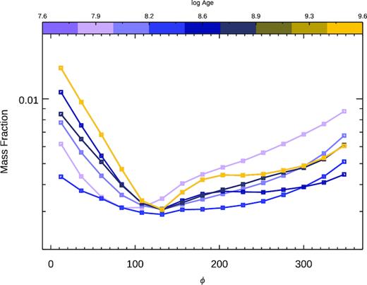
Mass fraction in different age bins, as a function of azimuthal angle in the ring (ϕ = 0 is aligned with North on the galaxy image). There is perhaps a mild phase shift in the minimum for the youngest age bins, but as a whole, to first order the ring SFH appears relatively coherent on these time-scales.
Smaller correlations amongst the various azimuthal sectors are visible as a very mild second order effect in Fig. B2, which shows the full SFHs and power spectrum of the SFHs as a function of azimuthal sector. For example, the sectors at opposing contact points (cyan/light blue versus orange) show consistently separated tracks in the power spectrum diagnostic, though the behaviour is mild, as indicated by the lack of visible trend in the bottom panel.
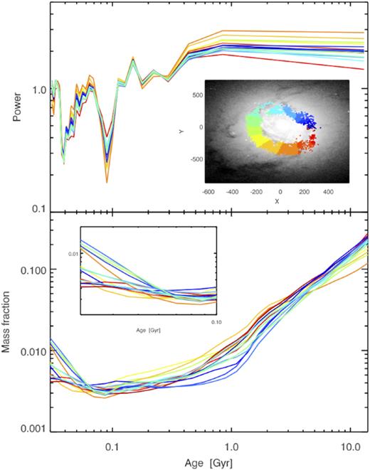
Power spectrum of the SFHs in different azimuthal sectors in the ring. There is a mild secondary effect with sectors nearest opposite contact points (orange, light blue) showing offset power at fixed period. Bottom panel shows the SFHs for all sectors.
APPENDIX C: COVARIANCE DIAGNOSTICS FOR THE FEEDBACK MODELS
For completeness, Fig. C1 shows the parameter correlations from the feedback model MCMC runs in Section 3.2.
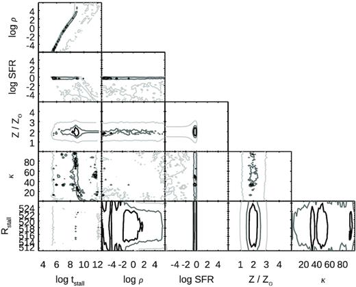
Covariance diagrams for the shell expansion model parameters. The density and metallicity dominate the final expression for momentum flux in the radiation pressure expression we use (Appendix A) and this as a consequence prevents useful constraints on κ.
APPENDIX D: MODEL VELOCITY FIELD SETUP
To construct the line of sight velocity dispersion maps for an optically thin expanding outflow, we consider integration of the underlying 3D velocity field along a sightline, in one of two underlying geometries: spherical outflow, or a vertically confined outflow. The intrinsic velocity field is defined in both geometries as V(R, θ, ϕ) = V0Rexp(R/Rshell), where θ is the azimuthal angle in the X−Y plane and ϕ the polar angle.
D1 Spherical outflow
Fig. D1 shows the geometry of an arbitrary sightline which strikes the spherical outflow at a projected galactocentric distance of |$R^{^{\prime }}$|, in a galaxy that is at distance Dgal from the observer, seen at inclination i.
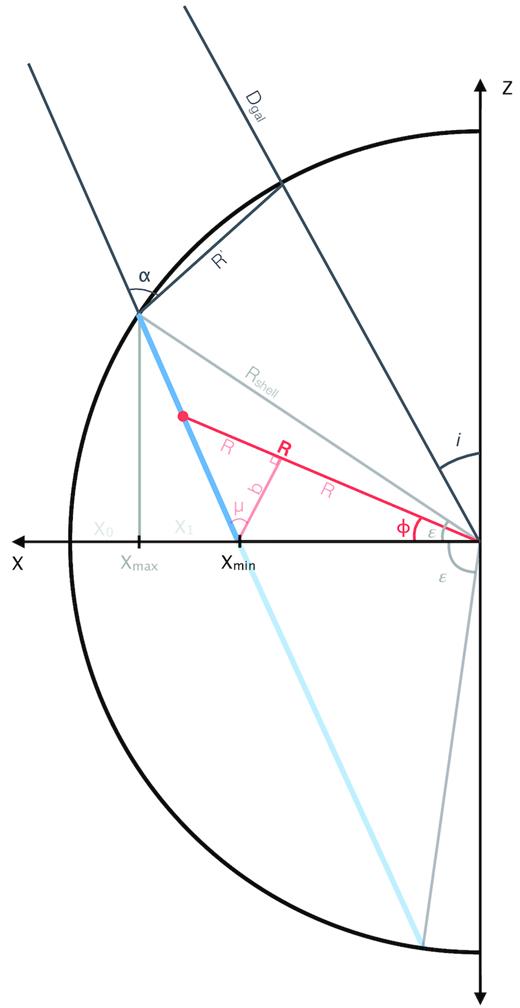
Geometry of line of sight through a spherical outflow of optically thin gas, in a galaxy seen at inclination i, here shown in the X–Z plane.
The line of sight can be parametrized by an angle from the plane of the galaxy ϵ. To parametrize the location along the line of sight through the velocity field (blue segment in Fig. D1), we consider a vector from the origin to a distance R, with angle ϕ. As ϕ sweeps from 0 ≤ ϕ ≤ ϵ, R corresponds to the 3D distance from the origin at that point on the line of sight segment.
The sign of the last argument is negative for the portion of the line-of-sight segment above the Z plane of the galaxy (e.g. 0 ≤ ϕ ≤ ϵ), and positive for the portion corresponding to ϵ− ≤ ϕ ≤ 0.
The sign of the term will change depending on if ϕ is above or below the plane of the galaxy. With this, the projected line-of-sight velocity dispersion is computed as the second moment of the integral in equation (E1).
D2 Vertically confined outflow
We next consider the case of an outflow confined in the vertical direction, with some critical opening angle ϕmax = arctan(Rcurve/Roff), which is defined by a radius of curvature for the confined outflow, relative to the maximum radial extent of the outflow Roff = Rshell − Rcurve. The geometry in the X–Z plane is similar to that of an ice-cream cone and is shown in Fig. D2.
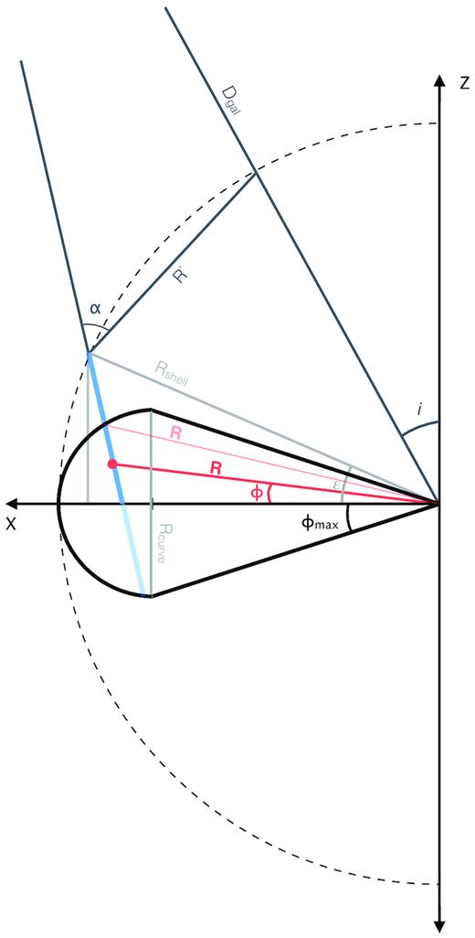
Geometry of line of sight through a vertically confined outflow of optically thin gas, in a galaxy seen at inclination i, here shown in the X–Z plane.
