


ABSTRACT
We present a general method to compute the non-linear matter power spectrum for dark energy (DE) and modified gravity scenarios with per cent-level accuracy. By adopting the halo model and non-linear perturbation theory, we predict the reaction of a lambda cold dark matter (ΛCDM) matter power spectrum to the physics of an extended cosmological parameter space. By comparing our predictions to N-body simulations we demonstrate that with no-free parameters we can recover the non-linear matter power spectrum for a wide range of different w0–wa DE models to better than 1 per cent accuracy out to k ≈ 1 |$h \,{\rm Mpc}^{-1}$|. We obtain a similar performance for both DGP and f(R) gravity, with the non-linear matter power spectrum predicted to better than 3 per cent accuracy over the same range of scales. When including direct measurements of the halo mass function from the simulations, this accuracy improves to 1 per cent. With a single suite of standard ΛCDM N-body simulations, our methodology provides a direct route to constrain a wide range of non-standard extensions to the concordance cosmology in the high signal-to-noise non-linear regime.
1 INTRODUCTION
General relativity (GR) has been put under intense scrutiny in the Solar system, where it has successfully passed all tests (Will 2014). Its application to cosmology, however, involves vastly different length-scales and is comparable in orders of magnitude to an extrapolation from an atomic nucleus to the scale of human experience. It is therefore important to perform independent tests of our theory of gravity in the cosmological regime. Further motivation for a thorough inspection of cosmological gravity can be drawn from the necessity of a large dark sector in the energy budget of our Universe to explain large-scale observations with GR (Riess et al. 1998; Perlmutter et al. 1999; Hildebrandt et al. 2017; Abbott et al. 2018; Aghanim et al. 2018). In particular the late-time accelerated expansion of the cosmos has traditionally been an important driver for the development of alternative theories of gravity, a concept that has, however, become strongly challenged with the confirmation of the luminal speed of gravity (Lombriser & Taylor 2016; Abbott et al. 2017b; Baker et al. 2017; Creminelli & Vernizzi 2017; Lombriser & Lima 2017; María Ezquiaga & Zumalacárregui 2017; Sakstein & Jain 2017; Battye, Pace & Trinh 2018; Creminelli et al. 2018; de Rham & Melville 2018). Nevertheless, cosmic acceleration could be the result of a dark energy (DE) field permeating the Universe that may well be coupled to matter with an observable impact on cosmological scales. Importantly, should that coupling be universal, i.e. affecting baryons and dark matter equally, the corresponding models must then rely on the employment of screening mechanisms to comply with the stringent Solar system bounds (Vainshtein 1972; Khoury & Weltman 2004; Babichev, Deffayet & Ziour 2009; Hinterbichler & Khoury 2010). Signatures of screening are naturally to be expected in the non-linear cosmological small-scale structure, where modified gravity transitions to GR, and for some models are even exclusively confined to these scales (Wang, Hui & Khoury 2012; Heymans & Zhao 2018). The increasing wealth of high-quality data at these scales (Laureijs et al. 2011; LSST Dark Energy Science Collaboration 2012; Hildebrandt et al. 2017; Abbott et al. 2018) renders cosmological tests of gravity a very timely enterprize. At the same time, cosmological structure formation proves notoriously difficult to model to sufficient accuracy in this regime, where high-signal-to-noise measurements have the potential to distinguish a few per cent deviation from GR (Heymans & Zhao 2018).
For any given theory of gravity or DE model, our current best predictions for the statistical properties of the resulting matter distribution come from large-volume high-resolution N-body simulations (Oyaizu 2008; Schmidt 2009b; Zhao, Li & Koyama 2011; Baldi 2012; Brax et al. 2012; Li et al. 2012; Barreira et al. 2013; Puchwein, Baldi & Springel 2013; Wyman, Jennings & Lima 2013; Li et al. 2013b; Llinares, Mota & Winther 2014; Winther et al. 2015). Running these, however, can take up to thousands of node-hours on dedicated cluster facilities, and although methods to partially alleviate this drawback exist (see e.g. Barreira, Bose & Li 2015; Mead et al. 2015a; Bose et al. 2017; Llinares 2017; Valogiannis & Bean 2017; Winther et al. 2017) exploring vast swathes of the theory space remains currently unfeasible. Alternatively, analytical and semi-analytical methods can be used to swiftly predict specific large-scale structure observables, such as the matter power spectrum (Koyama, Taruya & Hiramatsu 2009; Schmidt et al. 2009; Schmidt, Hu & Lima 2010; Li & Hu 2011; Fedeli, Dolag & Moscardini 2012; Brax & Valageas 2013; Lombriser, Koyama & Li 2014; Zhao 2014; Barreira et al. 2014a, b; Achitouv et al. 2016; Mead et al. 2016; Aviles & Cervantes-Cota 2017; Bose et al. 2018; Cusin, Lewandowski & Vernizzi 2018; Hu, Liu & Cai 2018), with the important caveat that they have limited accuracy in the non-linear regime of structure formation, and often involve some level of fitting to the same quantity measured in simulations. These approaches are therefore inadequate for future applications to high-quality data from Stage IV surveys (Laureijs et al. 2011; LSST Dark Energy Science Collaboration 2012; Levi et al. 2013; Koopmans et al. 2015), where per cent level accuracy over a wide range of scales will be necessary to obtain tight and unbiased constraints on departures from GR (Alonso et al. 2017; Casas et al. 2017; Reischke et al. 2018; Spurio Mancini et al. 2018; Taylor, Bernardeau & Kitching 2018b) and the nature of DE (Albrecht et al. 2006). Matter power spectrum emulators can provide a solution to this problem for particular modified gravity or DE models (Heitmann et al. 2014; Lawrence et al. 2017; Euclid Collaboration 2018; Winther et al. 2019), but still rely on the availability of large quantities of computational resources to determine the properties of the matter power spectrum at the location of the emulator nodes. The absence of a clear attractive alternative to the ΛCDM paradigm calls for a more general framework, one easily adaptable to non-standard cosmologies beyond the handful of well-studied cases.
Here we take an important step in this direction by extending the method proposed in Mead (2017), where the halo model is used to compute matter power spectrum ratios with respect to a convenient baseline cosmology. Mead (2017) showed that by determining these ratios, rather than the absolute value of the matter power spectrum, the shortcomings of the halo model are mitigated. The initial conditions of the baseline cosmology are designed so that under GR + ΛCDM evolution the linear clustering of matter at some given redshift exactly reproduces that of the target cosmology of interest, whose evolution is instead governed by non-standard laws of gravity and/or background expansion. Assuming one can generate an accurate non-linear matter power spectrum for the reference cosmology (e.g. with a suitable emulator), recovery of the target power spectrum then hinges on the computation of a ‘correction’ factor that incorporates the non-linear effects of fifth forces, screening mechanisms, and deviations from the cosmological constant. We use the halo model and non-linear perturbation theory to obtain such corrections, and refer to this quantity as the reaction.
The paper is organized as follows. In Section 2 we briefly describe popular modified gravity and DE models used here as test beds for our methodology. Section 3 reviews the halo model formalism and introduces the matter power spectrum reactions. The cosmological simulations used to validate our approach are described in Section 4, and Section 5 presents the capability of the halo model reactions to predict the non-linear matter power spectrum. We summarize our conclusions in Section 6. We provide details of the spherical collapse and perturbation theory calculations employed in this work in Appendices A and B, respectively. Additional tests to gauge the importance of the halo mass function and halo concentration in our predictions are presented in Appendix C.
2 DARK ENERGY AND MODIFIED GRAVITY THEORY
2.1 f(R) gravity
2.2 DGP
In the following we will consider the medium and weak nDGP variants used in Barreira, Sánchez & Schmidt (2016), with crossover scales rcH0 = 0.5 (nDGPm) and rcH0 = 2 (nDGPw) in units of the present-day Hubble horizon |$H_0^{-1}$|. Note that, at present, of these two cases nDGPw is the only one compatible with growth rate data (Barreira et al. 2016). Hence, similarly to F5, the use of nDGPm will serve as a test bed for our methodology in conditions of relatively strong departures from GR.
2.3 Dark energy
Table 1 summarizes the DE models selected for this work, which have been chosen to roughly enclose the 2σ region of parameter space allowed by the Planck 2015 temperature and polarization data in combination with baryon acoustic oscillations, supernova Ia, and H0 measurements (Planck Collaboration XIV 2016).
Equation-of-state parameters defining the DE models used in this work.
| Model | w0 | wa |
|---|---|---|
| DE1 | −0.7 | 0 |
| DE2 | −1.3 | 0 |
| DE3 | −1 | 0.5 |
| DE4 | −1 | −0.5 |
| DE5 | −0.7 | −1.5 |
| DE6 | −1.3 | 0.5 |
| Model | w0 | wa |
|---|---|---|
| DE1 | −0.7 | 0 |
| DE2 | −1.3 | 0 |
| DE3 | −1 | 0.5 |
| DE4 | −1 | −0.5 |
| DE5 | −0.7 | −1.5 |
| DE6 | −1.3 | 0.5 |
3 MATTER POWER SPECTRUM REACTION
In Sections 3.1 and 3.2 we briefly review the spherical collapse model and the halo model formalism, which we use to predict the non-linear matter power spectrum for the range of cosmological models listed in Section 2. The halo model assumes that all matter in the Universe is localized in virialized structures, called haloes. In this approach, the spatial distribution of these objects and their density profiles determine the statistics of the matter density field on all scales. It is typically assumed that each mass element belongs to one halo only, i.e. haloes are spatially exclusive. Below we introduce the ingredients entering the halo model prescription, and refer the interested reader to the Cooray & Sheth (2002) review on the topic for more details. In Section 3.3 we then detail our new approach to reach per cent level accuracy on these power spectra over a range of scales where the halo model alone is known to fail.
3.1 Spherical collapse model
3.2 Halo model
3.3 Halo model reactions
The apparent simplicity and versatility of the halo model has contributed to its widespread use as a method to predict the non-linear matter power spectrum in diverse scenarios. Examples include the ΛCDM cosmology (Peacock & Smith 2000; Seljak 2000; Giocoli et al. 2010; Valageas & Nishimichi 2011; Valageas, Nishimichi & Taruya 2013; Mohammed & Seljak 2014; Seljak & Vlah 2015; van Daalen & Schaye 2015; Mead et al. 2015b; Schmidt 2016), DE and modified gravity models (Schmidt et al. 2009, 2010; Li & Hu 2011; Fedeli et al. 2012; Brax & Valageas 2013; Lombriser et al. 2014; Barreira et al. 2014a, b; Achitouv et al. 2016; Mead et al. 2016; Hu et al. 2018), massive neutrinos (Abazajian et al. 2005; Massara, Villaescusa-Navarro & Viel 2014; Mead et al. 2016), baryonic physics (Fedeli 2014; Fedeli et al. 2014; Mohammed & Seljak 2014; Mead et al. 2015b), alternatives to cold dark matter (Dunstan et al. 2011; Schneider et al. 2012; Marsh 2016), and primordial non-Gaussianity (Smith, Desjacques & Marian 2011). Its imperfect underlying assumptions are however responsible for inaccuracies that limit its applicability to future high-quality data (see e.g. fig. 1 in Massara et al. 2014), where per cent level accuracy is required in order to obtain unbiased cosmological constraints (Huterer & Takada 2005; Eifler 2011; Hearin, Zentner & Ma 2012; Taylor, Kitching & McEwen 2018a).
To mitigate these downsides one can add complexity to the model at the expense of introducing new free parameters (see e.g. Seljak & Vlah 2015), fitting the existing ones to the matter power spectrum measured in simulations (see e.g. Mead et al. 2015b), or sensibly increasing the computational costs by going beyond linear order in perturbation theory (see e.g. Valageas & Nishimichi 2011). Here, instead, we follow and extend the approach presented in Mead (2017), which we shall refer to as halo model reactions.8
On large linear scales |$\mathcal {R} \rightarrow 1$| by definition;10
On small non-linear scales |$\mathcal {R} \approx P_{1\rm h}^{\rm real}/P_{1\rm h}^{\rm pseudo}$|;
Quasi-linear scales |$0.01 \lesssim k \, {\rm Mpc}\, h^{-1}\lesssim 0.1$| are well described by perturbation theory, while intermediate scales |$0.1 \lesssim k \, {\rm Mpc}\, h^{-1}\lesssim 1$| are primarily controlled by the halo mass function ratio |$n_{\rm vir}^{\rm real}/n_{\rm vir}^{\rm pseudo}$|.
Fixing the real and pseudo linear power spectra to be identical (as in equation 51) forces the corresponding mass functions to be somewhat similar. Therefore, owing to (iii), reaction functions can overcome the typical inaccuracies that plague the halo model in the transition region between large and small scales.
The role of the two-halo correction factor in equation (53) becomes clear in the limiting case k⋆ → ∞, where it goes to unity. Mead (2017) showed that this form of the reactions matches smooth DE simulations at per cent level or better on scales k ≲ 1 |$h \, {\rm Mpc}^{-1}$|for z = 0 (see also Section 5 below). On quasi-linear scales this remarkable agreement can be understood in terms of SPT. Schematically, the non-linear matter power spectrum is a non-trivial function of the linear power spectrum obtained through some operator |$\mathcal {K}$|, i.e. |$P(k) = \mathcal {K}[P_{\rm \scriptscriptstyle L}(k)]$| (Bernardeau et al. 2002). Provided that gravitational forces remain unchanged, then equation (51) enforces Preal ≈ Ppseudo on linear and quasi-linear scales. This is no longer true for modifications of gravity, since the structure of the |$\mathcal {K}_{\rm MG}$| operator is altered by different mode-couplings and screening mechanisms. We correct for this fact by including the two-halo pre-factor in equation (53), so that finite k⋆ roughly encapsulates the extent of the mismatch between |$\mathcal {K}_{\rm MG}$| and |$\mathcal {K}_{\rm GR}$|. For comparison, in F5 at z = 0 we have k⋆ = 0.3 |$h \, {\rm Mpc}^{-1}$|, whereas in nDGPm it becomes k⋆ = 0.95 |$h \, {\rm Mpc}^{-1}$|, which reflects the different screening efficiency on large scales between the chameleon and Vainshtein mechanisms.
Although our choice of k0 is commonly regarded as well within the quasi-linear regime, screening mechanisms in modified gravity induce non-linearities on large scales that can be more important than in GR. For this, the determination of k⋆ can be complicated by inaccuracies specific to the perturbation theory employed, and to reduce their impact on the halo model reactions we take advantage of the following two facts: (i) on large scales we expect |$P_{\rm NoScr}^{\rm real} \approx P^{\rm pseudo}$|, where |$P_{\rm NoScr}^{\rm real}$| denotes the non-linear matter power spectrum of the real cosmology assuming there is no screening mechanism; (ii) the kernel operators |$\mathcal {K}_{\rm MG}^{\rm Scr}$| and |$\mathcal {K}_{\rm MG}^{\rm NoScr}$| for the screened and unscreened real cosmology, respectively, have a similar structure (see Appendix B). Therefore, at least in principle, the ratio |$P_{\rm Scr,SPT}^{\rm real}/P_{\rm NoScr,SPT}^{\rm real}$| could give a better description of the reaction on large scales than the obvious candidate |$P_{\rm Scr,SPT}^{\rm real}/P_{\rm SPT}^{\rm pseudo}$|. Hereafter we will use |$P_{\rm NoScr,SPT}^{\rm real}$| instead of |$P_{\rm SPT}^{\rm pseudo}$| in equation (55), which in spite of being a sub-optimal strategy in some cases (see right-hand panel of Fig. B1) produces the most consistent behaviour across the cosmological models we have tested, as shown in Section 5.
In summary, halo model reactions provide a fast (we only need one-loop SPT for a single wavenumber) and general framework to map accurate non-linear matter power spectra in ΛCDM to other non-standard cosmologies. We apply this method to f(R) gravity, nDGP, and evolving DE, and test its performance in Section 5 against the cosmological simulations described in the next section.
4 SIMULATIONS
Main technical details of the simulations employed in this work. The Nyquist frequency kNy = πNp/Lbox, ϵ is the force resolution, and mp the particle mass. The standard cosmological parameters for the real f(R) and nDGP simulations, as well as for their standard ΛCDM counterparts, are ωb ≡ Ωbh2 = 0.02225, ωc ≡ Ωch2 = 0.1198, H0 = 100 h = 68 km s−1 Mpc−1, As = 2.085 × 10⁻⁹, and ns = 0.9645. For the evolving DE models we have instead ωb = 0.0245, ωc = 0.1225, H0 = 70 km s−1 Mpc−1, σ8 = 0.8, and ns = 0.96.
| Model | Lbox | |$N_p^3$| | kNy | ϵ | mp | Realizations | Code |
|---|---|---|---|---|---|---|---|
| f(R) | 512 |${\rm Mpc}\, h^{-1}$| | 10243 | 6.3 |$h \, {\rm Mpc}^{-1}$| | 15.6 kpc|$\, h^{-1}$| | |$1.1 \times 10^{10} \, \mathrm{ M}_\odot h^{-1}$| | 1 | ecosmog |
| nDGP | 512 |${\rm Mpc}\, h^{-1}$| | 10243 | 6.3 |$h \, {\rm Mpc}^{-1}$| | 15.6 kpc|$\, h^{-1}$| | |$1.1 \times 10^{10} \, \mathrm{ M}_\odot h^{-1}$| | 1 | ecosmog |
| DE | 200 |${\rm Mpc}\, h^{-1}$| | 5123 | 8 |$h \, {\rm Mpc}^{-1}$| | 7.8 kpc|$\, h^{-1}$| | |$5 \times 10^{9} \, \mathrm{ M}_\odot h^{-1}$| | 3 | gadget-2 |
Simulations of DE models were run using a modified version of gadget-2 that allows for the {w0, wa} parametrization under the assumption that the DE is homogeneous. Initial conditions were generated at zini = 199 using n-genic (Springel 2015), a code that calculates initial particle displacements and peculiar velocities based on the Zeldovich approximation. Our simulations take place in 200 |${\rm Mpc}\, h^{-1}$| boxes and use 5123 particles. Note that since we are concerned only with ratios of power spectra the overall resolution requirements on the simulations are less stringent than if we were interested in the absolute power spectra. We checked that our simulated reactions were insensitive to the realization, box size, particle number, and softening up to the wavenumbers we show.
5 RESULTS
5.1 f(R) gravity
Fig. 1 shows the matter power spectrum reactions calculated using equation (53) for the F5 cosmology at z = 0 (left-hand panel) and z = 1 (right-hand panel) in comparison to the measured reactions in the N-body simulations. For the virial halo mass function entering |$P_{1\rm h}$| (see equation 49) we first adopt the approach developed in Lombriser et al. (2013), which incorporates both self- and environmental-screening in the spherical collapse (see Appendix A). At z = 0 the halo concentrations, virial radii, and mass functions are good enough to give per cent level predictions on scales k ≲ 1 |$h \, {\rm Mpc}^{-1}$|. A deviation of a few per cent is however visible at z = 1 starting on scales as large as k ≈ 0.2 |$h \, {\rm Mpc}^{-1}$|. In Appendix C we show that changes in the halo profiles only affect scales k ≳ 0.5 |$h \, {\rm Mpc}^{-1}$|, suggesting that the observed inaccuracies could be caused by a mismatch between the predicted virial mass function ratio |$n_{\rm vir}^{\rm real}/n_{\rm vir}^{\rm pseudo}$| and the same quantity measured in simulations. Indeed, Cataneo et al. (2016) found that, for halo masses defined by spherical regions with an average matter density 300 times the mean matter density of the Universe, the halo mass function of Lombriser et al. (2013) can deviate up to 10 per cent from the simulations.
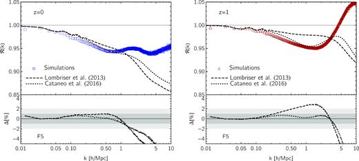
Matter power spectrum reactions in f(R) gravity for |$|\bar{f}_{R0}|=10^{-5}$|. In each panel the data points represent the reactions measured from simulations; lines denote the corresponding halo model predictions identified by the halo mass function used for the one-halo contributions in f(R) gravity, that is either Lombriser et al. (2013) (dashed) or Cataneo et al. (2016) fits (dotted). Lower panels present the fractional deviation of the halo model relative to the simulations, with grey bands marking the |$1\, {\rm per\, cent}$| and |$2\, {\rm per\, cent}$| uncertainty regions. Left: reaction at z = 0 with both halo mass functions providing predictions within |$1\, {\rm per\, cent}$| from the simulations for k ≲ 1 |$h \, {\rm Mpc}^{-1}$|, as shown in the lower panel. Right: z = 1 reaction. The lower panel shows that thanks to the improved semi-analytical prescription for the halo abundances in Cataneo et al. (2016) the agreement between halo model and simulations reaches per cent-level on scales k ≲ 1 |$h \, {\rm Mpc}^{-1}$|.
Given the complexity of measuring the virial halo mass function in f(R) simulations,12 we investigate changes in the reactions induced by a more accurate description of the halo abundances with the fits provided in Cataneo et al. (2016). There, however, the calibration of the |$n_\Delta ^{f(R)}/n_\Delta ^{\rm \Lambda CDM}$| ratios was performed for Δ = 300, whereas for our purposes we need Δ = Δvir. We go from one mass definition to the other with the scaling relations outlined in Hu & Kravtsov (2003) (for a first application to f(R) gravity see Schmidt et al. 2009). Inevitably, this transformation suffers from inaccuracies in cvir and Δvir, which we attempt to compensate for by adjusting the M300(Mvir) relation so that the new rescaled mass function provides a present-day halo model reaction that is at least as good as the reaction obtained when using the Lombriser et al. (2013) virial mass function (dotted line in the left-hand panel of Fig. 1).13 We then take the ratio of the Cataneo et al. (2016) rescaled mass function to that of Lombriser et al. (2013), and treat this quantity as a correction factor for the latter. To find the required adjustment at high redshifts we shift the z = 0 correction by an amount Δlog10Mvir inferred from the redshift evolution of the ratio of the two halo mass functions over the range z ∈ [0, 0.5] (see central panel of fig. 4 in Cataneo et al. 2016). A simple extrapolation to z = 1 gives Δlog10Mvir = 1. Although far from being a rigorous transformation, the resulting halo model reaction now agrees to better than 1 per cent down to k ≈ 3 |$h \, {\rm Mpc}^{-1}$|, as shown in the right-hand panel of Fig. 1. Fig. 2 illustrates that similar considerations are also valid for the F6 cosmology, where we use the same mass shift Δlog10Mvir = 1 to go from the z = 0 to the z = 1 mass function correction. In all cases, deviations in the highly non-linear regime are most likely caused by inaccurate c–M relations. We leave the study of f(R) gravity reactions on small scales derived from proper virial quantities for future work.

Figs 3 and 4 show the relative change of the matter power spectrum in f(R) gravity with respect to GR for the F5 and F6 models, respectively. The left-hand panels present the best-case scenario, that is, when ‘perfect’ knowledge of the pseudo power spectrum is available. In this case, since the uncertainties come entirely from our halo model predictions, we can obviously reproduce the power spectrum ratios at the same level of accuracy of our reactions. For now the pseudo information comes directly from our simulations, but it is not hard to imagine a specifically designed emulator capable of generating the non-linear matter power spectrum of ΛCDM cosmologies with non-standard initial conditions. We will analyse the requirements for such emulator in a future work (Giblin et al. in preparation). In the right-hand panels we compute Ppseudo with hmcode to demonstrate that currently, together with publicly available codes, our method can achieve 2 per cent accuracy on scales k ≲ 1 |$h \, {\rm Mpc}^{-1}$|in modified gravity theories characterized by scale-dependent linear growth.

Matter power spectrum fractional enhancements relative to GR for f(R) gravity with |$|\bar{f}_{R0}|=10^{-5}$|. As in the previous figures, the data points correspond to the results from simulations at z = 0 (blue squares) and z = 1 (red triangles). Coloured lines denote predictions based on the halo model reactions at z = 0 (dashed blue) and z = 1 (dot–dashed red). To emphasize the impact of non-linearities we include the linear theory predictions as dashed grey lines. Lower panels show the fractional deviation of the non-linear predictions from the simulations, |$\Delta \equiv \left(\mathcal {R} \times P_{\rm Pseudo}^{\rm Sim/HMcode}/P_{\rm GR}^{\rm Sim/HMcode} \right)/\left(P_{\rm Real}^{\rm Sim}/P_{\rm GR}^{\rm Sim} \right)-1$|, with grey bands marking |$1\, {\rm per\, cent}$| and |$2\, {\rm per\, cent}$| uncertainty regions. Left: for our theoretical estimates we use pseudo cosmology matter power spectra measured from simulations as the baseline, which we then rescale with the halo model reactions employing the Cataneo et al. (2016) halo mass functions. The lower panel illustrates that with future codes, eventually capable of reaching per cent-level accuracy on the matter power spectra for the ΛCDM-evolved pseudo cosmologies, high-accuracy non-linear matter power spectra in modified gravity will also be accessible. Right: same as left-hand panel with the difference that the pseudo cosmology matter power spectra computed with hmcode are now adopted as the baseline. This implies that applying our halo model reaction methodology to baseline ΛCDM predictions from existing codes we can achieve |${\lesssim}2\, {\rm per\, cent}$| precision on scales k ≲ 1 |$h \, {\rm Mpc}^{-1}$|.
Same as Fig. 3 with the background field amplitude set to |$|\bar{f}_{R0}|=10^{-6}$|.
For a comparison to a range of other methods for modelling the non-linear matter power spectrum in f(R) and other chameleon gravity models, we refer to fig. 4 and 5 in Lombriser (2014), noting that the majority of these methods rely on fitting parameters in contrast to the approach discussed here.
5.2 DGP
Spherical collapse dynamics is much simpler in nDGP (Schmidt et al. 2010), with both the linear overdensity threshold for collapse, δc, and the corresponding average virial halo overdensity, Δvir, being only functions of redshift. For instance, in GR one has Δvir(z = 0) = 335 and Δvir(z = 1) = 200 for Ωm = 0.3072, whereas these values become Δvir(z = 0) = 283 and Δvir(z = 1) = 178 in our nDGPm cosmology. This fact allows us to extract the virial halo mass function directly from our simulations, and test that accurate |$n_{\rm vir}^{\rm real}/n_{\rm vir}^{\rm pseudo}$| ratios do indeed produce accurate halo model reactions. Figs 5 and 6 show that, after refitting the virial ST mass function to the same quantity from simulations, halo model predictions reach per cent level accuracy on scales k ≲ 1 |$h \, {\rm Mpc}^{-1}$|(see Appendix C for details on the halo mass function calibration to simulations). Moreover, since the Vainshtein radius (equation 23) for the most massive haloes is of order a few megaparsecs, we expect small changes caused by the screening mechanism on large scales, i.e. k ≲ 0.1 |$h \, {\rm Mpc}^{-1}$|. In other words, although in our calculations we keep the two-halo correction factor in equation (53), it contributes only marginally to improving the performance of our reaction functions. This is evident from the perturbation theory predictions shown in Fig. B2. Once again, deviations on scales k ≳ 1 |$h \, {\rm Mpc}^{-1}$|could be primarily sourced by inaccurate real and pseudo halo concentrations, and is the subject of future investigation.

Matter power spectrum reactions in an nDGP cosmology with crossover scale rcH0 = 0.5. In each panel the data points represent the reactions measured from simulations; lines denote the corresponding halo model predictions defined by the halo mass function used for the one-halo contributions in nDGP gravity, that is based on either the standard ST fits (dashed) or on fits to our simulations presented in Appendix C (dotted). Lower panels present the fractional deviation of the halo model relative to the simulations, with grey bands marking the |$1\, {\rm per\, cent}$| and |$2\, {\rm per\, cent}$| uncertainty regions. Left: reaction at z = 0 with the refitted halo mass function significantly improving the predictions for k ≲ 1 |$h \, {\rm Mpc}^{-1}$|, as shown in the lower panel. Right: z = 1 reaction. The lower panel shows similar performance for the two halo mass function fits, with our refitted version matching the simulations within |$1\, {\rm per\, cent}$| over a wider range of scales.

We study the ability of the halo model reactions to reproduce the relative difference of the nDGP power spectrum from that of standard gravity when combined with the pseudo matter power spectrum from either hmcode or the simulations. Figs 7 and 8 confirm that with current codes also scale-independent modifications of gravity can be predicted within 2 per cent over the range of scales relevant for this work.

Matter power spectrum fractional enhancements relative to GR for nDGP with rcH0 = 0.5. The data points correspond to the results from simulations at z = 0 (blue squares) and z = 1 (red triangles). Coloured lines represent predictions based on the halo model responses at z = 0 (dashed blue) and z = 1 (dot–dashed red). To emphasize the impact of non-linearities we include the linear theory predictions as dashed grey lines. Lower panels show the fractional deviation of the non-linear predictions from the simulations, |$\Delta \equiv \left(\mathcal {R} \times P_{\rm Pseudo}^{\rm Sim/HMcode}/P_{\rm GR}^{\rm Sim/HMcode} \right)/\left(P_{\rm Real}^{\rm Sim}/P_{\rm GR}^{\rm Sim} \right)-1$|, with grey bands marking |$1\, {\rm per\, cent}$| and |$2\, {\rm per\, cent}$| uncertainty regions. Left: for our theoretical estimates we use pseudo cosmology matter power spectra measured from simulations as the baseline, which we then rescale with the halo model reactions employing our refitted halo mass functions in Appendix C. As for f(R) gravity, the lower panel illustrates that with future codes eventually capable of reaching per cent-level accuracy on the matter power spectra for the ΛCDM-evolved pseudo cosmologies, high-accuracy non-linear matter power spectra for scale-independent modifications of gravity will also be within reach. Right: same as the left-hand panel with the difference that the pseudo cosmology matter power spectra computed with hmcode are now adopted as the baseline. Current available codes can achieve |${\lesssim}2\, {\rm per\, cent}$| precision on scales k ≲ 1 |$h \, {\rm Mpc}^{-1}$|when used in combination with accurate halo model reactions.

Same as Fig. 7 with the crossover scale set to rcH0 = 2.
5.3 Dark energy
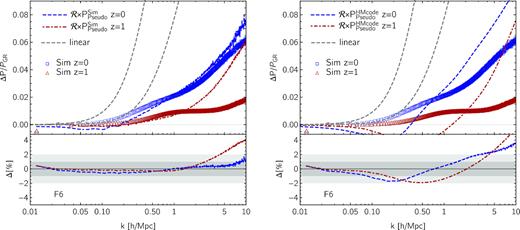
Fig. 9 shows the reaction functions for the evolving DE cosmologies listed in Table 1. The left-hand panel contains essentially the same z = 0 information of Fig. 2 in Mead (2017), with the notable difference that here we compute the spherical collapse virial overdensities including the DE contribution to the potential energy, and do not assume energy conservation during collapse (Schmidt et al. 2010) (expressions for the individual terms entering the virial theorem can be found in Appendix A). The right-hand panel shows the same quantity at z = 1. At both redshifts the halo model reactions based on the standard ST mass function fits can capture very well the measurements from simulations down to the transition scale between the two- and one-halo terms. Also in this case, we attribute inaccuracies on small scales mainly to the inadequacy of the Dolag et al. (2004) and Bullock et al. (2001) halo concentration prescriptions for the real and pseudo cosmologies, respectively.

Matter power spectrum reactions for the six DE cosmologies with {w0, wa} pairs listed in Table 1. In each panel, the data points represent the mean reactions measured from simulations as the average from three realizations; lines denote the corresponding halo model predictions. Lower panels show the fractional deviation of the halo model relative to the simulations, with grey bands marking the |$1\, {\rm per\, cent}$| and |$2\, {\rm per\, cent}$| uncertainty regions. Left: reactions at z = 0. These are similar to those presented in Mead (2017) and only differ in the derivation of the virial overdensity Δvir, in that here we account for all relevant contributions to the potential energy and do not assume energy conservation (see equations A6–A11). On small scales agreement with the simulations is somewhat better than in modified gravity, which can be ascribed to a more accurate c–M relation at z = 0. Right: z = 1 reactions. Although per cent level accuracy is reached on scales k ≲ 1 |$h \, {\rm Mpc}^{-1}$|, performance on highly non-linear scales deteriorates beyond the 2 per cent level for some models. We think part of the reason for that is to be found in high-z inaccuracies of the Dolag et al. (2004) prescription for the halo concentrations in DE cosmologies.
In Fig. 10 we consider two representative DE models, DE2 and DE3, and compare their matter power spectra to that of ΛCDM with the same initial conditions. Their particular equations of state enhance the growth of structure in one case and suppress it in the other. Here, we employ the Coyote Universe Emulator (Heitmann et al. 2014) not only for our baseline pseudo power spectra, but also as a substitute for the real and ΛCDM cosmology simulations. This serves as an example to illustrate a straightforward application of the reaction functions: extend the cosmological parameter space of matter power spectrum emulators designed for the concordance cosmology only, without the need to run model-dependent and expensive cosmological simulations. For the evolving equation of state of DE3 we use the emulator extension code PKequal built upon the work presented in Casarini et al. (2016). Knowing that the output from the emulator is 1–2 per cent accurate on scales k ≲ 1 |$h \, {\rm Mpc}^{-1}$|, from the previous results in Fig. 9 we can expect similar agreement between our reaction-based power spectra and those obtained from the emulator itself. This is indeed the case except in the range |$0.02 \lesssim k \, {\rm Mpc}\, h^{-1}\lesssim 0.5$|, where the interpolation process within the emulator fails to capture the correct dependence on ωb and w because the specific values we use sit on the edge of its domain of applicability.14

Matter power spectrum fractional differences relative to ΛCDM for DE3 (left) and DE2 (right) models, where the numbers in curly brackets specify the equation-of-state pair {w0, wa}. Data points correspond to the output from the Coyote Universe emulator (Heitmann et al. 2014) at z = 0 (blue squares) and z = 1 (red triangles). For DE3, which has a non-constant w, we used the emulator extension of Casarini et al. (2016). Coloured lines represent predictions based on the halo model reactions at z = 0 (dashed blue) and z = 1 (dot–dashed red). For reference, the linear theory predictions are shown as dashed grey lines. Lower panels show the fractional deviation of the non-linear predictions from the emulator, with grey bands marking |$1\, {\rm per\, cent}$| and |$2\, {\rm per\, cent}$| uncertainty regions. For our theoretical estimates we use pseudo cosmology matter power spectra computed with the emulator itself as baseline, which we then rescale with the halo model reactions. Lower panels illustrate that our halo model predictions can be employed to map accurately ΛCDM cosmologies to evolving DE models. Deviations of order |$2\!-\!4\, {\rm per\, cent}$| on scales |$0.02 \lesssim k \, {\rm Mpc}\, h^{-1}\lesssim 0.5$| are entirely due to the emulator being pushed to the edges of its domain of applicability in the plane {ωb, w}.
6 CONCLUSIONS
The spatial distribution of matter in the Universe and its evolution with time emerge from the interplay of gravitational and astrophysical processes, and are inextricably linked to the nature of the cosmic matter-energy constituents. The power spectrum is an essential statistic describing the clustering of matter in the Universe, and lies at the heart of probes of the growth of structure such as cosmic shear and galaxy clustering. Measurements of these quantities from the next generation of large-volume surveys are expected to reach per cent level uncertainty – upon careful control of systematics – on scales where non-linearities and baryonic physics become important. It is notoriously difficult to predict the matter power spectrum in this regime to such a degree of accuracy, yet these scales contain a wealth of information on currently unanswered questions, e.g. the nature of DE, the sum of neutrino masses, and the extent of baryonic feedback mechanisms.
In this work we focused on modelling the non-linear matter power spectrum in modified theories of gravity and evolving DE cosmologies. We extended the reaction method of Mead (2017) using the halo model to predict the non-linear effects induced by new physics on the matter power spectrum of specifically designed reference cosmologies. These fiducial – pseudo – cosmologies mimic the linear clustering of the target – real – cosmologies, yet their evolution is governed by standard gravity with ΛCDM expansion histories (which are either quick to simulate with current resources, if not already available with emulators). We showed that by applying the halo model reactions to the non-linear matter power spectrum of the pseudo cosmologies we are able to recover the real counterpart to within 1 per cent on scales k ≲ 1 |$h \, {\rm Mpc}^{-1}$|for all cases under study. Remarkably, our methodology does not involve fitting the power spectra measured in simulations at any stage. Instead, having access to accurate ratios of the halo mass function in the real cosmology to that in the pseudo cosmology is crucial to achieve the observed performance. Not including this information from the simulation degrades the accuracy to |${\lesssim} 3\, {\rm per\, cent}$|. The halo model reactions can also be used to predict the matter power spectrum in the highly non-linear regime. However, this requires additional knowledge of the average structural properties of the dark matter haloes as well as the inclusion of baryonic effects (see e.g. Schneider et al. 2019). We leave these improvements for future work (Cataneo et al. in preparation).
In the case of the DE models we adopted the Coyote Universe emulator for the pseudo matter power spectrum (i.e. for w = −1), which we then combined with our halo model reaction to obtain the real expected quantity. By comparing this prediction to the real output of the emulator (i.e. for w ≠ −1) we showed that emulators trained on pure ΛCDM models can be accurately extended to non-standard cosmologies in an analytical way, thus substantially increasing their flexibility while simultaneously reducing the computational cost for their design. However, applications of this strategy to scale-dependent modifications of gravity [such as f(R) models] necessitate of a more elaborate ΛCDM emulator that takes as input also information on the linearly modified shape of the matter power spectrum (Giblin et al. in preparation). Together with suitable halo model reactions, this emulator can also be employed to predict the non-linear total matter power spectrum in massive neutrino cosmologies (Cataneo et al. in preparation), where the presence of a free streaming scale induces a scale-dependent linear growth (Lesgourgues & Pastor 2006).
Given that our method builds on the halo model, the halo mass function and the spherical collapse model are absolutely central for our predictions. Contrary to the standard halo model calculations, however, the accuracy of our reactions strongly depends on the precision of the pseudo and real halo mass functions. This opens up the possibility of combining in a novel way cosmic shear and cluster abundance measurements, for example. Moreover, quite general modifications of gravity – with their screening mechanisms – can be implemented in the spherical collapse calculations through the non-linear parametrized post-Friedmannian formalism of Lombriser (2016).
In summary, halo model reactions provide a fast, accurate, and versatile method to compute the real-space non-linear matter power spectrum in non-standard cosmologies. Successful implementations in redshift-space by Mead (2017) pave the way for applications to redshift-space distortions data as well. Altogether, these features make the halo model reactions an attractive alternative in-between perturbative analytical methods and brute force emulation, and promise to be an essential tool in future combined-probe analyses in search of new physics beyond the standard paradigm.
ACKNOWLEDGEMENTS
We thank Philippe Brax, Patrick Valageas, Alejandro Aviles, and Jorge Cervantes-Cota for crosschecking our perturbation theory calculations, and David Rapetti and Simon Foreman for useful discussions. MC and CH acknowledge support from the European Research Council under grant number 647112. LL acknowledges support by a Swiss National Science Foundation (SNSF) Professorship grant (No. 170547), an SNSF Advanced Postdoc.Mobility Fellowship (No. 161058), the Science and Technology Facilities Council Consolidated Grant for Astronomy and Astrophysics at the University of Edinburgh, and the Affiliate programme of the Higgs Centre for Theoretical Physics. AM has received funding from the European Union‘s Horizon 2020 research and innovation programme under the Marie Skłodowska-Curie grant agreement No. 702971 and acknowledges MDM-2014-0369 of ICCUB (Unidad de Excelencia Maria de Maeztu). SB is supported by Harvard University through the ITC Fellowship. BL is supported by the European Research Council via grant ERC-StG-716532-PUNCA, and by UK STFC Consolidated Grants ST/P000541/1 and ST/L00075X/1. This work used the DiRAC Data Centric system at Durham University, operated by the Institute for Computational Cosmology on behalf of the STFC DiRAC HPC Facility (www.dirac.ac.uk). This equipment was funded by BIS National E-infrastructure capital grant ST/K00042X/1, STFC capital grants ST/H008519/1, ST/K00087X/1, STFC DiRAC Operations grant ST/K003267/1 and Durham University. DiRAC is part of the National E-Infrastructure.
Footnotes
Here and throughout we work in natural units, and set c = 1.
See, however, the recent work by He et al. (2018) where it was showed that deviations as small as |$|\bar{f}_{R0}| =10^{-6}$| could already be in strong tension with redshift space distortions data. At this time, the tightest constraints on f(R) gravity come from the analysis of kinematic data for the gaseous and stellar components in nearby galaxies, which only allows |$|\bar{f}_{R0}| \lesssim 10^{-8}$| (Desmond et al. 2018).
This is an assumption made to ease comparisons to ΛCDM simulations, and is not a strict observational requirement (cf. Lombriser et al. 2009).
For cosmologies with a scale-independent linear growth, such as nDGP and wCDM, using the ΛCDM growth is simply a matter of convenience. In f(R) gravity this approach has the advantage of preserving the statistics of the initial mass fluctuations. For more details see Cataneo et al. (2016).
In this instance, and whenever the context is clear, we omit the time-dependence from our notation. However, we reintroduce it any time this can become a source of ambiguity.
Valogiannis & Bean (2019) recently found that in f(R) gravity the linear halo bias contains an additional term accounting for the environmental dependence, which we omit in equation (43). Given the relative unimportance of the bias for our halo model reactions (see Sections 3.3 and 5), this choice is, in effect, inconsequential for the accuracy of our predictions.
Note that in Mead (2017) this is referred to as response. We use the term reaction to distinguish it from the quantities studied in Neyrinck & Yang (2013), Nishimichi, Bernardeau & Taruya (2016), or Barreira & Schmidt (2017). Our and these other definitions are all conceptually analogous, in the sense that they describe how the non-linear power spectrum responds to changes in some feature, which in our case is physics beyond the vanilla ΛCDM cosmology, e.g. fifth forces, evolving DE, massive neutrinos, baryons etc.
Note that we neglect the integral factor equation (50) in our two-halo terms. We checked that setting I2(k) = 1 for all scales has no measurable impact on our halo model reactions.
This is not strictly true in the traditional halo model implementation we adopt in this work. In fact, the one-halo terms have a constant tail in the low-k limit (see equation 54) that dominates the two-halo contributions on very large scales. In a consistent formulation of the halo model, however, where mass and momentum conservation are enforced, this tail disappears leaving only the theoretically motivated two-halo term (Schmidt 2016). For our purposes we can simply ignore this inconsistency, and restrict the use of the reaction function to scales k > 0.01 |$h \, {\rm Mpc}^{-1}$|.
As we shall see below, k⋆ is derived from perturbation theory and is largely independent of the one-halo contribution. However, its specific value should be interpreted with caution, in that equally good alternatives to the exponential function in equation (53) can provide different solutions to equation (55).
Due to the nature of the chameleon screening, in f(R) gravity the virial overdensity depends on both the mass of the halo and the gravitational potential in its environment. Things are much simpler in DGP, where by virtue of the Vainshtein screening both dependencies disappear.
In practice, we start with the Hu & Kravtsov (2003) relation |$M_{300} = \mathcal {Q}(M_{\rm vir})M_{\rm vir}$|, and make the replacement |$\mathcal {Q}(M_{\rm vir}) \rightarrow \mathcal {Q}^{\prime }(M_{\rm vir}) = \min [{\tilde{a}}\mathcal {Q}^{f(R)}({\tilde{b}}M_{\rm vir}),\mathcal {Q}^{\rm GR}(M_{\rm vir})]$|, where |${\tilde{a}}$| and |${\tilde{b}}$| are |$\mathcal {O}(1)$| free parameters fine-tuned to reach the required accuracy in the halo model reaction at z = 0. The use of the minimum operator ensures that the f(R) conversion factor matches the corresponding GR value for masses large enough to fully activate the chameleon screening.
The Coyote Universe emulator accepts values 0.0215 < ωb < 0.0235 and −1.3 < w < −0.7, while for our two evolving DE models we have ωb = 0.0245, w(DE2) = −1.3, and |$w_{\rm eff}^{\rm (DE3)} = -0.84$|. Since our background baryon density resides outside the domain of the emulator, we set it to the maximum value allowed. This has virtually no impact on our halo model responses, in that they depend only weakly on ωb.
REFERENCES
APPENDIX A: SPHERICAL COLLAPSE IN MODIFIED GRAVITY AND QUINTESSENCE
We shall briefly review expressions for the force enhancement |$\mathcal {F}$| in f(R) and DGP gravity used in the modified spherical collapse calculation in Section 3.1 as well as its impact and the impact of DE domination on the virial theorem.
APPENDIX B: PERTURBATION THEORY
The non-linear evolution of matter perturbations in modified gravity has been extensively studied in Koyama et al. (2009), Brax & Valageas (2012), Brax & Valageas (2013), and Bose & Koyama (2016). Here we summarize their results and provide explicit expressions for the computation of next-to-leading-order corrections to the linear power spectrum.
To deactivate the screening mechanisms we simply set γ2; 11 = σ2; 111 = 0, while keeping the linear deviation ϵ given in equations (B6)–(B7). This results in what we call the real ‘no-screening’ power spectrum, |$P_{\rm NoScr}^{\rm real}$|. The pseudo power spectrum up to one-loop, instead, follows from also imposing ϵ = 0, such that the only difference compared to the standard cosmology is in the initial conditions, i.e. in the shape and/or amplitude of the linear power spectrum. Figs B1 and B2 show the SPT reaction functions on quasi-linear scales for f(R) gravity and nDGP, where the pseudo non-linear power spectrum is computed using either the pseudo (solid lines) or ‘no-screening’ (dashed lines) one-loop correction. Although the former approach is theoretically motivated, accuracy arguments make the latter preferable for all cosmologies and redshifts investigated in this work.

SPT matter power spectrum reactions in f(R) gravity with background scalaron amplitudes |$|\bar{f}_{R0}|=10^{-5}$| (left) and |$|\bar{f}_{R0}|=10^{-6}$| (right). The different lines illustrate the effect of computing the non-linear power spectrum for the pseudo cosmology using either the exact one-loop corrections (solid) or the real unscreened one-loop terms instead (dashed). The squares are the measurements from our simulations. In F5 the real screened and unscreened one-loop contributions err in the same direction, which makes the no-chameleon correction preferable over the theoretically motivated pseudo one-loop term. The opposite is true for F6, although the difference between the two approaches is small in this case. For consistency, throughout this work we always choose the ‘no-screening’ one-loop correction for our pseudo SPT predictions, a strategy good enough on large quasi-linear scales for all cosmologies investigated.

Same as Fig. B1 for nDGP gravity with crossover scales rcH0 = 0.5 (left) and rcH0 = 2 (right). Here using the real unscreened one-loop corrections instead of the equivalent exact pseudo quantity has negligible impact on the SPT responses.
APPENDIX C: HALO MASS FUNCTION AND CONCENTRATION TESTS
In Section 3.3 we showed that the real to pseudo halo mass function ratio, |$n_{\rm vir}^{\rm real}/n_{\rm vir}^{\rm pseudo}$|, controls the halo model reaction on scales k ≳ 0.1 |$h \, {\rm Mpc}^{-1}$|. In particular, for the nDGP cosmologies we explicitly checked that fitting the semi-analytical halo mass functions directly to our simulations results in better performance of the halo model reactions for wavenumbers |$0.1 \lesssim k \, {\rm Mpc}\, h^{-1}\lesssim 1$|. Below we briefly explain how these fits to the halo mass functions extracted from our simulations were carried out.
We measure the mean halo abundances and their uncertainties from simulations as outlined in Cataneo et al. (2016), with the important difference that, here, haloes identified with the rockstar halo finder (Behroozi, Wechsler & Wu 2013) have masses defined in spherical volumes with mean density Δvir times the background comoving matter density, as in equation (36). The virial overdensity depends on redshift, matter content, and theory of gravity through equation (37). Compared to Cataneo et al. (2016) we also use a finer mass binning, with a bin size Δlog10M = 0.1. Figs C1 and C2 present a rescaled version of the halo mass functions (i.e. the large-scale limit of the one-halo integrand equation (49)) as well as the |$n_{\rm vir}^{\rm real}/n_{\rm vir}^{\rm pseudo}$| ratios. The standard halo mass function fits for the parameters in equation (41) systematically underpredict the simulation measurements. Refitting these parameters to each real and pseudo simulation separately can change the halo mass function ratio |$n_{\rm vir}^{\rm real}/n_{\rm vir}^{\rm pseudo}$| to an extent relevant for the halo model reactions. Note that when this ratio remains largely unaffected by the refitting, the predicted reactions also show very little variation (compare the right-hand panels of Figs C2 and 6). Table C1 summarizes the refitted ST halo mass function parameters for the real and pseudo nDGP cosmologies used in this work.

|$P_{1\rm h}(k \rightarrow 0)$| integrands (equation 49) at z = 0 (left) and z = 1 (right) for the nDGP cosmology with crossover scale rcH0 = 0.5. The data points with error bars are Jackknife estimates from simulations; lines correspond to semi-analytical predictions using the standard ST halo mass function fits {A, q, p} = {0.3222, 0.75, 0.3} (dashed), or to direct fits to our simulations (solid). Top panels show the results for the real nDGP cosmology, while middle panels present the outcome for the pseudo counterpart. The ratios of the real halo mass functions to the pseudo ones are illustrated in the lower panels. Combined with the information in Fig. 5, these ratios clearly stand out as the relevant quantity to achieve per cent level accuracy for the reaction function over scales k ≲ 1 |$h \, {\rm Mpc}^{-1}$|. In fact, the difference between the standard and refitted halo mass functions is more significant at low redshift, which reflects the performance shown in the lower panels of Fig. 5.

| Model | A | q |
|---|---|---|
| nDGPm (z = 0) | 0.3427 | 0.819 |
| nDGPm (z = 1) | 0.3067 | 0.757 |
| nDGPw (z = 0) | 0.3347 | 0.819 |
| nDGPw (z = 1) | 0.3023 | 0.754 |
| pseudo-nDGPm (z = 0) | 0.3438 | 0.829 |
| pseudo-nDGPm (z = 1) | 0.3057 | 0.761 |
| pseudo-nDGPw (z = 0) | 0.3332 | 0.823 |
| pseudo-nDGPw (z = 1) | 0.3013 | 0.753 |
Given the structure of the one-halo term equation (49), one might argue that inaccurate halo profiles are partially responsible for the few per cent mismatch between the predicted and measured reactions in Figs 1 and 5. If that was the case, then having accurate halo mass functions would not necessarily correspond to having accurate halo model reactions. However, Fig. C3 shows otherwise, in that even extreme variations of the halo concentrations cause important changes only on scales k ≳ 0.5 |$h \, {\rm Mpc}^{-1}$|.

Impact of the c–M relation on the nDGPm halo model response at z = 0. Lines correspond to different combinations of normalization and slope in equation (46), and changes are restricted to the real cosmology only. Even significant deviations from the standard values (solid blue line) are not able to match the simulations, with virtually no effect on scales k ≲ 0.5 |$h \, {\rm Mpc}^{-1}$|.
From these tests we conclude that accurate virial halo mass function ratios are central to determining |${\lesssim}1\, {\rm per\, cent}$| accuracy for the halo model reactions, and that the mean concentration of massive haloes is well described by equation (46), at least as long as this relation is employed in the reaction ratios. In future works we will investigate the implications of refitting the c–M relation to that measured in simulations, which has the potential to ameliorate our halo model predictions in the highly non-linear regime.
