On the detectability of transiting planets orbiting white dwarfs using LSST Free

ABSTRACT

1 INTRODUCTION

The vast majority of stars end their lives as white dwarfs (WDs). Within these stellar remnants, nuclear fusion has ceased and thus further inward collapse is resisted by electron degeneracy pressure. As a result, these remnants have compact radii similar to that of the Earth, yet with a mass of typically half of that of the Sun. Despite the absence of internal fusion, these stars shine for billions of years as they slowly cool, providing a means of studying their behaviour and environment.

In recent years, there has been increasing interest in searching for and studying planets orbiting ever smaller primaries (Reich 2013). In the early years of the modern exoplanet era, surveys typically focused on FGK stars resembling the Sun (e.g. Bakos et al. 2004; Pollacco et al. 2006; Wilson et al. 2008; Bakos et al. 2013). A basic argument was that such stars clearly have a credible chance of supporting life as demonstrated by our own existence, but smaller primaries (in particular M-dwarfs) may be less favourable¹ (e.g. see Dole 1964; Kasting, Whitmire & Reynolds 1993). Both radial velocity surveys, such as HARPS (Bonfils et al. 2013), and photometric surveys, such as MEarth (Charbonneau et al. 2009; Irwin et al. 2015), began to shift the focus towards smaller M-dwarfs, arguing that their smaller dimensions provide a significant boost to sensitivity. The discovery by Kepler that early-type M-dwarfs appear to host more planets, including habitable-zone planets, than Sun-like stars (Dressing & Charbonneau 2015) has brought M-dwarfs keenly into focus of planet hunters in recent years.

Surveys such as SPECULOOS (Burdanov et al. 2017) aim to push down further to late-type M-dwarfs as suitable targets for hunting planets. Surveys for planets orbiting even smaller and fainter brown dwarfs appear imminent (Triaud et al. 2013). Clearly then, the field of exoplanets has departed from the paradigm that we should only survey types of stars where we know for certain life is possible. There are certainly many challenges to life as we know it surviving and thriving on planets such as Proxima b (Anglada-Escudé et al. 2016) with a rich and active debate taking place in the literature (Ribas et al. 2016; Turbet et al. 2016; Garcia-Sage et al. 2017). Against this backdrop, an open-minded philosophy for allocating observational resources and effort is to focus on looking for life in places where we have the ability to observationally test it, not necessarily the places which we hypothesize as being the most habitable.

It could be argued that the pinnacle of this drive towards ever smaller planet hosts is represented by white dwarfs.² With a radius of about 10 times less than that of the smallest M-dwarf (Shipman 1979; Chen & Kipping 2017), these stars provide a major amplification of transit signals of up to 100-fold. On the downside, these stars are intrinsically faint, meaning that they are quite uncommon in a magnitude-limited survey. Further, their small dimensions mean that transits would last for minutes, not hours, posing a challenge to conventional surveys whose integration times are often too long to resolve the signals (Jenkins et al. 2010a).

The potential value of a WD exoplanet survey was highlighted by Faedi (2011) and Agol (2011), who argued that at least a few thousand WDs need to be surveyed to place meaningful constraints on their existence. The largest survey of WDs for transiting planets to date was recently published by Van Sluijs & Van Eylen (2018), who found no examples amongst |$1148$| WDs observed by K2. If such planets could be found, Loeb & Maoz (2013) estimate that only a few hours of JWST time would be needed to analyse their atmospheres (should they exist) thanks to the small size of the host.

At first, it may seem a stretch to consider WDs as potential planet hosts. These stars would have been red giant stars at some point, engulfing any planets within an au (Sandquist et al. 1998, 2002). Despite this, there are now numerous indirect clues suggesting planets may indeed orbit WDs. First, ∼30 per cent of WDs appear to have metal contaminated atmospheres, indicative of a continuous supply of in-falling rocky material as a result of short diffusion time-scales (Zuckerman et al. 2003, 2010; Koester, Gänsicke & Farihi 2014). Secondly, debris discs appear common around WDs, potentially supporting a second generation of planet formation. Active research places lower limits between 1 per cent and 5 per cent (Barber et al. 2012; Debes, Walsh & Stark 2012). Thirdly, there is direct evidence of a likely disintegrating body orbiting WD 1145+017 (Vanderburg et al. 2015). Put together, these clues strongly motivate that we should at least attempt a deep search for planets orbiting white dwarfs.

As alluded to earlier though, there are two significant obstacles facing any survey attempting to seek WD planets. First, WDs are faint and thus in order to survey a large number we need to survey both a large fraction of the sky and go deep (Kilic et al. 2013). Secondly, the transits last for minutes, meaning that exposures must not exceed that time-scale in order to avoid significant distortion and dilution of the transit morphology (Kipping 2010). LSST is essentially completely unique in being able to overcome these two challenges. The sample size issue will be certainly overcome, since LSST will observe down to m_r ≈ 24, including an expected ∼10⁷ WDs (Agol 2011). The problem of transit distortion is also overcome since LSST is expected to take two 15 s exposures back to back in normal operation, sufficient to avoid smearing of the light curve (Abell et al. 2009). Additionally, even if LSST switches to a single 30 s exposure, issues should not be encountered as long as long-term stability for the planetary systems being observed has been achieved.

The most obvious drawback in using LSST for this purpose is that it does not survey each patch of the sky for long periods of time. Thus, ignoring the deep drilling fields, one should never reasonably expect a particular instance of WD transit to be covered, only a partial transit. However, if the signal is strictly periodic, then it is not the temporal coverage which we actually care about but rather the phase coverage (Lund et al. 2015). Over the 10 yr baseline of LSST we should expect well-suited phase coverage for any given star.³

For the reasons described above, we hypothesized that LSST would be an excellent machine for searching for WD transiting planets. However, a detailed study injecting real transit signals into LSST-like sparsely sampled time series around realistic WDs is notably absent in the literature and thus reasonable concerns might exist about the true feasibility of detecting WD planets with LSST. In response to this, the work presented in what follows offers a detailed suite of simulations of planets injected into LSST light curves to evaluate their detectability.

In Section 2, we describe our method for generating a WD catalogue and simulating light curves from an LSST sample cadence. In Section 3, we explain our approach for injecting planet signals into the WD light curves, define sensitivity and detectability, describe our method for recovering planet signals, and explore a WD’s temperate zone. Finally, in Section 4, we discuss the implications of this work.

2 SIMULATING LSST LIGHT CURVES

2.1 Overview: a Monte Carlo approach

The primary objective of this work is to evaluate the detectability of transiting planets with LSST. An unconditional yield estimate is not formally calculable in the absence of any information about the occurrence rate and distribution of planets orbiting WDs. Instead, we aim to ask the question, if a WD hosted a planet with radius R_P and orbital period P, how detectable would that planet be using LSST?

This question is tackled from a Monte Carlo perspective using numerical simulations. While it may certainly be possible to express a reasonable parametric model describing the detectability of WD planets using analytic arguments, it is clearly complicated by the sparse non-uniform scheduling expected with LSST (Abell et al. 2009). A Monte Carlo approach is attractive if there exists a means of generating representative photometric time series expected from LSST for WDs. Unpacking that statement, the requirements of such an approach can be more specifically stated as being (a) the need to simulate a representative distribution of the properties of WDs that will be observed by LSST (b) the need to simulate representative photometric time series expected of said stars, accounting for realistic LSST noise and scheduling constraints.

Fortunately, both of these requirements are satisfied by software resources made available by the LSST team, namely opsim (Coffey, Saha & Miller 2006) and catsim. Using these tools, we describe in what follows how we generate representative photometric time series of WDs that will be observed by LSST. We discuss our approach for measuring planet detectability later in Section 3.

2.2 Generating a WD catalogue with catsim

LSST’s Catalog Simulator (catsim) is used to incorporate a realistic distribution of WDs within the Milky Way Galaxy. WDs, and all stars accessed by catsim are generated by galfast, a GPU-accelerated package that fits models of a thick and thin disc, and halo to SDSS data (Juric et al. 2008). The default simulated universe accessed by the catsim stack is stored as a database (Connolly et al. 2010, 2014) on a machine located at the University of Washington. Information for all WD’s with |$T_{\mathrm{eff}}\le 11\, 000$| K was retrieved and stored locally. The temperature constraint is imposed for the following reasons: (1) WDs with |$T_{\mathrm{eff}}\gt 11\, 000$| K will have |$L \gt 10^3\, \mathrm{ L}_\odot$| and will thus cool to |$T_{\mathrm{eff}}\lt 11\, 000$| K within a Gyr (Althaus et al. 2010) and (2) WDs, such as DAVs and DBVs, can exhibit pulsations above |$11\, 000$| K (Winget et al. 1982; Bergeron et al. 2004).

2.3 Interpolating stellar properties

Stars listed in the database accessed by catsim state the log g and T_eff of each source. However, in order to inject a planet around a given WD, we need to know the stellar mass, M_⋆, allowing us to convert a chosen orbital period into semimajor axis via Kepler’s Third Law. Rather than simply adopt a uniform stellar density for all WDs, we seek to create the most realistic catalogue possible in this work. Accordingly, we elected to estimate a realistic stellar mass for each WD based on the provided catsim information.

To accomplish this, we used the evolutionary cooling models of hydrogen- and helium-atmosphere white dwarfs⁴ from Holberg & Bergeron (2006), Kowalski & Saumon (2015), Tremblay, Bergeron & Gianninas (2011), and Bergeron et al. (2011). We perform a bi-linear interpolation of these model grids such that for any combination of log g and T_eff, we are able to assign a unique stellar mass. We find that both the DA and DB WD masses approximately follow a normal distribution peaked at half a solar mass with a ∼0.1 M_⊙ standard deviation.

2.4 Generating light curves with opsim and catsim

To generate mock observations, LSST’s Operations Simulator (opsim) is used in conjunction with catsim.⁵ A sample cadence for LSST’s 10 yr observing strategy is provided by opsim; we make use of the minion_1016 reference run. As currently configured, the catsim stack will only produce light curves for objects that incorporate a variability model; thus, we set the variability constraint within LightCurveGenerator.py of catsim to ‘None’. At this point, we are able to retrieve light-curve data (time, magnitude, errors) for all WDs.

To avoid memory issues on our local machine, we excluded data for WDs within ±25^○ of Galactic longitude, as seen in Fig. 1. Additionally, this constraint has the added benefit of exploring regions which are less affected by crowding.⁶ All WD light curves were stored locally on a database file.

Figure 1.

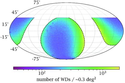
Number density of catsim generated WDs used in our survey. The Galactic plane is masked to within 25^○ in this work.

Open in new tabDownload slide

We briefly point out that the light curves generated assume that the visit-to-visit calibration error is much less than that of the point-to-point photometric uncertainty. Given our sources are generally faint, the point-to-point uncertainties are already large meaning that if LSST achieves visit-to-visit calibrations of the order of a per cent or better, this is unlikely to be a meaningful source of error⁷.

3 PLANET INJECTION AND RECOVERY

3.1 Overview

In order to calculate the detectability of planets around WDs with LSST, it is of course necessary to inject planets into our synthetic light curves described in Section 2, and so we turn our attention to this here.

As touched on earlier, the distribution and occurrence rate of planets around WDs is broadly unknown, making yield estimates, at best, conditional. Accordingly, we place our emphasis here on estimating the marginalized detectability of a planet of a given size and period. The process of marginalization is discussed in Section 3.4.

3.2 Injecting planets

Using a random subset of 3.5 million of our 10⁷ simulated WD light curves, we inject a single planet around every star with a random orbital period and physical radius. Periods are drawn from a log-uniform distribution between 0.15 and 10 d, and radii from a log-uniform distribution from |$\tfrac{1}{16}$| R_⊕ to 16 R_⊕. A random impact parameter, b, between 0 and 1 + (R_P/R_⋆) is assigned to each planet, such that a transit is guaranteed. The time of inferior conjunction, ϕ, is randomly assigned for each, and every planet is assumed to follow a strictly circular Keplerian orbit. We note that we do not consider eccentricity in this study. Given that the periods considered here are so short that the Roche limit already carves away a portion of the parameter space, as evident in Section 3.4, and that eccentricity primarily affects transit probability rather than light-curve shape (Kipping & Sandford 2016), we conclude eccentricity will not significantly affect our results.

Light curves for the injected planets are simulated using batman (Kreidberg 2015) assuming a 15 s integration time and uniform limb darkening. In all cases, we assume that the eventual 10 yr time series is available for the analysis. Further, we also highlight that we assume only a single planet for each star and that 100 per cent of the stars have planets. It is straightforward to scale our results for arbitrary occurrence rates later.

For each star, we calculate the planet’s signal-to-noise ratio (S/N) and assign a yes/no binary flag as to whether LSST is deemed to be sensitive to said planet (using the method described in Section 3.3). Accordingly, amongst the 3.5 million stars, we can select those that have planets within a local size- and period-bandwidth of a particular choice of R_P and P, and then simply count up what fraction of the stars had planets that LSST was sensitive to. This would therefore represent the marginalized sensitivity. This exercise could be repeated but instead using only a subset of the 3.5 million stars – for example taking just the bright end. In this way, the marginalized sensitivity can be computed using whatever marginalized sample one desires.

3.3 S/N and sensitivity

In this work, we inject planets but we do not blindly recover them. The sensitivity of LSST to a given planet is computed by evaluating the S/N instead. This choice was largely motivated by computational practicality. Running a box least-squares blind search (Kovács et al. 2002) on 3.5 million light curves would represent a major computational challenge.

In order to assess whether LSST is deemed to be sensitive or non-sensitive to a particular planet, we use a simple S/N threshold. Therefore, signals with a S/N exceeding the threshold are always defined as LSST-sensitive, and otherwise insensitive. This is a simplifying assumption since real transit surveys do not have step functions sensitivity curves at a particular threshold but rather S-like curves centred around a certain value (e.g. see Christiansen et al. 2016). Nevertheless, certainly recoverability does saturate to unity beyond a certain point and thus a threshold is not an unreasonable approximation. Ultimately, the true curve will not be known until real data becomes available. We adopt an S/N threshold of 7.1 in what follows, as this was the same value initially adopted by the Kepler team (Jenkins et al. 2010b) and thus provides a standardized point of comparison.

In practice, the S/N is computed using all of the available LSST bandpasses in conjunction to maximize our sensitivity to transit signals. An example of this is shown in Fig. 2 for illustration.

Figure 2.

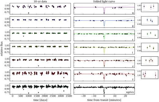
Sample light curves demonstrating 10 yr simulated observations (left) and phase folded data (right) across all six LSST filters (ugrizy); injected planet light curve included for reference. Injected planet properties: R_P/R_⋆ ≈ 0.60, |$P\approx {4.4\,\rm \mathrm{ h}}$|⁠, b ≈ 0.63, ϕ ≈ 1.4π.

Open in new tabDownload slide

3.4 Sensitivity in period–radius plane

The sensitivity of LSST to each system is clearly quite varied and depends on the star’s magnitude, position, observing cadence, etc. To simplify the picture, we calculate a so-called marginalized sensitivity as a function of R_P and P.

This is accomplished by first defining a local size- and period-bandwidth and then moving across a two-dimensional grid of R_P and P and calculating the local sensitivity as the number of positives in that window divided by the total stars in that window. In this way, the estimate has marginalized (or averaged) over all other parameters, such as stellar properties.

We define a bandwidth such that our periods and radii are divided into 40 evenly spaced grid points in logarithmic space, which we found provides a good balance of sufficient numbers per bin as well sufficient number of bins. The resulting marginalized sensitivities are plotted in Fig. 3 and are made publicly available at https://github.com/jicortes/whiteworlds. In our grid, it is apparent that we have removed some of the shortest period objects from our sample. These censored objects fall within the Roche limit of the star, where we have converted planetary radii into masses and then densities using the forecaster empirical mass–radius relation (Chen & Kipping 2017).

Figure 3.

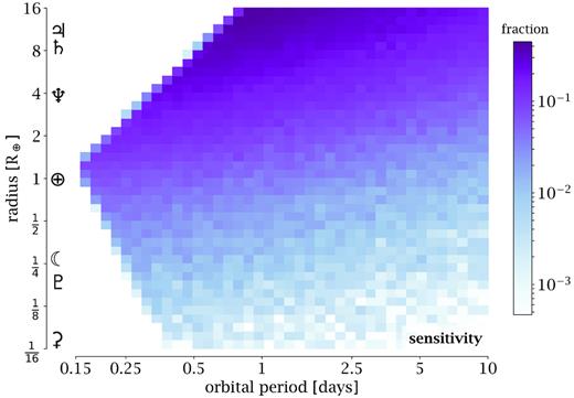
Sensitivity results plotted as a function of period and radius from our LSST simulations.

Open in new tabDownload slide

It is important to remember that sensitivity does not account for transit probability and thus one might reasonably expect sensitivities approaching unity for optimal cases. Indeed, the dynamic range apparent in Fig. 3 reflects this. As expected, short-period planets are evidently more easily detected than their longer period brethren due to the increased frequency of their transits. The strongest bias occurs along the radius axis, where naturally larger planets are much more easily detected.

where k is a free parameter quantifying the steepness of the logistic curve and log P₀ is a free parameter defining the mid-point.

where we find the values a = 18.77, b = 0.393, and c = −0.943 provide an excellent fit. The positive value for b indicates that longer period planets are more difficult to detect, close to a P^−2/5 dependence. The reason why the scaling is better than P^−1/2, which one would expect if considering purely the transit frequency scaling, is due to the effect of increased durations at longer P being preferentially detectable.

The negative c coefficient indicates a roughly linear scaling of sensitivity with respect to planet size. The relationship is not quadratic, as one might naively expect, due to the fact that most of the detectable region of our parameter space occurs for R_P > R_⋆, where quadratic scaling is not expected due to the total-eclipse and grazing-nature of the transits which dominate.

We highlight that directly comparing these coefficients to the theoretical expectations (e.g. from Kipping & Sandford 2016) is not generally possible since conventional transit yield/bias calculations do not operate in a regime dominated by grazing configurations. Nevertheless, equation (3) with the quoted coefficients provides a straightforward way for the community to use our sensitivity results in other studies.

3.5 From sensitivity to detectability

So far, our discussion has focused on sensitivity, which is defined under the assumption that the impact parameter, b, is uniformly distributed between zero and 1 + R_P/R_⋆. Thus, all stars are assumed to have a transiting planet. Of course, even if all of the stars have planets, they will not all host transiting planets. We therefore define marginalized detectability as being similar to marginalized sensitivity except we now account for the geometric transit probability expected for each planet.

To compute detectability, we multiply the yes/no binary flags (1: yes, 0: no) by the geometric probability of Pr(0 < b < 1 + R_P/R_⋆), which equals (R_⋆ + R_P)/a. Once each planet has a detection probability assigned, we draw a random Bernoulli integer to define the injected planet as being detected or non-detected. We are then able to compute a marginalized detectability in a similar fashion to that described earlier for sensitivity.

3.6 Detectability in period–radius plane

Our detectability results, accounting now for transit probability, are illustrated in Fig. 4 and are also made available at https://github.com/jicortes/whiteworlds. Broadly speaking, the pattern appears similar to that of sensitivity, except the resulting scores are typically two orders of magnitude lower, reflecting the ∼1 per cent transit probability of our injected planets. The dynamic range increases due to longer period planets being particularly unlikely to transit.

Figure 4.

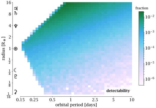
Detectability, which accounts for the geometric transit probabilities, plotted as a function of period and radius from our LSST simulations.

Open in new tabDownload slide

The mean detectability across all simulations equals 0.107 per cent, implying that roughly 1 in |$1000$| WD systems harbouring planets need to be surveyed by LSST to obtain a single detection. We find that, marginalized across radius, the mean detectability drops off as ∼1/P, peaking at 1.5 per cent for the shortest Roche-stable period possible (P = 4 h) and dropping down to 0.025 per cent at P = 10 d.

Using these numbers, it is straightforward to estimate yields for various occurrence rates. If 100 per cent of the ∼10⁷ WD stars observed by LSST harbour a planet with P < 10 d (i.e. η = 1) then we would expect |$10\, 700$| detections. Thus, we would require η ≲ 10⁻⁴ in order for LSST to detect no examples of transiting WD planets. On this basis, an LSST survey for WD transiting planets would be highly informative, either delivering many examples of a new class of planetary system or demonstrating to high confidence such systems are rare.

Although the log-uniform distributions in period and radius are likely as good as a choice as any other, the more arbitrary choice in our prior is the minimum/maximum period/radius. Changing these bounds will strongly influence a marginalized yield estimate, such as that made above. Rather than go through various hypothetical and speculative scenarios for these bounds, we prefer to focus on the more robust kernel density estimates for detectability (i.e. those shown in Fig. 4), which highlight that amongst a sample of 10⁷ WDs, the vast majority of parameter space should be expected to yield detections.

3.7 Detection bias

Armed with our numerical simulations, it is possible to investigate the impact of detection bias on our results. White dwarfs were generated as a representative astrophysical population using catsim, but planet detections will clearly favour brighter stars and bigger planets. Fig. 5 compares the detected versus injected population for four key parameters. We find that the stellar masses and radii of detected cases are representative of the true population. However, the detected stars tend to be hotter and thus more luminous making their photometric time series better quality for planet detections. The strong and expected bias towards larger planets is also recovered.

Figure 5.

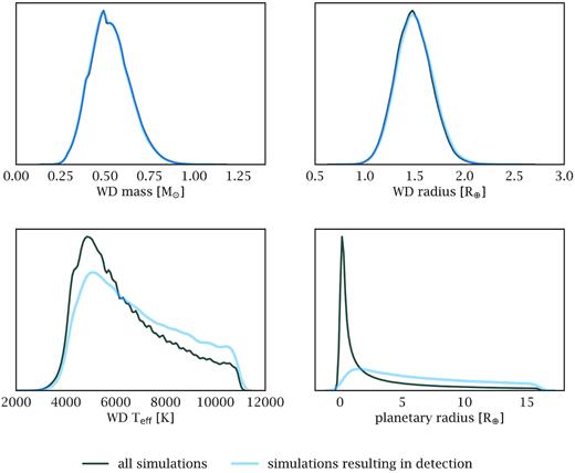
Comparison of the system properties between the injected and detected populations.

Open in new tabDownload slide

3.8 Detectability of temperate transiting WD planets

A strong motivation behind the search for planets outside of our Solar system is the potential characterization of habitable worlds, we thus turn our attention to a WD’s temperate zone here. As discussed in Agol (2011), given a WD’s mass and type (either H-rich or He-rich), a planet requires a specific orbital distance to fall within the continuously habitable zone (CHZ). This is defined as the range of orbital radii for which a planet will receive the necessary flux to sustain liquid water on its surface for at least 3 Gyr. We take the outer limits of the CHZ for an H-rich and He-rich WD from Agol (2011) and reassess the detectability results shown in Fig. 4. We note that the inner limit of the CHZ comes up against the tidal disruption limit and thus can essentially be ignored in what follows.

We re-cast our detection figure in terms of WD mass and semimajor axis, so we can directly draw the CHZ contours from Agol (2011) on top. In this way, the x-axis is essentially re-scaled via Kepler’s Third Law from the version in Fig. 4. The y-axis has replaced planetary radius with stellar mass, which was previously a marginalized quantity. It is therefore clear that in the revised version here, planetary radius will be a marginalized quantity. Specifically, we marginalize planets in the range 0.5 ≤ (R_P/R_⊕) ≤ 1.5 to focus on the potentially terrestrial-like planets. Finally, we split our sample into H-rich and He-rich stars, since the CHZ is noticeably different between the two (Agol 2011). The final results are shown in Fig. 6.

Figure 6.

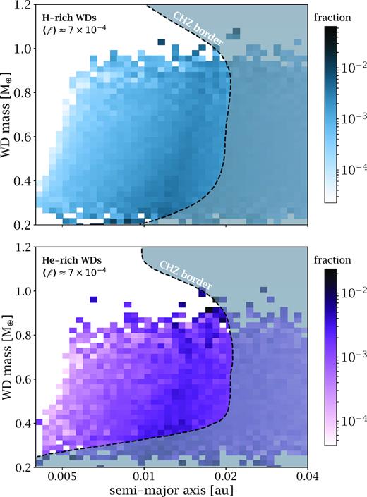
Top: Detectability of planets around H-rich WDs with LSST via transits. Injected planets are log-uniformly distributed in radius from 0.5 to 1.5 R_⊕ representing terrestrial planets, many of which reside inside (to left of) the outer edge of the CHZ marked by the dashed line. Bottom: Same as top except for He-rich WDs. Average detection fraction within the CHZ is shown in the upper left for both.

Open in new tabDownload slide

We briefly remark that the detectability rates are in the range of 10⁻² to 10⁻⁴, with the inner edge becoming attenuated due the impact of tidal disruption. This suggests that if the occurrence rate of CHZ rocky planets around WDs is η ≳ 10⁻³, we should anticipate detections with LSST.

4 DISCUSSION

We have demonstrated that LSST will have the capability to detect transiting planets around white dwarfs. Over an assumed 10 yr baseline, the sporadic sampling of LSST combines together to provide the excellent phase coverage needed for successful transit detection (also see Jacklin et al. 2015, 2017; Lund et al. 2015). Furthermore, LSST’s short integration time of 15 s ensures that WD transits, which typically last for a minute or two, are not significantly distorted due to binning (Kipping 2010) aiding their identification. These two advantages enable detection but it is LSST’s incredible depth, exceeding m_r = 25, which makes LSST potentially a revolution in the quest to detect WD planets since the survey will observe ∼10⁷ WDs.

We find that detection rates for P < 10 d planets range from 10⁻⁶ for long-period Ceres-sized bodies to 10⁻² for short-period Jovians. Rates are naturally highly dependent upon what type of planet is under consideration but our suite of results are made available at the previously mentioned github repository. Yield estimates are not directly possible due to our lack of information about the WD planet population. However, as an example we highlight that if η = 10 per cent of WDs host a Mars-sized planet with P < 10 d, we should expect ∼100 detections with LSST, and thus one might reasonably expect hundreds of discoveries.

If terrestrial planets reside in the continuous habitable zones of WDs with a frequency greater than η ≳ 10⁻³, LSST should be expected to detect examples. Assuming again η = 10 per cent would yield ∼100 detections. We would expect the brightest planet hosting WD in such an example to be m_r ∼ 18–22 and thus may be suitable for atmospheric characterization with JWST (Loeb & Maoz 2013).

We highlight some limitations of our study. First, our work assumes that the transit detection pipeline acts as a perfect detector for S/N > 7.1 and thus we did not execute blind recoveries of injected signals. Although typical search algorithms are found to have high efficiencies in this regime (e.g. see Christiansen et al. 2016), white dwarfs have not been surveyed in great detail before. Secondly, we assume long-term photometric behaviour is filterable and that short-term variations have an amplitude less than the formal uncertainties. Given the faintness of our targets, we argue this is a reasonable approximation where photon noise dominates. Finally, we highlight that whether a planet in the CHZ is truly habitable is a completely different question that we make no attempt to investigate in this work.

Ultimately, our work makes a strong case that although LSST may not have been built with WD transits as a science case in mind, it is uniquely placed to conduct the most in-depth survey to date. A preliminary survey with K2 of 1148 WDs by Van Sluijis & Van Eylen (2018) found no transiting objects and placed upper limits on planet occurrence rates in the range of η = 25 per cent to η = 95 per cent for 4 h to 10 d roughly Earth-sized bodies. For comparison, if LSST failed to detect similar objects, the occurrence rate would be constrained to be η ≲ 0.05 per cent. With prior indications of planetary material falling onto ∼30 per cent of WDs (Zuckerman et al. 2003, 2010; Koester et al. 2014), a search for minor bodies around such stars is both timely and critical for advancing our understanding of these intriguing environments.

SUPPORTING INFORMATION

WDplanets-master

Please note: Oxford University Press is not responsible for the content or functionality of any supporting materials supplied by the authors. Any queries (other than missing material) should be directed to the corresponding author for the article.

ACKNOWLEDGEMENTS

DK is supported by the Alfred P. Sloan Foundation. JC gratefully acknowledges the support of the Columbia University Bridge to Ph.D. Program in the Natural Sciences and the support provided by the National Science Foundation through grant AST-1539931. Special thanks to Scott Daniel for his guidance with using catsim and to Jay Farihi for his helpful comments on this work. Thanks to the members of the Cool Worlds Lab for regular discussions and feedback during the preparation of this work, and to the referee for a thorough and thoughtful review.

Footnotes

REFERENCES