


Abstract
Modifications of the matter power spectrum due to baryonic physics are one of the major theoretical uncertainties in cosmological weak lensing measurements. Developing robust mitigation schemes for this source of systematic uncertainty increases the robustness of cosmological constraints, and may increase their precision if they enable the use of information from smaller scales. Here we explore the performance of two mitigation schemes for baryonic effects in weak lensing cosmic shear: the principal component analysis (PCA) method and the halo-model approach in hmcode. We construct mock tomographic shear power spectra from four hydrodynamical simulations, and run simulated likelihood analyses with cosmolike assuming LSST-like survey statistics. With an angular scale cut of ℓmax < 2000, both methods successfully remove the biases in cosmological parameters due to the various baryonic physics scenarios, with the PCA method causing less degradation in the parameter constraints than hmcode. For a more aggressive ℓmax = 5000, the PCA method performs well for all but one baryonic physics scenario, requiring additional training simulations to account for the extreme baryonic physics scenario of Illustris; hmcode exhibits tensions in the 2D posterior distributions of cosmological parameters due to lack of freedom in describing the power spectrum for |$k \gt 10\ h^{-1}\, \mathrm{Mpc}$|. We investigate variants of the PCA method and improve the bias mitigation through PCA by accounting for the noise properties in the data via Cholesky decomposition of the covariance matrix. Our improved PCA method allows us to retain more statistical constraining power while effectively mitigating baryonic uncertainties even for a broad range of baryonic physics scenarios.
1 INTRODUCTION
The origin of the accelerated expansion of the Universe has been one of the most profound mysteries in modern cosmology since its discovery (Riess et al. 1998; Perlmutter et al. 1999). The Λ cold dark matter (ΛCDM) framework is currently consistent with observations of the expansion history of our Universe from early (Planck Collaboration XIII 2016) to late times (Abbott et al. 2018). Ongoing photometry surveys such as KiDS (Kilo-Degree Survey1), HSC (Hyper Suprime-Cam2), and DES (Dark Energy Survey3) or future experiments such as LSST (Large Synoptic Survey Telescope4), Euclid,5 and WFIRST (Wide-Field Infrared Survey Telescope6) experiments aim to constrain cosmological parameters to higher precision and search for deviations from ΛCDM in order to understand the nature of dark energy and general relativity.
Weak gravitational lensing (WL), the deflection of light by the gravitational potential of cosmic structure, is one of the most promising cosmological probes to discriminate between dark energy models (Weinberg et al. 2013; Mandelbaum 2018). Tomographic WL measurements, in which galaxy shapes are cross-correlated within and across bins in redshift space (e.g. Hu & Jain 2004), are directly sensitive to structure growth, with secondary dependence on the relative distance ratios. In order to use tomographic WL measurements to constrain cosmological parameters, an accurate model for matter density power spectrum, Pδ(k, z), is required. It has been estimated that Pδ(k, z) must be predicted to approximately 1 per cent accuracy for |$k \le k_{\rm max} \sim 10 \ h^{-1}\, \mathrm{Mpc}$| in order to avoid biasing cosmological parameter constraints in the era of LSST (Huterer & Takada 2005; Eifler 2011; Hearin, Zentner & Ma 2012).
In the linear and quasi-linear regimes, perturbation theory can be used to calculate the matter power spectra for a set of given cosmological parameters (Bernardeau et al. 2002). On smaller scales, N-body simulations are needed in order to capture the complicated non-linear evolution of structure growth. For example, the halofit method employs a functional form of Pδ(k, z) derived from halo models, and calibrates the model parameters from N-body simulations at various cosmological parameters (Smith et al. 2003; Takahashi et al. 2012). Alternatively, the cosmic emu package emulates Pδ(k, z) by directly interpolating the N-body simulation results at a range of cosmological models (Heitmann et al. 2010, 2014; Lawrence et al. 2017). However, only gravitational physics is included in these dark-matter-only (DMO) simulations, which neglects any modification of the matter distribution due to baryonic physics processes such as star formation, radiative cooling, and feedback (e.g. Cui, Borgani & Murante 2014; Velliscig et al. 2014; Mummery et al. 2017). These processes can modify Pδ(k, z) by tens of per cent compared to the DMO power spectra from k ≈ 1 to 10 |$\ h^{-1}\, \mathrm{Mpc}$| at z = 0 (van Daalen et al. 2011). The changes in the matter power spectrum due to baryonic physics can affect our inferences on dark energy (e.g. Copeland, Taylor & Hall 2018) and neutrino mass parameters (e.g. Harnois-Déraps et al. 2015) as they have similar effects on part of the power spectrum, but the different scale and redshift dependences can help in breaking some of the degeneracies.
There are several approaches to mitigating the impact of uncertainty in how the baryonic physics modifies the matter power spectrum. The simplest approach is to eliminate data points that may be severely affected by this uncertainty, so that limitations in small-scale modelling do not bias the inferred cosmology [e.g. see Krause et al. (2017) for the determination of the redshift-dependent angular scale cuts for the DES-Y1 analysis or see Taylor, Bernardeau & Kitching (2018) for another method relating angular scale cuts to physical (k) space]. This approach results in a loss of cosmological constraining power, especially when the statistical precision of the data increases in the future, resulting in the need for even more conservative scale cuts. A more economical way of discarding data is through peak clipping (Simpson et al. 2011; Simpson, Heavens & Heymans 2013). By cutting the most extreme peaks in the density fields of both observed and mock data sets, the derived summary statistics become less sensitive to the poorly modelled non-linear regime, while still allowing the use of a wider range of scales to extract cosmological information (Giblin et al. 2018). Eifler et al. (2015) propose the principal component analysis (PCA) framework (see also Kitching et al. 2016), which utilizes suites of hydrodynamical simulations to build a set of principal components (PCs) describing the modification of the observables by baryonic physics. The first few PC modes point towards directions in observable space where deviations from DMO power spectra due to baryons are most dominant. One can then efficiently remove the vast majority of baryonic uncertainties by discarding the first 3–4 PC modes. Mohammed & Gnedin (2018) point out that the training hydro simulations used to construct PCs have to be sufficiently broad in order to offer flexible degrees of freedom to span the possible baryonic scenarios for our Universe.
Other methods focus on modelling the ratio of power spectra that includes baryons to those that do not, with the goal of finding functional forms to describe the range of possible behaviour of Pδ,bary(k, z)/Pδ,DMO(k, z). Harnois-Déraps et al. (2015) use a parametric form with 15 parameters that is able to describe the power spectrum ratio of several OWLS simulations (van Daalen et al. 2011) to within 10 per cent precision up to |$k \approx 20 \ h^{-1}\, \mathrm{Mpc}$| and z < 1.5. Chisari et al. (2018) show that the above parametric form is sufficiently flexible to fit the power spectra ratio in the Horizon-AGN (Dubois et al. 2014) simulation to within 3 per cent across z ≲ 4 up to |$k \approx 30 \ h^{-1}\, \mathrm{Mpc}$|, but with the downside of involving too many free parameters. The authors propose a more compact model with four parameters that is capable of providing a fit to Horizon-AGN to within <5 per cent.
Based on the fact that baryonic physics mainly affects the matter power spectrum by altering the structure of dark matter haloes, another proposed approach is to model the deviations in the matter power spectrum through the framework of the halo model (Peacock & Smith 2000; Seljak 2000; Cooray & Sheth 2002). Zentner, Rudd & Hu (2008) and Zentner et al. (2013) demonstrate that incorporating the halo concentration–mass relation and its redshift evolution into the halo model framework and marginalizing over the associated free parameters can successfully mitigate baryonic bias for Stage III surveys such as DES, but is insufficient for Stage IV experiments. In addition to the degree of freedom that governs halo concentration, Mead et al. (2015, 2016) consider a parameter that characterizes the mass dependence of feedback, with publicly available software available for this model in hmcode.7 Copeland et al. (2018) further extend hmcode, introducing a core radius parameter to characterize the inner halo structure that is believed to be an outcome of baryonic effects (Martizzi et al. 2012). There are also approaches that go beyond NFW (Navarro–Frenk–White, Navarro, Frenk & White 1996) halo profiles, focusing on modelling the radial density distributions of stellar, gas, and DM components of haloes to capture the main features of baryonic feedback (Semboloni et al. 2011; Semboloni, Hoekstra & Schaye 2013; Mohammed et al. 2014; Schneider & Teyssier 2015; Schneider et al. 2019). The improvement of the halo model approach is an active research area, in particular on constraining the prior range. These halo model approaches potentially enable us to jointly constrain halo structural information and cosmological parameters from data.
Baryonic effects can be mitigated also via a joint analysis through optimized combination of different cosmological probes, as demonstrated in Osato, Shirasaki & Yoshida (2015). Finally, a gradient-based method is proposed recently by Dai, Feng & Seljak (2018). Dark matter particles in N-body simulations are moved along the gradient of estimated thermal pressure to mimic the effect of baryonic feedback. This method can be implemented as a post-processing step on N-body simulations to produce fast hydrodynamical-like simulations.
In this paper, we focus on studying two of the above baryonic mitigation methods – the PCA method and hmcode. We test the effectiveness of these baryonic physics mitigation techniques on a broad range of possible baryonic scenarios by applying them to LSST-like mock observables constructed from hydrodynamical simulations of MassiveBlack-II (Khandai et al. 2015), Illustris (Vogelsberger et al. 2014), Eagle (Schaye et al. 2015), and Horizon-AGN (Dubois et al. 2014), and comparing their cosmological parameter constraints. In addition, for the PCA method, we investigate different ways of constructing the PCs, and provide a modification to the original formalism to improve their efficiency.
This paper is organized as follows. In Section 2, we give an overview on the hydrodynamical simulations used in this work for the construction of our training and test sets. Section 3 describes the set-up of our simulated LSST-like likelihood simulations. In Section 4, we provide the detailed theoretical formalism for the baryonic mitigation techniques from literature and our improved PCA scheme applied in this work. Section 5 presents the main results of the likelihood simulations under various baryonic scenarios and compares the performances of different mitigation methods. We summarize our findings in Section 6, and discuss the prospects of PCA-based methods for future investigation.
2 BARYONIC EFFECTS IN SIMULATIONS
In this section, we introduce the hydrodynamical simulations involved in our analysis (summarized in Table 1), and compare the impact of the baryonic physics considered on the matter distributions.
Basic information for the hydrodynamical simulations used in this work.
| Simulation | Box length | Total | DM particle | Initial gas | Force softening | Cosmology |
|---|---|---|---|---|---|---|
| particle # | mass | particle mass | length | |||
| OWLS | 100 |$\ h^{-1}\, \mathrm{Mpc}$| | 2 × 5123 | |$4.06 \times 10^8 \ h^{-1}\, \mathrm{M}_{\odot }$| | |$8.66 \times 10^7 \ h^{-1}\, \mathrm{M}_{\odot }$| | 0.78 |$\ h^{-1}\, \mathrm{kpc}$| | WMAP3 |
| MassiveBlack-II | 100 |$\ h^{-1}\, \mathrm{Mpc}$| | 2 × 19723 | |$1.1 \times 10^7 \ h^{-1}\, \mathrm{M}_{\odot }$| | |$2.2 \times 10^6 \ h^{-1}\, \mathrm{M}_{\odot }$| | 1.85 |$\ h^{-1}\, \mathrm{kpc}$| | WMAP7 |
| Illustris | 75 |$\ h^{-1}\, \mathrm{Mpc}$| | 2 × 18203 | |$4.41 \times 10^6 \ h^{-1}\, \mathrm{M}_{\odot }$| | |$8.87 \times 10^5 \ h^{-1}\, \mathrm{M}_{\odot }$| | 1.4 |$\ h^{-1}\, \mathrm{kpc}$| | WMAP7 |
| Eagle | 67.77 |$\ h^{-1}\, \mathrm{Mpc}$| | 2 × 15043 | |$6.57 \times 10^6 \ h^{-1}\, \mathrm{M}_{\odot }$| | |$1.23 \times 10^6 \ h^{-1}\, \mathrm{M}_{\odot }$| | 1.8 |$\ h^{-1}\, \mathrm{kpc}$| | Planck2013 |
| Horizon-AGN | 100 |$\ h^{-1}\, \mathrm{Mpc}$| | 2 × 10243 | |$1.1 \times 10^7 \ h^{-1}\, \mathrm{M}_{\odot }$| | |$2.2 \times 10^6 \ h^{-1}\, \mathrm{M}_{\odot }$| | 1.85 |$\ h^{-1}\, \mathrm{kpc}$| | WMAP7 |
2.1 OWLS simulation suite
The OWLS simulations are a large suite of cosmological hydrodynamical simulations with varying implementations of subgrid physics to enable investigations of the effects of altering or adding a single physical process on the total matter distribution (Schaye et al. 2010). Here we adopt nine different baryonic simulations from OWLS. We refer readers to van Daalen et al. (2011) for a more detailed description.
REF: The baseline simulation that contains many of the physical processes known to be important for galaxy formation except for the active galactic nucleus (AGN) feedback mechanism. REF includes prescriptions of radiative cooling and heating for 11 different elements, star formation assuming the Chabrier (2003) stellar initial mass function (IMF), stellar evolution, mass-loss, chemical enrichment, and SN feedback in kinetic form (wind mass loading factor η = 2 and initial wind velocity vw = 600 km s−1 ; all together |$\eta v_{\rm w}^2$| determines the energy injected into the winds per unit stellar mass). The other eight hydro simulations are based on REF, with modifications indicated below.
NOSN: Exclude SN feedback.
NOZCOOL: Exclude metal-line cooling. Only assume primordial abundances when computing cooling rates.
NOSN_NOZCOOL: Exclude both SN feedback and metal-line cooling.
WML1V848: Adopt the same SN feedback energy per unit stellar mass as for REF, but reduce the mass loading factor by a factor of 2 (η = 1) and increase the wind velocity by a factor of |$\sqrt{2}$| (vw = 848 km s−1).
WDENS: Adopt the same SN feedback energy per unit stellar mass as that of REF, but let η and vw depend on gas density (|$v_{\rm w} \propto n_{\rm H}^{1/6}$|; |$\eta \propto n_{\rm H}^{-1/3}$|).
WML4: Double SN feedback per unit stellar mass by increasing the mass loading factor by a factor of 2 (η = 4).
DBLIMFV1618: Once the gas reaches a certain pressure threshold, 10 per cent of the star formation activity follows a top-heavy IMF. In this case, more high-mass stars are produced, which leads to higher SN energy feedback.
AGN: In addition to physics included in the REF model, add a subgrid model for BH evolution and AGN feedback following the prescription of Booth & Schaye (2009). BHs inject 1.5 per cent of the rest-mass energy of the accreted gas into the surrounding matter in the form of heat.
The simulation cube for OWLS is |$L = 100 \ h^{-1}\, \mathrm{Mpc}$| in comoving scale on a side. The OWLS-DMO simulation contains 5123 collisionless DM particles; the nine hydro simulations contain an additional 5123 particles in the form of collisional gas or collisionless stars to capture the baryonic processes. The DM and (initial) gas particle masses are |$\approx 4.06 \times 10^8$| and |$8.66 \times 10^7 \ h^{-1}\, \mathrm{M}_{\odot }$|, respectively. The gravitational softening length is |$\epsilon \approx 0.78 \ h^{-1}\, \mathrm{kpc}$| in comoving scale, and is limited to a maximum physical scale of |$2 \ h^{-1}\, \mathrm{kpc}$|. The cosmological parameters used in the simulation are based on WMAP3 results (Spergel et al. 2007): {Ωm, Ωb, ΩΛ, σ8, ns, h} = {0.238, 0.0418, 0.762, 0.74, 0.951, 0.73}.
The OWLS simulation sets are not specifically fine-tuned to match with key observables. As indicated in McCarthy et al. (2017), the original OWLS models underpredict the abundance of |$M_* \lt 10^{11} \, \mathrm{M}_{\odot }$| galaxies at the present day due to overly efficient stellar feedback (see their fig. 1). The successor BAHAMAS simulation lowers the wind velocity vw from 600 to 300 km s−1 in order to provide a better fit to the observed abundance of low-to-intermediate-mass galaxies.8
2.2 Eagle simulation
The Eagle simulation (Schaye et al. 2015) is conducted in a cubic periodic box of side length |$L = 67.77 \ h^{-1}\, \mathrm{Mpc}$| (comoving). There are 15043 DM particles in both hydrodynamical and DMO simulations, and an approximately equal number of baryonic particles in the hydrodynamical run. The mass of each DM particle is |$6.57 \times 10^6 \ h^{-1}\, \mathrm{M}_{\odot }$| and the initial baryonic mass resolution is |$1.23 \times 10^6 \ h^{-1}\, \mathrm{M}_{\odot }$|. The gravitational softening length is |$\epsilon = 1.8 \ h^{-1}\, \mathrm{kpc}$| in comoving units (The EAGLE team 2017). The cosmological parameters used in Eagle are consistent with Planck 2013 results (Planck Collaboration XVI 2014): {Ωm, Ωb, ΩΛ, σ8, ns, h} = {0.307, 0.04825, 0.693, 0.8288, 0.9611, 0.6777}.
The subgrid physics used in Eagle is based on OWLS. The physical models include radiative cooling and photoionization heating; star formation associated with stellar mass-loss and energy feedback; BH mergers, gas accretion, and AGN feedback. The most important changes compared to OWLS are: star-forming feedback energy changing in terms of thermal form rather than kinetic; accounting for angular momentum during the accretion of gas onto BHs; inclusion of a metallicity-dependence in the star formation law. In contrast to many hydrodynamical simulations, Eagle employs stellar and AGN feedback only in thermal form, which captures the collective effects of mechanisms such as stellar winds, radiation pressure, SN feedback, and radio- and quasar-mode AGN feedback. One major improvement in the treatment of thermal feedback is that it can be performed without turning off radiative cooling and hydrodynamical forces.
The galaxy stellar mass function of Eagle matches extremely well with observations at z = 0.1, because its stellar and AGN feedback related parameters are specifically calibrated at each resolution to reproduce this observable (see Crain et al. 2015; Schaye et al. 2015 for details of calibration philosophy).
2.3 MassiveBlack-II simulation
The MassiveBlack-II (hereafter MB2) simulation is a high-resolution ΛCDM cosmological simulation (Khandai et al. 2015). Both DMO (Tenneti et al. 2015) and hydrodynamical MB2 simulations are conducted in a cubic simulation box with sides of length |$L = 100 \ h^{-1}\, \mathrm{Mpc}$| in comoving scale. There are 19723 DM particles in both the MB2-hydro and MB2-DMO simulations, with an additional 19723 initial number of gas particles in the hydro run. The mass of each DM particle is |$1.1 \times 10^7 \ h^{-1}\, \mathrm{M}_{\odot }$| and the initial baryonic mass resolution is |$2.2 \times 10^6 \ h^{-1}\, \mathrm{M}_{\odot }$|. The gravitational softening length is |$\epsilon = 1.85 \ h^{-1}\, \mathrm{kpc}$| in comoving units. The cosmological parameters in MB2 are consistent with WMAP7 results (Komatsu et al. 2011): {Ωm, Ωb, ΩΛ, σ8, ns, h} = {0.275, 0.046, 0.725, 0.816, 0.968, 0.701}.
The subgrid models of baryonic physics in MB2 include a multiphase interstellar medium model with star formation and associated feedback by SN and stellar winds (Springel & Hernquist 2003); BH accretion, merger, and associated AGN feedback in quasar-mode (Di Matteo, Springel & Hernquist 2005; Springel, Di Matteo & Hernquist 2005).
The AGN feedback efficiency of MB2 is relatively weak compared with other hydrodynamical simulations that have AGN subgrid physics involved in this work. One outcome of this is that MB2 overpredicts the abundance of massive galaxies at low redshift (Khandai et al. 2015).
2.4 Illustris simulation
The Illustris simulation (Vogelsberger et al. 2014) is carried out in a cubic periodic box with sides of length |$L = 75 \ h^{-1}\, \mathrm{Mpc}$| (comoving). We download the highest resolution snapshot data from the public release website (Nelson et al. 2015) to calculate power spectra for both hydrodynamical and DMO runs. There are 18203 DM particles in both hydrodynamical and DMO simulations, and an approximately equal number of baryonic particles in the hydrodynamical run. The mass of each DM particle is |$4.41 \times 10^6 \ h^{-1}\, \mathrm{M}_{\odot }$| and the initial baryonic mass resolution is |$8.87 \times 10^5 \ h^{-1}\, \mathrm{M}_{\odot }$|. The gravitational softening length is |$\epsilon = 1.4 \ h^{-1}\, \mathrm{kpc}$| in comoving units. The cosmological parameters adopted in Illustris are consistent with WMAP7 results (Komatsu et al. 2011): {Ωm, Ωb, ΩΛ, σ8, ns, h} = {0.2726, 0.0456, 0.7274, 0.809, 0.963, 0.704}.
Illustris incorporates a broad range of galaxy formation physics (Vogelsberger et al. 2013): gas cooling in primordial and metal-lines; stellar evolution associated with chemical enrichment and stellar mass-loss; kinetic stellar feedback driven by SN; BH accretion, merging, and related AGN feedback in terms of quasar- and radio-modes as well as associated radiative electromagnetic feedback.
Illustris is run using the moving-mesh-based code arepo (Springel 2010), which is more efficient in cooling compared with classical particle-based SPH codes (e.g. Springel 2005). The energy input from feedback is designed to be strong to avoid efficient stellar mass build-up. Even with this setting, Illustris still overshoots the observed low-redshift stellar mass function on both high- and low-mass ends. The radio-mode AGN feedback is also too violent for the gas component, under predicting the baryon content in lower redshift high-mass haloes where the radio-mode feedback is the dominant heating channel (Genel et al. 2014; Haider et al. 2016). The successor IllustrisTNG simulation replaces the intense thermal energy dump of radio-mode feedback with kinematic kicks to heat up affected gas particles (Weinberger et al. 2018).
2.5 Horizon-AGN simulation
The Horizon-AGN (Dubois et al. 2014) is carried out in a cubic periodic box of side length |$L = 100 \ h^{-1}\, \mathrm{Mpc}$| (comoving). There are 10243 DM particles in both the DMO and hydrodynamical runs, with the DM particle mass of |$9.9 \times 10^7 \ h^{-1}\, \mathrm{M}_{\odot }$| for the DMO run, and |$8.3 \times 10^7 \ h^{-1}\, \mathrm{M}_{\odot }$| for the hydrodynamical run. The initial gas particle mass is about |$1 \times 10^7 \ h^{-1}\, \mathrm{M}_{\odot }$|. The cosmological parameters used in the simulation are compatible with WMAP7 cosmology (Komatsu et al. 2011): {Ωm, Ωb, ΩΛ, σ8, ns, h} = {0.272, 0.045, 0.728, 0.81, 0.967, 0.704}.
Subgrid physics models for a variety of baryonic physics effects are implemented in Horizon-AGN. Gas is allowed to cool down to 104 K via transition lines of hydrogen and helium as well as metals using the Sutherland & Dopita 1993 model. When the hydrogen number density exceeds a threshold of |$0.1\,\rm {H}\,\rm {cm}^{-3}$|, star formation is triggered following a random Poisson process (Shandarin & Zeldovich 1989; Rasera & Teyssier 2006). SN feedback is taken into account assuming an IMF with a low-mass cut-off at 0.1 M⊙ and a high-mass cut-off at 100 M⊙. Chemical enrichment happens along with SN explosions and stellar winds. The AGN feedback is modelled in a combination of two different modes: the kinematic radio mode when |$\dot{M}_{\rm BH} / \dot{M}_{\rm Edd} \lt 0.01$| and the thermal quasar mode otherwise (Dubois et al. 2012).
Although Horizon-AGN is not specifically tuned to reproduce the galaxy stellar mass function at local Universe, it shows reasonable consistency with observations, with slight overproduction of galaxies at the low-mass end (Kaviraj et al. 2017).
2.6 Comparison of power spectra in hydrodynamical versus DMO simulations
From the snapshot data release of Eagle, MB2, and Illustris, we calculate the matter power spectra as detailed in Appendix A. For OWLS and Horizon-AGN simulations, we use the computed results from van Daalen et al. (2011) and Chisari et al. (2018), respectively. Power spectra from DMO simulations, with the same initial condition as their paired hydrodynamical simulations, are also computed in order to perform a fair comparison across simulations with different cosmological parameters and with reduced cosmic variance. For each paired simulation set, only a single realization was available to construct the power spectrum ratio.
Fig. 1 shows the z = 0 ratio of power spectra from different hydrodynamical simulations with respect to their counterpart DMO simulations. The thin lines indicate the nine different baryonic scenarios in the OWLS simulation suite. For the eight baryonic scenarios without AGN feedback, the common feature is a rapid increase in power on small scales. The power enhancement is due to efficient cooling of gas which eventually leads to the formation of galaxies within haloes, and further concentrates the DM distribution (Blumenthal et al. 1986). Simulations without SN feedback (NOSN, NOSN_NOZCOOL) tend to have an even stronger increase in power compared to the reference simulation REF due to the enhanced cooling effect. When adding AGN feedback to REF, the power is suppressed dramatically, with 1 per cent reduction for |$k \approx 0.3 \ h^{-1}\, \mathrm{Mpc}$| and exceeding 10 per cent for |$k \gtrsim 2 \ h^{-1}\, \mathrm{Mpc}$| (van Daalen et al. 2011). The suppression of power is due to baryons being pushed outward by the energetic AGN feedback processes.
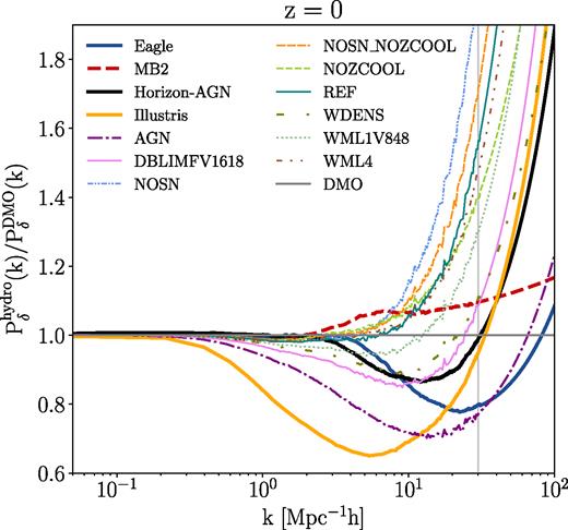
The ratios of the matter power spectra in different hydrodynamical simulations with respect to their counterpart DMO simulations at z = 0. The thick lines show results for the Eagle, MB2, and Illustris simulations, while the thin lines indicate the nine different baryonic scenarios in OWLS simulation suite. The grey vertical line separates between regions where the data points come from direct measurement (|$k \lesssim 30 \ h^{-1}\, \mathrm{Mpc}$|) and from extrapolation with a quadratic spline fit (|$k \gtrsim 30 \ h^{-1}\, \mathrm{Mpc}$|; see Appendix B for further details).
The thick lines represent power spectra ratio for Eagle, MB2, Illustris, and Horizon-AGN simulations. Although they all involve a broad range of astrophysical processes that are believed to be relevant to galaxy formation, the resulting power spectra show significant differences. The feedback mechanism in Illustris drastically suppresses the power by 35 per cent at |$k \approx 5 \ h^{-1}\, \mathrm{Mpc}$|. Eagle reaches its maximum suppression of power of 20 per cent at |$k \approx 20 \ h^{-1}\, \mathrm{Mpc}$|. A similar trend is also observed in Horizon-AGN, but it reaches its minimum amplitude reduction of 10 per cent at |$k \approx 10 \ h^{-1}\, \mathrm{Mpc}$|. Going towards higher k, we start to see that the ratio curves bend upward and keep increasing beyond k of |$30 \ h^{-1}\, \mathrm{Mpc}$|. The MB2 power spectrum behaves relatively similar to DMO, but still the baryonic prescription prevents the power spectrum ratio from growing too quickly compared to the OWLS scenarios without AGN feedback, which suffer from severe overcooling effect (e.g. Tornatore et al. 2003; McCarthy et al. 2011).
Equation (1) illustrates the most important assumption in this work: we assume that baryonic effects on the power spectrum can be represented as a fractional change in the power spectrum, and that this fractional change is independent of cosmology. The cosmology enters our analysis only through the theoretical power spectrum |$P_{\delta }^{\rm theory}(k, z\ |\ \boldsymbol p_{\rm co})$|. This is a reasonable assumption. According to van Daalen, McCarthy & Schaye (2019), the power spectrum ratio remains more or less the same when varying cosmologies (see their fig. 6).
3 LIKELIHOOD ANALYSIS METHODOLOGY
Here we present our methodology in estimating the cosmological constraining power for an LSST-like survey. We start by describing the theoretical models used in the work, our mock observations, the covariance matrix constructed for an LSST-like survey, and finally the likelihood formalism used in estimating the posterior distribution of cosmological parameters. The cosmological model considered in our likelihood simulation is flat wCDM, with varying cosmological parameters |$\boldsymbol p_{\rm co}=\lbrace \Omega _{\mathrm{m}},\ \sigma _8,\ \Omega _{\mathrm{b}},\ n_{\mathrm{s}},\ w_0,\ w_{\rm a},\ h\rbrace$|.
3.1 Theoretical models
We rely on two main theoretical models to fit our mock observables in this work. The first one is the Takahashi et al. (2012) version of halofit. It adopts empirically motivated functional forms to characterize the variation of power spectra with cosmology. Having been calibrated with high-resolution N-body simulations, it provides an accurate prediction of the non-linear matter spectrum with 5 per cent precision at |$k \le 1 \ h^{-1}\, \mathrm{Mpc}$| and 10 per cent at |$1 \le k \le 30 \ h^{-1}\, \mathrm{Mpc}$| within the redshift range of 0 ≤ z ≤ 10.
The second fitting routine is hmcode, constructed by M15. It utilizes the halo-model formalism to describe the cosmological change of power spectra via physically motivated parameters. hmcode has prescriptions for capturing the impact of baryons on the matter power spectrum via two free parameters: the amplitude of the concentration–mass relation (A; see equation 14 in M15), and a halo bloating parameter (η0; see equations 26 and 29 in M15) controlling the change of dark matter halo profiles in a halo mass-dependent way to account for different feedback energy levels. When allowing A and η0 to vary, it can successfully fit the power spectra from various baryonic scenarios of OWLS (M15). When fixing A = 3.13 and η0 = 0.6044, hmcode functions as a regular DMO-based emulator, which is calibrated with high-resolution N-body simulations to an accuracy of |$\approx 5{{\ \rm per\ cent}}$| at |$k \le 10 \ h^{-1}\, \mathrm{Mpc}$| for z ≤ 2. We note that the |$\approx 5{{\ \rm per\ cent}}$| discrepancy between the DMO mode of hmcode and halofit is non-negligible within LSST statistics. We therefore construct two sets of mock observables based on each theoretical model.
3.2 Mock observational data
We rely on four hydrodynamical simulations: Eagle, MB2, Illustris, and Horizon-AGN to construct mock observables, and investigate the performances of the PCA method (Eifler et al. 2015, hereafter E15) and the halo model approach (Mead et al. 2015, hereafter M15) on mitigating baryonic effects. These methods will be described in more detail in Section 4. For simplicity, besides baryonic effects, our mock data vectors do not include any other source of noise or systematics.
We perform a tomographic analysis by dividing the sources into 10 tomographic bins with equal total number of galaxies in each bin. We also smooth the redshift distribution with a Gaussian kernel to characterize potential photo-z uncertainties. Fig. 2 shows the exact redshift distribution in each bin. This results in 55 unique combinations of auto- and cross-correlation shear tomographic power spectra. For each of the tomographic power spectra, we consider 18 equally spaced logarithmic bins in angular wavenumber ℓ ranging from 23 to 2060. This results in a total of 55 × 18 = 990 data points in our data vector. For the main analysis of this paper, we adopt an upper limit of ℓmax ≈ 2000. This limit is driven by the resolution of the hydrodynamical simulations used in this work. We refer readers to Appendix B for further details on how we extrapolate power spectra to perform the integration to derive Cij(ℓ), and how the decision on the ℓmax ≈ 2000 cut is made.
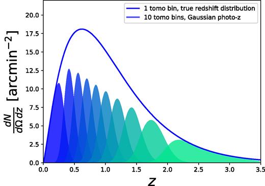
The normalized galaxy number density split into 10 Gaussian tomographic photo-z bins as shaded regions from blue (low z) to green (high z). For comparison, we show the true underlying redshift distribution as a solid blue line.
The fiducial cosmology |$\boldsymbol p_{\rm co, fid}$| of the data vectors is set to be consistent with the Planck 2015 (TT+TE+EE+lowP and assuming ΛCDM) results (Planck Collaboration XIII 2016) as summarized in Table 2.
Fiducial cosmology, minimum and maximum of the flat prior on the cosmological parameters, and halo-structural parameters in hmcode.
| Parameter | Fiducial | Prior |
|---|---|---|
| Ωm | 0.3156 | Flat (0.05, 0.6) |
| σ8 | 0.831 | Flat (0.5, 1.1) |
| ns | 0.9645 | Flat (0.84, 1.06) |
| w0 | −1.0 | Flat (−2.1, 0.0) |
| wa | 0.0 | Flat (−2.6, 2.6) |
| Ωb | 0.0049 | Flat (0.04, 0.055) |
| h0 | 0.6727 | Flat (0.4, 0.9) |
| A | – | Flat (0.5, 10) |
| η0 | – | Flat (0.1, 1.2) |
Our mock data vectors for various baryonic physics scenarios are computed with the Pδ term in equation (2) generated from equation (1). Since halofit and hmcode (in DMO mode) agree at the level of |$\lesssim 5{{\ \rm per\ cent}}$| to |$k = 10 \ h^{-1}\, \mathrm{Mpc}$|, and |$\lesssim 10{{\ \rm per\ cent}}$| out to |$k \le 100 \ h^{-1}\, \mathrm{Mpc}$| (see fig. 4 of M15), we create two sets of Eagle/MB2/Illustris/Horizon-AGN data vectors, with |$P_{\delta }^{\rm theory}(k, z\ |\ \boldsymbol p_{\rm co, fid})$| generated from halofit or hmcode, and incorporate the baryonic features through the power spectrum ratio. Throughout our experiment, when relying on halofit or hmcode as the theoretical model to perform fitting, we use the same fitting function to generate the mock observational data vectors for the fiducial cosmology. This way, when comparing the performance of different baryonic mitigation schemes, if one of the methods fails to recover the fiducial cosmological parameters, we can be assured that this failure is purely because of that method’s inability to mitigate the modification of the matter power spectrum due to baryonic physics, not because of an inherent discrepancy between the mock data and the DMO matter power spectrum model.
In Fig. 3 we show the ratio of baryonic to DMO |$C^{00}(\ell , \boldsymbol p_{\rm co, fid})$| shear power spectrum for various simulations. The thin lines indicate the nine baryonic scenarios from the OWLS simulation suite. The thick lines represent the Eagle/MB2/Illustris/Horizon-AGN universes, which are the data vectors that we will use for the LSST-like experiment. One can see that in this lowest tomographic bin, even for large scales at ℓ ≈ 100, the baryonic scenario of Illustris already causes a deviation from DMO at the 5 per cent level, with even more severe suppressions at smaller angular scales. For higher redshift tomographic bins, the deviations between hydrodynamical and DMO simulations are less severe. Semboloni et al. (2011) showed that a scale cut of ℓmax ≈ 500 would be needed to avoid w0 bias for a Euclid-like survey if the baryonic scenario of our Universe is like OWLS-AGN. When applying the traditional way of mitigating baryonic uncertainty by omitting small-scale information, we would need to discard a considerable amount of data before we can rely on DMO-based theoretical model to achieve an unbiased cosmological inference.
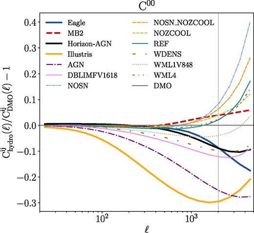
The ratio of tomographic shear power spectra of different hydrodynamical simulations with respect to their counterpart DMO simulations for the lowest auto-correlation tomographic bin with the cosmology set at the Planck 2015 result (Table 2). The thick lines represent the cases for Eagle/MB2/Illustris/Horizon-AGN simulations, while the thin lines indicate the nine different baryonic scenarios in OWLS simulation suite.
One subtle feature shown in Fig. 3 is that there is a small but noticeable large-scale excess of power (<0.4 per cent) in the Horizon-AGN simulation. This is because the power spectrum ratio between hydrodynamical and DMO runs of Horizon-AGN has <0.1 per cent excess at large scales (see Fig. 1), even though they share the same initial conditions. The true cause of this subtle excess is not clear. After exploring, Chisari et al. (2018) concluded that this may originate from the box being too small to reach the linear regime at large scales. However, the other simulations studied here are similar in size and do not exhibit this feature.
3.3 Covariance matrix
We generate the analytical covariance matrix of tomographic shear power spectra using cosmolike (Eifler et al. 2014; Krause & Eifler 2017). Briefly, our covariance matrix contains both Gaussian and non-Gaussian parts. The Gaussian covariance matrix contains contributions from cosmic variance and shape noise, derived under the assumption that the 4pt-function of the shear field can be expressed in terms of 2pt-functions (Hu & Jain 2004; Takada & Bridle 2007). The non-Gaussian part is given by the convergence trispectrum derived using the halo model (Cooray & Sheth 2002), which contains one-, two-, three-, and four-halo terms and a halo sample variance term characterizing the scatter of halo number density due to large-scale density fluctuations (Cooray & Hu 2001; Sato et al. 2009; Takada & Jain 2009). The exact equations of our implementation can be found in the appendix of Krause & Eifler (2017).
We assume 18 000 |$\rm {deg}^2$| as the survey area in our covariance matrix and adopt the same redshift distribution and source galaxy number density (|$26\,\rm {arcmin}^{-2}$|) as depicted in Fig. 2. The shape noise is set to be σϵ = 0.26 in each ellipticity component.
3.4 Likelihood formalism
We use the python emcee package (Foreman-Mackey et al. 2013), which relies on the algorithm of Goodman et al. (2010) to sample the parameter space spanned by |$\boldsymbol p_{\rm co}$| ({Ωm, σ8, Ωb, ns, w0, wa, h0}) as well as |$\boldsymbol p_{\rm nu}$| (if needed depending on the model). Altogether, we have conducted ∼250 likelihood simulations to present the results for this paper. The MCMC (Markov Chain Monte Carlo) chains contain ∼200 000 to 400 000 MCMC steps (after discarding 100 000 steps as burn-in phase), depending on the dimension of the parameter space that ranges from 7 to 16. For simplicity, we assume flat priors for all of our parameters, with their minimum and maximum values summarized in Table 2. For likelihood simulations with informative priors based on Planck, we refer readers to E15. Informative priors help to better constrain ns, Ωb, and h, to which cosmic shear is not very sensitive.
We will present in Section 4 on how we implement various baryonic mitigation schemes in the likelihood analysis. But before that, in Fig. 4 we show the posterior distribution of cosmological parameters derived from our LSST likelihood simulation, when naively applying the halofit model on fitting the data vectors contaminated with baryonic effects from Eagle/MB2/Horizon-AGN/Illustris simulations. For ease of visualization, we only show posteriors in the subspace of four cosmological parameters out of seven in total. Depending on the intensity of baryonic feedback as reflected in the ratio of hydrodynamical to DMO power spectra shown in Fig. 1, the resulting cosmology constraints can be severely biased in the case of Illustris (2σ–13σ depending on cosmological parameters) or at 1σ–2σ level in the other three cases. We note that the degree of bias depends on the ℓmax used in the analysis. Fig. 4 presents the result when applying a cut at ℓmax ≈ 2000 on |$\boldsymbol D$|, which is the default setting in the paper. In Section 5.4, we will show how this result changes when extending data vectors to ℓmax ≈ 5000.
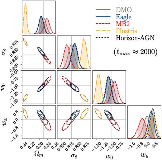
Cosmological parameter constraints for an LSST-like weak lensing survey with data vectors generated using various baryonic physics scenarios: pure DM (grey/solid) and the Eagle (blue/solid), MB2 (red/dashed), Illustris (yellow/dot–dashed), and Horizon-AGN (black/dotted) hydrodynamical simulations. In all cases, baryonic physics was ignored during the likelihood analysis, hence providing a worst-case scenario for biases due to baryonic physics. The analyses are carried out assuming non-informative priors on the parameters. Here, and in all such 2D posterior plots below, the contours depict the 68 per cent confidence levels. Depending on the intensity of the baryonic feedback, the resulting posterior distributions can be significantly away from the fiducial cosmology (marked in grey lines).
4 METHODS OF MITIGATING BARYONIC EFFECTS
In this section, we describe the methods used to mitigate the impact of baryonic physics on the cosmological parameter estimates from weak lensing. The methods can be classified into two categories: PCA-based methods and the halo-model-based approach. We discuss several PCA-based methods that are minor variants of each other in Sections 4.1–4.3. The halo-model based approach is described in Section 4.4. Throughout the work, we use the nine OWLS simulations as our ‘training sample’ to construct PCs for the PCA-based methods, and use the four mock data vectors constructed from Eagle/MB2/Illustris/Horizon-AGN simulations as ‘test sample’ to test methods listed in Table 3.
Summary of baryonic physics mitigation techniques. The first column is the label of each method, which we refer to in the text and plots throughout the work. The second column has simple descriptions that highlight the essential elements of each method. The third column presents the exact |$\boldsymbol \chi ^2$| equations that go into the likelihood analysis. Finally, the last column provides a section number where more information can be found for each method.
| Method | Brief description | χ2 equation | Section |
|---|---|---|---|
| reference | |||
| A | PCA in difference matrix, with exclusion | |$[(\boldsymbol D-\boldsymbol M)_{\rm pc, cut}]^{\rm t}\ \mathbf {C}^{-1}_{\rm pc, cut}\ [(\boldsymbol D-\boldsymbol M)_{\rm pc, cut}]$| | Section 4.1.1 |
| B | PCA in difference matrix, with marginalization | |$[\boldsymbol D-\boldsymbol M_B(\boldsymbol p_{\rm co}, \boldsymbol Q)]^{\rm t}\ \mathbf {C}^{-1}\ [\boldsymbol D-\boldsymbol M_B(\boldsymbol p_{\rm co}, \boldsymbol Q)]$| | Section 4.1.2 |
| C | PCA in |$\mathbf {L}^{-1}$| weighted difference matrix, with exclusion | |$[\mathbf {U}_{\rm ch} \mathbf {P}\mathbf {U}_{\rm ch}^{\rm t} \mathbf {L}^{-1}(\boldsymbol D-\boldsymbol M)]^{\rm t}\ \mathbf {I}\ [\mathbf {U}_{\rm ch} \mathbf {P}\mathbf {U}_{\rm ch}^{\rm t} \mathbf {L}^{-1}(\boldsymbol D-\boldsymbol M)]$| | Section 4.2 |
| D | PCA in fractional difference matrix, with marginalization | |$[\boldsymbol D-\boldsymbol M_R(\boldsymbol p_{\rm co}, {\boldsymbol Q})]^{\rm t}\ \mathbf {C}^{-1}\ [\boldsymbol D-\boldsymbol M_R(\boldsymbol p_{\rm co}, {\boldsymbol Q})]$| | Section 4.3 |
| M | Halo model parameter marginalization | |$[\boldsymbol D-\boldsymbol M_{\rm HMcode}(\boldsymbol p_{\rm co}, A, \eta _0)]^{\rm t}\ \mathbf {C}^{-1}\ [\boldsymbol D-\boldsymbol M_{\rm HMcode}(\boldsymbol p_{\rm co}, A, \eta _0)] \!\!\!\!\!\!$| | Section 4.4 |
4.1 PCA in difference matrix
4.1.1 Summary of the PCA framework (method A)
The original framework for using PCA to mitigate the impact of baryonic physics for weak lensing is described in Eifler et al. (2015). The essential idea is that even though hydrodynamical simulations with different baryonic prescriptions predict a range of variations on the matter power spectra (Fig. 1), we can still extract the common features of those diversity using PCA, and build an empirical model to mitigate baryonic uncertainty based on these hydrodynamical simulations. Below we provide a step-by-step description of the PCA framework.
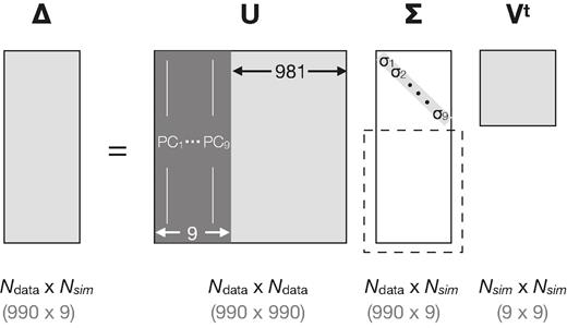
We perform SVD on the difference matrix |$\boldsymbol \Delta$| built based on the nine baryonic scenarios of OWLS (see equation 8). |$\mathbf {U}$| is a unitary matrix with columns that form an orthonormal basis set to span the 990-dimensional space of our data vector. Among them, the first nine PCs of |$\mathbf {U}$| form a complete description of the modifications of the data vector due to baryonic physics in the nine OWLS hydro simulations. We will test whether these nine PCs can also describe the impact of baryonic physics in the Eagle/MB2/Illustris/Horizon-AGN simulations.
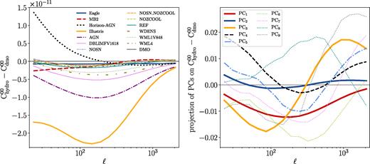
Left: The difference vectors, |$\boldsymbol B-\boldsymbol M$|, from the OWLS simulation set used to construct PCs as input in columns of equation (8). The thicker lines indicate the difference vectors for Eagle/MB2/Horizon-AGN/Illustris simulations as our test set. Right: The PC modes constructed from the OWLS simulation set in projection on the difference vector space for the tomographic bin C00. The goal of this work is to check whether these PC modes can flexibly describe the baryonic physics scenarios in the test set hydrodynamical simulations.
4.1.2 The marginalization version of the PCA framework (method B)
Theoretically, one can prove that the likelihood functions of equation (14) (method A) and equation (16) return identical results if the priors on the PC amplitudes are uninformative. We will provide comparisons of the posterior distributions of |$\boldsymbol p_{\rm co}$| in Section 5.1 and further comment on both methods there.
4.2 Noise-weighted PCA – Cholesky decomposition (method C)
As noted at the end of section 2.2 of E15, performing PCA on the difference matrix |$\boldsymbol \Delta$| (equation 8) is not necessarily the most optimal choice. They suggested an option of conducting the PCA on the ‘noise’-weighted |$\boldsymbol \Delta$|. As a result of re-weighting, the derived PCs would be more sensitive in accounting for deviations in data vectors due to baryonic physics at well-measured data points, where larger weighting factors are applied. Therefore, when doing PC mode removal, we tend to more effectively remove baryonic physics degrees of freedom that impact better-measured (lower noise) scales, which may more effectively reduce cosmological parameter biases.
 , which can be easily proved as follows:
In other words, after applying equation (18), we not only re-weight but also decorrelate the data vector.
In Fig. 7, we show the |$\boldsymbol B_{\rm ch} - \boldsymbol M_{\rm ch} = \mathbf {L}^{-1}(\boldsymbol B-\boldsymbol M)$| vectors in our lowest tomographic bin, at |$\boldsymbol p_{\rm co, fid}$|. The thicker lines represent our four test simulations; the thinner lines are for the nine baryonic scenarios in OWLS, which compose the columns of |$\boldsymbol \Delta _{\rm ch}$| in equation (20). Comparing with the left-hand panel of Fig. 6, one can see that after re-weighting by |$\mathbf {L}^{-1}$|, we more strongly emphasize baryonic fluctuations at smaller scales, so the PCs should also be more effective in accounting for small-scale baryonic features.9
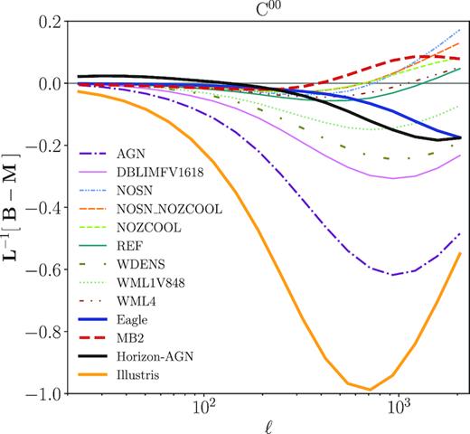
The discrepancy between baryon-contaminated data vectors and model in terms of |$\boldsymbol B_{\rm ch} - \boldsymbol M_{\rm ch}$| for various hydrodynamical simulations in the lowest tomographic bin. This is similar to the left-hand panel of Fig. 6, but here shows results for the case when applying Cholesky decomposition on our |$\boldsymbol B$| and |$\boldsymbol M$| vectors. The nine OWLS baryonic scenarios (thinner lines) compose columns of |$\boldsymbol \Delta _{\rm ch}$|, which are used to build PCs. These PCs are used to span the variation of Eagle/MB2/Illustris/Horizon-AGN simulations in |$\boldsymbol D_{\rm ch} - \boldsymbol M_{\rm ch}$| space. After Cholesky decomposition, the largest data-model inconsistency shifts to smaller scales compared with the upper panel of Fig. 6, indicating the PCs trained from |$\boldsymbol \Delta _{\rm ch}$| are more efficient at describing small-scale variations in the matter power spectrum due to baryonic physics compared with performing PCA on |$\boldsymbol \Delta$|.

4.3 PCA in fractional difference matrix (method D)
Similar to the concept mentioned in Section 4.2, performing PCs on the matrix |$\boldsymbol R$| can be viewed as putting the weight of |$1/\boldsymbol M$| into the PCA analysis. Since |$\boldsymbol M$| decreases with increasing ℓ, and the overall amplitude of |$\boldsymbol M$| increases towards higher redshift, after taking its inverse, we upweight data points at smaller scales and lower redshift. The fractional difference vectors of OWLS that go into columns of |$\boldsymbol R$| are plotted in Fig. 3. The PCs derived from |$\boldsymbol R$| are expected to be more efficient in accounting for smaller scale and lower redshift variation of the observables due to baryonic physics.
4.4 |$\rm{\small HMCODE}$| (method M)
Finally, we compare the above PCA-based methods with the halo model-based approach proposed by Mead et al. (2015), hmcode. hmcode utilizes two halo profile-related parameters to capture the impact of baryonic physics on the matter power spectrum: the amplitude of the concentration–mass relation (A) and a halo bloating parameter (η0) controlling the (mass-dependent) change of halo profiles. We refer readers back to Section 3.1 for a brief summary of this approach.
Equation (28) is derived based on the OWLS simulation suite. We will test whether it remains valid for the baryonic physics scenarios in Eagle/MB2/Illustris/Horizon-AGN for our forecasted scenario with LSST-like statistical power. Also, we will compare the performances of hmcode (marginalization over halo model parameters) with the above PCA-based methods.
5 PERFORMANCES OF BARYONIC MITIGATION TECHNIQUES
In this section, we present our simulated likelihood analysis for the different baryonic mitigation schemes listed in Table 3. We refer readers back to Section 3 for a description of the simulated likelihood analysis set-up.
Ideally, we need a baryonic physics mitigation strategy that can reduce the biases in cosmological parameters due to inaccuracies in theoretical modelling (as demonstrated in Fig. 4) to a level that is much smaller than the statistical uncertainties. In addition, we hope that the increase in statistical errors on cosmological parameters due to the additional nuisance parameters will be as small as possible. Throughout this section, we will use a criterion of bias <0.5σ (where σ represents the marginalized statistical error) for individual cosmological parameters to evaluate whether a method is effective in mitigating the uncertainties due to baryonic physics under various baryonic scenarios. We also compare their performance based on the degradation of cosmological constraining power through the size of the 1D marginalized uncertainties on cosmological parameters.
5.1 PC mode exclusion versus marginalizing over PC amplitude
We start by presenting the results for methods A and B (see Table 3) with their PCs described using the same difference matrix |$\boldsymbol \Delta$|. In method A, we modify the data vector by excluding the first few PC modes and modify the covariance self-consistently as well. In method B, the data vector and covariance matrix are unmodified, but we introduce free parameters describing the PC amplitudes to marginalize over in the likelihood analysis.
Mathematically, methods A and B are equivalent if no priors are set on the baryonic physics parameters. From an information perspective, when removing data points (and the corresponding covariance elements), we lose all of the information that can constrain the amplitudes of the excluded PC modes. Thus, this should be equivalent to marginalizing over PC amplitudes with uninformative priors.
In Fig. 8, we use simulated likelihood analyses based on Horizon-AGN (yellow dot–dashed & black dotted) and Illustris (blue solid and red dashed) to demonstrate the excellent consistency between PC mode exclusion and PC amplitude marginalization. For the case of Illustris, large residual biases still exist after performing the baryonic physics mitigation. We will discuss this issue in Section 5.3. Although not shown, we have also confirmed the consistency between methods A and B for Eagle and MB2.
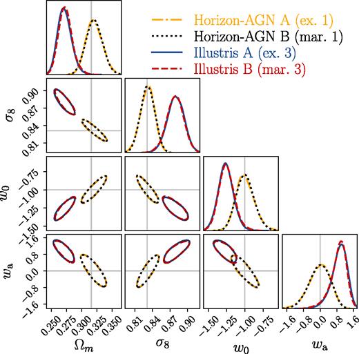
Comparison of the posterior distributions of cosmological parameters between baryonic physics mitigation techniques A and B listed in Table 3. The yellow dot–dashed and black dotted contours indicate the 1σ contours of the posterior probability distributions obtained from methods A and B, respectively, for the Horizon-AGN simulation after excluding or marginalizing over the first PC modes. Similarly, the blue solid and red dashed contours indicate the case for Illustris after excluding or marginalizing over three PC modes. The excellent match between the posterior probability distributions for cosmological parameters between methods A and B confirms that the PC exclusion formula shown in equation (13) is conceptually equivalent to marginalizing over PC amplitudes.
In conclusion, we have demonstrated with examples that the PC exclusion formula shown in equation (13) gives consistent results as when marginalizing over PC amplitudes with an uninformative prior. Method B can provide baryonic information through the constrained PC amplitudes, which can be used as a standard to quantify baryonic effects. So far, we allow the PC amplitudes to vary from (−∞, ∞). Reducing the prior ranges on PC amplitudes could potentially increase the constraining power on cosmology if we can develop a consistent way of setting the priors on PC amplitudes, given our knowledge of baryonic physics. The downside of method B is that it requires running longer MCMC chains to ensure convergence due to an increase in the dimensionality of parameter space. Therefore if one does not care to learn about baryonic physics, and would simply like to marginalize over it, we recommend method A.
5.2 Comparison between various PC construction methods
Here we compare the performances of the PCA-based methods listed Table 3. We have already shown in Section 5.1 that PC mode exclusion (method A) is equivalent to marginalizing over PC amplitudes (method B), so here we only compare methods A, C, and D.
The fundamental difference between these PCA methods is the way the PCs are constructed from the training simulations, which affects their efficiency in describing how baryonic physics modifies the data vectors on larger or smaller scales. We refer readers back to Section 4 for more details about this formalism. Briefly, when PCs are derived from |$\boldsymbol \Delta$| (method A; equation 8), they are most efficient in describing the difference vector |$\boldsymbol D-\boldsymbol M$|. For PCs trained from |$\boldsymbol \Delta _{\rm chy}$| (method C; equation 20), they are most efficient in describing the noise-weighted difference, |$\boldsymbol D_{\rm chy}-\boldsymbol M_{\rm chy} = \mathbf {L}^{-1}(\boldsymbol D-\boldsymbol M)$|, due to baryonic physics. Finally, PCs trained from |$\boldsymbol R$| (method D; equation 25) are most efficient in describing variations in the fractional difference |$\frac{\boldsymbol D-\boldsymbol M}{\boldsymbol M}$| from baryonic effects.
Fig. 9 shows the median of the marginalized 1D posteriors of cosmological parameters under different baryonic physics mitigation techniques for data vectors derived from our four test simulations. The lower and upper error bars represent for the 16th and 84th quantiles of the 1D marginalized posterior distribution. The x-axes indicate numbers of PC modes excluded or numbers of marginalization parameters used in the analysis. We select some cases from Fig. 9 and present their 1D and 2D posteriors in Fig. 10. The brown crosses in Fig. 9 indicate the case when no baryonic physics mitigation scheme is applied. One can see that the deviation from the fiducial cosmological parameters exceeds 1σ for all of our test baryonic scenarios. This is also shown in Fig. 4 on the 2D posterior contours. The blue-circle, red-triangle, and yellow-square markers indicate the results of performing baryonic physics mitigation by PCA-based methods A, C, and D, respectively. When the modifications of the data vectors due to baryonic physics are relatively weak as in MB2/Eagle/Horizon-AGN, we find that removing up to two PC modes is sufficient to marginalize baryonic bias to within 1σ10 for the cosmological parameters presented here. For the Illustris simulation, due to its strong baryonic feedback, we need to remove up to six PCs for the 1σ posteriors to include the fiducial cosmological parameters.
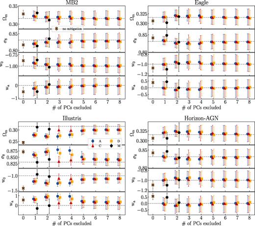
Marginalized 1D constraints on cosmological parameters when using different baryonic physics mitigation techniques from Table 3. Each panel is for a different input data vector based on a different hydrodynamical simulation as explained in the plot title. The grey dashed horizontal lines indicate the fiducial cosmological values. The marker position, the lower and upper error bars indicate the median, the 16th and the 84th percentiles of marginalized 1D posteriors. The brown crosses indicate the results when fitting the data vectors with the DMO-based emulator (halofit) without applying any baryonic physics mitigation technique. The blue circles, red triangles and yellow squares show the results when applying PCA-based methods A, C, and D, respectively, with their positions in the x-direction indicating how many PC modes are excluded or numbers of marginalization parameters used when doing the analysis. The black pentagons located at x = 1 indicate the result when only marginalizing over A in hmcode (with η0 fixed via equation 28). The black pentagons located at x = 2 are the results when marginalizing over both A and η0 in hmcode. For PCA-based methods, we find that the 1σ posteriors start to enclose the fiducial cosmology after removing two PC modes for MB2/Eagle/Horizon-AGN, while excluding six PC modes is required for more extreme baryonic scenarios of Illustris. When using hmcode to perform marginalization, except for the Illustris simulation for which marginalizing over A alone is enough, generally it is required to vary both A and η0 to mitigate baryonic effects to within 1σ.
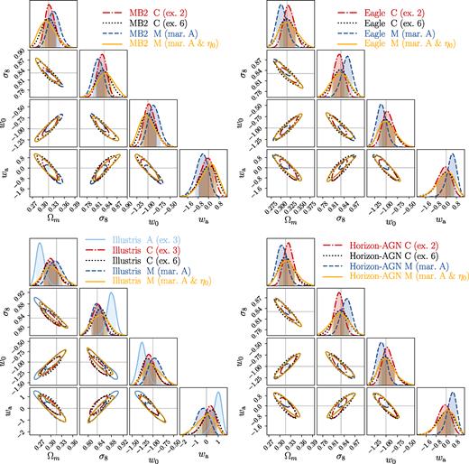
The 2D posterior distributions on cosmological parameters for some selected cases shown in Fig. 9. Each panel is for a different input data vector based on a different baryonic physics scenario as labelled in the legend. The legend also describes which baryonic mitigation techniques are applied, and how many PC modes are excluded or the hmcode parameters marginalized over.
5.2.1 Method C is superior to methods A and D
In Fig. 11 we plot the w0 bias (in colour-filled markers; defined as |w0,best fit − w0,fid|, with w0,best fit being the median value of the marginalized posterior distribution of w0) and the 0.5σ error of w0 (in open markers; with σ defined as the half difference between the 16th and 84th percentile of the 1D marginalized posterior of w0) for various baryonic physics mitigation schemes. For a method to be effective in mitigating baryonic-induced parameter biases, we require that the bias be below the 0.5σ errors. For all baryonic physics scenarios, we observe that at fixed number of excluded PC modes, the biases of method C (red-filled triangles) are nearly always smaller than methods A (blue-filled circles) and D (yellow-filled squares). If focusing on the lower left panel of Fig. 10, using Illustris when removing three PC modes as an examples, one can see that the 2D 1σ posteriors of method C (red dot–dashed curves) enclose the fiducial cosmology, while the posteriors of method A (light blue solid curves) are several σ away. Based on these, we conclude that PCs build from |$\boldsymbol \Delta _{\rm chy}$| are potentially more effective than others to mitigate baryonic effects.
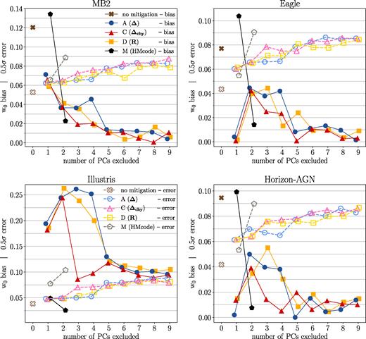
The w0 bias and statistical uncertainty under various baryonic physics mitigation techniques listed in Table 3. The darker coloured-filled markers indicate the level of w0 bias, defined as |w0,best fit − w0,fid|. The fainter unfilled markers indicate the 0.5σ statistical uncertainty, with 1σ defined as the half difference between the 16th and 84th quantiles of the marginalized 1D w0 posterior distribution. We adopt a criterion of residual bias <0.5σ error in this work when determining how many PC modes are required to mitigate biases due to baryonic physics. The four main lessons from this plot are that: (i) Of various PCA methods, at fixed number of excluded PC modes, the biases of method C are nearly always smaller than methods A and D, indicating method C is the most efficient PCA method. (ii) For MB2/Eagle/Horizon-AGN simulations, removing ≥2 PC modes is enough to mitigate baryonic physics-induced bias to 0.5σ. For the Illustris simulation, all PCA methods fail to pass the bias <0.5σ criteria even after nine PC modes are removed. (iii) No matter which PCA method (A, C, or D) is applied, after removing ≥6 PC modes, the statistical errors on w0 converge to similar values. (iv) hmcode works particularity well for the Illustris simulation. For MB2/Eagle/Horizon-AGN, marginalizing over both A and η0 is required to safely mitigate baryons to 0.5σ.
To understand why method C performs better, we can go back to the χ2 equation when both |$\boldsymbol D$| and |$\boldsymbol M$| are set at |$\boldsymbol p_{\rm co, fid}$|:

|$\left\langle \chi _{\rm bary}^2 \right\rangle$| quantifies the amount of χ2 caused by baryonic uncertainties. The noise term in our likelihood simulation is zero by construction. Our goal is to reduce |$\left\langle \chi _{\rm bary}^2 \right\rangle$| to avoid bias in cosmological parameters due to baryonic physics. From equation (29), one can see that when doing PC mode exclusion in |$\boldsymbol D_{\rm ch}-\boldsymbol M_{\rm ch}$| (with PCs constructed in |$\boldsymbol \Delta _{\rm chy}$|), there is a direct connection in reducing |$\left\langle \chi _{\rm bary}^2 \right\rangle$|, while when doing PC mode exclusion in |$\boldsymbol D-\boldsymbol M$| (with PCs constructed in |$\boldsymbol \Delta$|), the covariance matrix in between makes the reduction of baryonic uncertainties less direct.
5.2.2 Error bars converge for all PCA methods
Going back to Fig. 11, and focusing on the trend in the 0.5σ error bars of w0 shown in open fainter coloured markers. Generally, error bars grow as more PC modes are excluded (see also Fig. 10 for the growth of error ellipse on 2D posteriors). The size of the error bars varies among the different PCA methods when fewer PC modes are excluded, but eventually converges/saturates to similar error bar sizes when excluding ≳6 PC modes, independent of how PCs are constructed. This means that the PCs fully absorb the range of matter power spectrum modifications due to baryonic physics across the nine OWLS simulation, characterizing them using six dominant degrees of freedom; the last three PC modes are subjected to very small singular values (σ as depicted in Fig. 5) such that only a tiny amount of baryonic fluctuation would be projected on them. In principle, including more training samples with different features would enrich the PC pool, increasing the number of effective degrees of freedom to characterize other possible baryonic scenarios.
5.3 PCA framework versus hmcode
We now move to a more detailed comparison of the two main ways to marginalize over baryonic uncertainties, namely the PCA-based methods and the halo-model-based approach. Since we already compared in Section 5.2 that of all PCA methods listed in Table 3, method C is more efficient than the other two in mitigating biases in cosmological parameters due to baryonic physics. In the following, we will use method C as a representative for PCA-based methods, and compare it with hmcode (method M).
5.3.1 Comparison on the effectiveness (criterion: bias <0.5σ)
We begin by discussing the performance of hmcode when using only one (A) versus two (both A and η0) parameters to marginalize over baryonic physics. When only the parameter A is used, hmcode sets the η0 value via equation (28). Going back to Fig. 11, with w0 as an example, the pentagons at an x-axis value of 1 indicate the bias (black-filled) and 0.5σ error (grey-open) of only varying A in hmcode. Similarly, the pentagons at an x-axis value of 2 indicate the option for hmcode varying both A and η0. For the Illustris simulation, both options can successfully mitigate the baryonic bias on w0 to within our 0.5σ criterion. However, apart from Illustris, for the baryonic scenarios of MB2, Eagle, and Horizon-AGN, we find that varying only A while setting η0 following equation (28) is not sufficient to mitigate baryonic bias. This implies that the current empirical relation described in equation (28) may not be precise enough for MB2/Eagle/Horizon-AGN-like data vectors with LSST-like statistical power. We therefore recommend that the extra freedom carried by η0 is needed for upcoming weak lensing surveys to effectively mitigate the impact of baryonic physics on cosmological weak lensing measurements. This is even more true in light of recent findings that indicate that our Universe is not like Illustris, for which the AGN feedback is known to be too strong such that the baryon fractions in massive haloes are too low compared with observations (Haider et al. 2016). In Fig. D1 of Appendix D, we also provide similar bias and error plots for other cosmological parameters: Ωm, σ8, and wa. The same conclusion holds for HMcode on these cosmological parameters (as shown in the filled and open pentagons), except for the wa constraint for Illustris (Fig. D1 l), where varying only A is not enough to mitigate wa bias to within 0.5σ.
For the PCA-based method C, as indicated in red triangles of Fig. 11 for w0 and Fig. D1 for Ωm, σ8, and wa, we find that removing ≥3 PC modes is sufficient to mitigate baryonic uncertainties to within 0.5σ for all cosmological parameters considered here, if our Universe has a baryonic physics scenarios like MB2/Eagle/Horizon-AGN.
For the case of the Illustris simulation, we find that the PCA method fails to mitigate baryonic biases to within 0.5σ for w0 and Ωm (Fig. D1d), even after nine PC modes are removed, but just passes the threshold for σ8 (Fig. D1h) and wa (Fig. D1 l) after removing seven PC modes. We note that this is likely not a major concern as the baryonic effects of Illustris are unrealistically large, and the next-generation IllustrisTNG hydrodynamical simulation (Pillepich et al. 2018; Springel et al. 2018) will address the defects of the old version.
We provide a summary of the results from the above discussion in Table 4. In Appendix E, we further provide the χ2 values computed at the best-fitted cosmological parameters from various baryon mitigation models.
Summary of the effectiveness of baryonic physics mitigation methods in reducing biases to within 0.5σ for various cosmological parameters under different baryonic scenarios. A cosmological parameter is struck out if a mitigation method fails to pass our criterion of bias <0.5σ, where σ represents the marginalized statistical error (see Section 5.3.1 for detail).
 |
|
Summary of the effectiveness of baryonic physics mitigation methods in reducing biases to within 0.5σ for various cosmological parameters under different baryonic scenarios. A cosmological parameter is struck out if a mitigation method fails to pass our criterion of bias <0.5σ, where σ represents the marginalized statistical error (see Section 5.3.1 for detail).
|
|
5.3.2 Comparison on the level of degradation on cosmology
We now compare the error bars on cosmological parameter constraints between PCA method C and hmcode, on baryonic scenarios of MB2/Eagle/Horizon-AGN, where both methods successfully mitigate the baryonic biases to within 0.5σ. The pink open triangles in Fig. 11 indicate the 0.5σ error of w0 under method C, and the grey open pentagons indicate the same for hmcode. Besides w0, other cosmological parameters are also shown in Fig. D1. As discussed in Section 5.2.2, one nice feature of the PCA method is that the error bars converge to a certain level when excluding ≥6 PC modes. We find that the converged error bars for method C generally are smaller than those for hmcode, even though hmcode only utilizes two parameters to marginalize over baryonic physics uncertainties while the PCA method needs three parameters to mitigate baryonic effects to 0.5σ in the case of MB2/Eagle/Horizon-AGN. A similar result can be seen from the 1σ 2D posteriors shown in Fig. 10.
5.3.3 Baryonic feature constraint from hmcode
In Fig. 12, we plot the 2D posterior distributions on A and η0 for various baryonic scenarios in coloured contours, along with equation (28) shown in the black line. We can see that although relying on this A–η0 relationship is not effective enough to mitigate baryonic bias in most of baryonic recipes under LSST-like survey, the suggested relationship is still good enough to pass the 68 per cent contours in all cases. Therefore, instead of following a fixed relationship like equation (28) or allowing both A and η0 to vary unboundedly, setting an A-dependent prior on η0 may help recover some cosmological constraining power while still reducing biases in cosmological parameters when using hmcode.
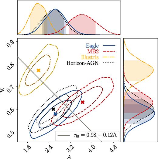
The 2D constraints on the hmcode halo structure parameters A and η0 from our simulated likelihood analysis for baryonic scenarios of Eagle (blue/solid), MB2 (red/dotted), Illustris (green/dot–dashed), and Horizon-AGN (yellow/dashed). The black line plots the relationship between A and η0 that is used to provide single-parameter fit in hmcode. Both 68 per cent and 95 per cent confidence levels are shown.
In Fig. 13, we compare the power spectra generated from hmcode at the best-fitted values of A, η0 (cross symbols in Fig. 12) to the original power spectra derived directly from the hydrodynamical simulations at redshift z = 0, 1, 2, 3. We note that this is not a fair comparison because the underlying Pδ(k, z) is not constrainable from the projected tomographic power spectra, unless the tomographic bins are fine enough to recover the full 3D information.11 Here we simply use these plots to understand the effects of hmcode parameters on Pδ(k, z). First, hmcode does not have degrees of freedom for the cooling feature of hydro simulations, which leads to a turn-over in the power spectrum ratio at |$k \gtrsim 10 \ h^{-1}\, \mathrm{Mpc}$|. This is expected as according to M15, the halo-model power is accurate to ≈5 per cent only for |$k \le 10 \ h^{-1}\, \mathrm{Mpc}$| and z ≤ 2. Because of this limitation, hmcode tends to produce a shallower suppression of power for a given k (when |$k \le 10 \ h^{-1}\, \mathrm{Mpc}$|) compared with MB2/Eagle/Horizon-AGN, in order to compensate for the lack of cooling prescription at |$k \gt 10 \ h^{-1}\, \mathrm{Mpc}$|. Secondly, the redshift evolution of hmcode power spectra is too monotonic, lacking freedom to capture the complicated evolutionary pattern that generally exists in hydrodynamical simulations. The redshift evolution patterns can be very different for various baryonic scenarios. hmcode’s inability to model redshift evolution may be due to the fact that only two nuisance parameters are involved in describing the complex scale and redshift dependences of baryonic effects seen in the simulations. One straightforward suggestions is to add redshift dependence to A and η0. Further development of halo model approaches to account for the modification of the matter power spectrum for |$k \gt 10 \ h^{-1}\, \mathrm{Mpc}$| is also needed. Although the current model does not describe all the complexity of possible modifications of P(k) due to baryonic physics, we can still use hmcode to gain insight into the strength of feedback from the constrained values of A and η0. As shown in Fig. 12, the Illustris-like universe tends to have small A and large η0.
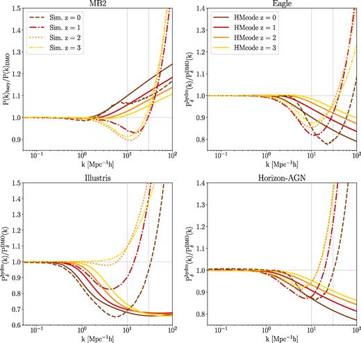
Comparisons of power spectra generated from hmcode at the best-fitting A and η0 values (solid lines) and power spectra directly derived from hydrodynamical simulations (dotted or dashed lines) at z = 0, 1, 2, 3. The discrepancy indicates that hmcode lacks degrees of freedom to account for the cooling effect at high k, and that it is too simplified to capture the complex redshift evolution patterns present in hydrodynamical simulations.
5.4 Pushing to even smaller angular scales: ℓmax of 5000
Until now, all elements of our analysis have been based on mock tomographic shear data vectors with ℓmax ≈ 2000, which is a conservative choice under the limitation that we lack accurate power spectra at |$k \gt 30 \ h^{-1}\, \mathrm{Mpc}$|. The ℓmax ≈ 2000 cut assures that various extrapolation curves on Pδ(k) ratio out to |$k \gt 30 \ h^{-1}\, \mathrm{Mpc}$| would not cause significant change on the resulting Cij(ℓ) data vector (see Appendix B for details on how the scale cut limit is determined).
To further test the limits of the proposed baryonic mitigation techniques, we generate mock Cij(ℓ) data vectors with ℓmax ≈ 5000 (based on the quadratic extrapolation trends derived by fitting the Pδ(k) ratio in |$k \in [10, 30] \ h^{-1}\, \mathrm{Mpc}$|, see the red curve in Fig. B1 as a demonstration), and then perform the same simulated likelihood analyses with mitigation techniques described in Sections 3 and 4. The only difference is that we append three extra data points that with equal logarithmic spacing in ℓ ∈ [2060, 5000] to the original data vector |$\boldsymbol D$| in each tomographic bin. The new length of |$\boldsymbol D$| is thus extended to 55 × (18 + 3) = 1155 data points (see Section 3.2 for the original format of |$\boldsymbol D$|). The covariance matrix is also updated accordingly.
The dark grey contours in Fig. 14 indicate the 2D posterior distributions of the cosmological parameters, when no baryonic physics mitigation technique is applied. Compared with the similar plot shown in Fig. 4, but for ℓmax ≈ 2000, the biases on cosmological parameters increases to 2σ–19σ for the various cosmological parameters in an Illustris-like universe, and around 1.5σ–6σ for the other cases. This amount of bias is consistent with fig. 5 of E15, who showed the posterior distributions for ℓmax ∼ 5000 for the OWLS baryonic physics scenarios for an LSST-like likelihood simulations.
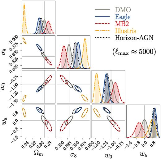
Similar to Fig. 4, but for the cases when pushing our mock observables towards ℓmax ≈ 5000.
Since we showed in Section 5.2 that method C is the most efficient of the PCA-based methods, we only run simulated likelihood analyses with PCA-based method C, compared with method M using hmcode for ℓmax ≈ 5000. In Fig. 15, we plot the marginalized w0 bias (colour-filled symbols) and 0.5σ w0 uncertainty (open symbols) as a function of the number of excluded PC modes in method C (blue diamonds) and hmcode (yellow hexagons). (The red triangles and black pentagons are simply copies of the data points shown in Fig. 11, to enable easier comparison of results with ℓmax of 2000 versus 5000.) The bias and error plots for Ωm, σ8, and wa are also provided in Fig. D1.

The w0 bias and uncertainty for the baryonic physics mitigation methods C (as our representative for PCA-based method) and M (halo model-based method/hmcode) (see Table 3 for details). The darker coloured-filled markers indicate the level of w0 bias, defined as |w0,best fit − w0,fid|. The fainter coloured-open markers indicate the 0.5σ w0 uncertainty, with 1σ defined as the half difference between the 16th and 84th percentile of the marginalized 1D w0 posterior distribution. The four key results on this plot are (i) the PCA method (blue diamonds) mitigates bias to within 0.5σ for the milder baryonic physics scenarios – MB2, Eagle, and Horizon-AGN – after excluding more than three PC modes, but fails for the Illustris scenario. (ii) When marginalizing over both A and η0, hmcode(yellow hexagons) mitigates w0 to within 0.5σ for all baryonic scenarios. (iii) For baryonic scenarios of MB2 and Eagle, the cases for which both methods work, the error bars for the PCA method (light blue open diamonds) converge to smaller values compared with hmcode(yellow open hexagons). (iv) Including more small-scale data in the analysis reduces the statistical error to |$\sim 20{{\ \rm per\ cent}}$| for PCA method (light blue open diamonds versus pink open triangles) and to about |$12\!-\!30{{\ \rm per\ cent}}$| for hmcode (yellow open hexagons versus grey open pentagons). (v) Including more training simulations in PCA improves reducing the w0 bias induced by neglecting baryonic effects to |$\sim 15{{\ \rm per\ cent}}$| for the case of Illustris (brown filled stars versus blue filled diamonds), although the improvement on residual bias is not reaching our criterion of <0.5σ.
Similar to Section 5.3, we rely on the bias <0.5σ criterion to validate the effectiveness of baryonic physics mitigation methods, with the results summarized in Table 5. First of all, for hmcode, varying only A is not sufficient to mitigate the bias to within 0.5σ for the Illustris simulation, which hmcode is particularly good at describing. Both A and η0 must be varied to meet our criterion for MB2 and Eagle. For Horizon-AGN and Illustris, hmcode works well for some cosmological parameters, while it fails for the others. For the PCA method, it still works for baryonic scenarios of MB2/Eagle/Horizon-AGN when pushing to ℓmax ≈ 5000, but continues to fail to meet our criterion for the Illustris scenario.
Similar to Table 4, but now for the likelihood simulations with mock observables pushing to ℓmax ≈ 5000.
 |
|
Similar to Table 4, but now for the likelihood simulations with mock observables pushing to ℓmax ≈ 5000.
|
|
In terms of degradation on cosmological parameter constraints after marginalization, for the cases of MB2 and Eagle, the scenarios in which both PCA and hmcode succeed in mitigating the bias to within 0.5σ, we see that PCA method yields smaller converged error bars (light blue open diamonds) compared with hmcode using two parameters (yellow open hexagons) to do marginalization.
Does extending the data vectors to ℓmax ≈ 5000 help to better constrain cosmological parameters compared with ℓmax ≈ 2000? As shown in Fig. 11, for the PCA method, we observe that the converged w0 errors for the ℓmax ≈ 5000 cases (light blue open diamonds) are smaller by |$\sim 20{{\ \rm per\ cent}}$| compared with the errors for ℓmax ≈ 2000 (pink open triangles). For the cases of hmcode when varying both A and η0, the w0 errors reduce by |$\sim 12{{\ \rm per\ cent}}$| for MB2, |$\sim 18{{\ \rm per\ cent}}$| for Eagle, and |$\sim 30{{\ \rm per\ cent}}$| for Horizon-AGN, after extending data points to ℓmax ≈ 5000 (yellow open hexagons) from ℓmax ≈ 2000 (grey open pentagons). This means that we do benefit from additional constraining power when including more small-scale data in the analysis, if the baryonic physics effect in our Universe is near the physics implemented in Eagle/MB2/Horizon-AGN.
5.5 Including more AGN prescriptions in the training set
The reason why the PCA method fails to mitigate the impact of baryonic physics on the matter power spectrum in Illustris is that the PCs built from the current training set do not capture the strong variation with k to explain its intense feedback feature. As also discussed in Mohammed & Gnedin (2018), it is better to have a training set that comprises adequately exotic but reasonable models. Of the nine training OWLS simulations, only the OWLS-AGN contains an AGN feedback prescription, and we rely on this single AGN model to explain Illustris. However, this shortcoming can be fixed by incorporating more training simulations into the PCA, so that the resulting PCs will include more degrees of freedom to explain the broader range of outcomes due to baryonic physics.
We try to address the above Illustris problem by including the baryonic scenarios of MB2/Eagle/Horizon-AGN in our training set, and then build a |${\boldsymbol \Delta _{\rm ch}}$| matrix with 12 columns to extend the capability of the derived PCs. In the bottom left panel of Fig. 15, we plot the marginalized w0 bias (brown filled stars) and error (light brown open stars) for Illustris simulation with PCs trained from the 12 baryonic scenarios, and a scale cut at ℓmax ≈ 5000. (The results for other cosmological parameters can be found in the last column of Fig. D1 as well.) With this expanded training set, the PCA method now reduces the w0 bias from 1.5σ (blue filled diamonds) to 0.8σ (brown filled stars), which is an improvement but still does not enable us to meet our criterion of bias <0.5σ.
The error bars when using 12 simulations in the training set converge after removing ≥6 PC modes. Notice that the converged errors become bigger when the PCs are trained from 12 simulations rather than just the 9 OWLS simulations. By including more simulations to construct the PCs, we also enlarge the range of baryonic uncertainties, which is a trade-off to ensure a more effective removal of biases due to baryonic physics for a broad range of baryonic physics scenarios. However, we can also imagine trying to rely on external information from independent observations to rule out baryonic scenarios that fail to describe our Universe. By carefully controlling the uncertainty range of the training set, we could potentially improve the cosmological constraining power after mitigation.
6 SUMMARY AND DISCUSSION
We have explored the two major approaches to mitigate uncertainties in cosmic shear tomographic power spectra due to baryonic physics, with the goal of understanding their performance on cosmological constraints for the upcoming LSST survey. The first approach is the PCA-based analysis proposed by E15. Based on a set of training hydrodynamical simulations with various baryonic prescriptions (spanned by OWLS in this work), a difference matrix (equation 8) is computed. Its columns are filled with difference vectors between these hydro and DMO simulations. PCA is then performed on the difference matrix to find dominant PC modes that can be used to model baryonic effects in other hydro simulations. The second approach is the halo model-based method coded in the package of hmcode by M15, which utilizes two halo structural parameters (A and η0) related to the halo concentration–mass relation to marginalize over baryonic uncertainties.
We examine the basics of the PCA formalism and provide a modification to properly account for the change of covariance matrix after removal of PC modes. Under the new formalism, we demonstrate that PC mode removal is equivalent to marginalization over PC amplitudes (see Section 5.1). Instead of difference matrices, we also investigate PCA on other kinds of matrix forms with their columns filled with the fractional difference (equation 25) or noise-weighted difference vectors (equation 20) to quantify deviations in the matter power spectrum due to baryonic physics. The derived PC bases from different matrices vary in their efficiency in explaining baryon fluctuations at different angular scales. Difference matrix PCs can more effectively account for large-scale baryonic fluctuations, fractional difference matrix PCs are more effective at describing the small-scale fluctuations, and noise-weighted difference matrix PCs most effectively describe the scales at which the S/N is maximal. We find that performing PCA on the noise-weighted difference matrix, with the weighting factor derived via performing Cholesky decomposition on the covariance matrix (Section 4.2), is the most efficient way to mitigate the impact of baryonic physics on inferred cosmological parameters (Section 5.2). Therefore, for future application on real data, we recommend applying the noise-weighted PCA technique. It should be noted that except for method D, the current PCs are wiggling slightly in their directions at each MCMC step, when cosmology changes. If we would like to quantify baryon physics via PC amplitudes, we hope the constrained PC amplitudes are subjected to a fixed set of PCs. A more complete design of PCA algorithm therefore would be an iteration process. We will first use the current setting to find the best-fitted cosmology, and once the |$\boldsymbol p_{\rm co, best\ fit}$| is determined, we will fix PC basis at |$\boldsymbol p_{\rm co, best\ fit}$|, and constrain the posteriors of PC amplitudes subjected to this PC set.
We apply both the PCA and hmcode techniques on mock shear tomographic data vectors (Cij(ℓ)) with baryonic physics scenarios of MB2/Eagle/Illustris/Horizon-AGN. We test whether these mitigation techniques can reduce the bias in cosmological parameters induced by neglecting baryonic effects to within 0.5σ. With a scale cut at ℓmax ≈ 2000, and for milder baryonic physics scenarios like MB2/Eagle/Horizon-AGN, both methods succeed in mitigating the impact of baryonic effects on the inferred cosmological parameters. For the PCA method, we find that excluding 3 PC modes is sufficient to mitigate the bias to within 0.5σ for Ωm, σ8, w0, and wa. For hmcode, we find that it is safer to vary both A and η0 when performing marginalization, rather than varying only one of them and having the other follow the suggested relation in M15, at least at the level of LSST statistical power. For the Illustris scenario, only hmcode is sufficient to mitigate the bias to within 0.5σ. The PCA method fails to pass our criterion even after removing nine PC modes. With a more aggressive ℓmax of 5000, the PCA methods still work for MB2/Eagle/Horizon-AGN, but fail for Illustris. hmcode remains sufficient for MB2/Eagle after marginalizing over two parameters but only works partially on some of the cosmological parameters for Horizon-AGN and Illustris, as summarized in Table 5.
We found that hmcode is most effective at mitigating the impact of baryonic physics for a strong feedback scenario like Illustris, because HMcode is designed to describe the impact of baryonic physics on the matter power spectrum for k ≤ 10 h Mpc−1, where the main feature is the suppression of power due to feedback (Fig. 1). hmcode and halo model-based approaches in general have the advantage over PCA that they have cosmology dependence built in. Although the current version of hmcode lacks the complexity to fully describe various baryonic scenarios (Fig. 13), it provides a good summary of the level of feedback strength through two nuisance parameters (Fig. 12). Future improvements of the halo model to smaller scales of k ≥ 10 h Mpc−1, as well as adding parameters to allow additional freedom in the redshift evolution of baryonic physics effects, may constrain halo structural parameters and baryonic power spectra ratio curve together with cosmology. Exploring the prior ranges on halo model parameters also help to improve cosmological parameter constraint. For example, we can use the posterior constraints from realistic hydrodynamical simulations as shown in Fig. 12 to narrow down the allowed ranges of A and η0. Joint constraints from galaxy–galaxy lensing together with cosmic shear may also provide additional information from the data itself on the halo structure parameters (Zentner et al. 2008).
There are several advantages of the PCA method. First, it successfully mitigates quite general baryonic fluctuations and complex redshift evolution patterns, when collecting several representative training hydrodynamical simulations to conduct PCA. The complex baryonic behaviours as well as the redshift evolution would then be naturally absorbed in only a few dominant PC modes, and we can use the amplitudes of these PC modes to perform marginalization (or, equivalently, PC mode exclusion). Secondly, the PCA method efficiently accounts for baryonic uncertainties without losing too much cosmological constraining power. As discussed in Section 5.3.2, whenever both methods are successful in removing baryonic bias, the error bars are generally smaller for PCA methods compared with the errors of hmcode. It is quite important to note that even if we do not know in advance how many PC modes must be excluded to safely remove baryonic bias in our Universe, excluding all effective PC modes does not unacceptably increase the errors, which saturate at a certain limit. The maximum number of effective PC modes one can remove is equal to the total number of training simulations used in the PCA (see Section 4.1.1 for detail). Finally, the PCA method has significant flexibility to make adjustments as our knowledge of baryonic physics improves. For example, in Section 5.4 we tried to improve the bias mitigation of the Illustris simulation by including more realistic baryonic scenarios with AGN prescriptions in our training set, which enriches the space of possible baryonic uncertainties that the PCs can describe. After the inclusion of MB2/Eagle/Horizon-AGN as well as the original nine OWLS scenarios in our training set, we can further decrease the residual cosmological parameter bias compared with the results when only using the nine OWLS simulations as training set. The cost is that we lose some constraining power. The flexibility of the PCA framework makes it easy to adjust the model based on changes in our knowledge of baryonic physics, and allows us to regulate errors by controlling the input training simulations in the PCA.
There are several aspects regarding the PCA framework that we do not explore within this work. First, our training hydro simulations are all run under the flat ΛCDM model, and we assume that the baryonic fluctuations, as quantified in terms of power spectrum ratios between hydrodynamical and DMO simulations, remain fixed when cosmology changes. In reality, baryonic and cosmological effects vary jointly. Currently, there is no easy way to investigate this assumption, but future fast hydrodynamical simulations under development would be an ideal tool to systematically study this issue. Secondly, we adopted a power-law extrapolation scheme for Pδ(k) ratio at k ≥ 30 h Mpc−1 (see Appendix B). The most relevant physics that governs the high k behaviour is the cooling and inner stellar density profile of galaxies. Current large-volume cosmological hydrodynamical simulations lack the resolution to resolve the physics of galaxy formation to galaxy centres. We rely on subgrid models of feedback to avoid the overcooling of gas and to mitigate the differences between the observed and simulated galaxies, but discrepancies still exist (Stinson et al. 2010; Bottrell et al. 2017; Furlong et al. 2017). This implies that Pδ(k) in the high k regime is still highly uncertain. Does the Pδ(k) ratio continue the trend of increasing monotonically? Or should it reach a saturation point at some high k regime? How to properly propagate the uncertainties of the poorly understood small-scale Pδ(k) ratio into the errors of integrated Cij(ℓ) which in turn affects the derived PCs? These questions require higher resolution hydrodynamical simulations to further address. Finally, we have briefly demonstrated in Section 5.5 that depending on the training simulation set, the derived PCs carry different abilities to mitigate baryonic effects, and differ in the final constraining power. It would be worthwhile to systematically investigate various possible combinations of the training simulations, to find a most effective set of PCs that are able to span a wide enough range of baryonic uncertainties but with less degradation on constraining power.
In future extensions of this work, we will apply the PCA framework to a configuration-space tomographic shear analysis on real data to constrain the baryonic feature of our Universe and compare it with hydrodynamical simulations. We aim to develop a consistent way of quantifying priors of PC amplitudes, which would provide us with more constraining power on cosmological parameters by shrinking the allowed range of baryonic physics modifications of the matter power spectrum. We will also develop a PCA tool for joint analysis of galaxy–galaxy lensing and galaxy clustering observables. The full 3 × 2-point analysis then can be self-consistently analysed within the PCA framework to increase the constraining power on cosmology while safely marginalizing over baryonic physics.
ACKNOWLEDGEMENTS
We thank Alex Hall for reviewing this paper and providing useful suggestions to improve the manuscript. We thank Sukhdeep Singh, François Lanusse, Qirong Zhu, Arya Farahi, Hy Trac, Phil Bull, Tiziana Di Matteo, Alexander Mead, Irshad Mohammed, and Ananth Tenneti for many constructive discussions and feedback. RM and HH are supported by the Department of Energy Cosmic Frontier program, grant DE-SC0010118. Part of the research was carried out at the Jet Propulsion Laboratory, California Institute of Technology, under a contract with the National Aeronautics and Space Administration and is supported by NASA ROSES ATP 16-ATP16-0084 grant.
Footnotes
Due to the low resolution of BAHAMAS, we are not able to include it as one of the hydrodynamical scenarios in this work (see Appendix B2 for details of our resolution requirement).
Although we plot |$\boldsymbol D_{\rm ch} - \boldsymbol M_{\rm ch}$| versus ℓ in Fig. 7, we note that actually the new data points are not strictly functions of the original ℓ because of the non-zero off-diagonal terms in |$\mathbf {L}^{-1}$|. However, our take-away point from Fig. 7 still holds due to the fact that our covariance matrix is dominated by Gaussian noise, and thus the off-diagonal terms in |$\mathbf {L}^{-1}$| are small.
The 1σ criterion is a looser condition than the 0.5σ constraint we will later use for defining acceptability; we use this looser condition here as we are just trying to compare the basic behaviour of the different PCA methods here. Once we are comparing the best-performing PCA methods with hmcode, we will consistently impose a 0.5σ constraint on both.
If using hmcode to directly fit the 3D matter power spectrum including baryonic effects at some specific redshift, according to M15, by adjusting A(z), and η0(z), hmcode has enough degrees of freedom to match the baryonic power spectra from the OWLS simulations to |$k \gtrsim 10 \ h^{-1}\, \mathrm{Mpc}$|.
Chisari et al. (2018) have estimated the effect of cosmic variance on the power spectrum ratio (see their fig. 5) by subsampling the Horizon-AGN simulation with a volume that is eight times smaller than our setting here. So the expected 1σ error due to cosmic variance in their case should be on the order of 1 per cent (|$\sqrt{8}$| times larger than our setting). The total spread of their subsampled power spectra ratios is consistent with our derivation within 3σ.
We refer readers to this link for more detail about Chi-square difference test.
REFERENCES
APPENDIX A: POWER SPECTRUM COMPUTATION
Here we describe the practical implementation of our power spectrum computation from the simulation snapshots.
A1 The power spectrum estimator
A2 The accuracy of power spectrum
For hydrodynamical simulations, the convergence properties are more difficult to systematically quantify due to the interplay between resolution effects and galaxy formation physics. For example, as the resolution increases, more lower mass haloes are resolved, leading to an increased power of SN feedback. Subgrid parameters regulating SN feedback then must be modified to account for this effect in order to match the observables like galaxy stellar mass function. Typically subgrid prescriptions are designed to reach some level of convergence with the variation of resolution. However, the functionality of such self-regulation is rather limited. Eagle is currently the only hydro simulation with its subgrid model parameters re-calibrated to match observations when the resolution is changed (see fig. 7 of Schaye et al. 2015). In the left-hand panel of fig. A2 in van Daalen et al. (2011), they showed a convergence comparison between the power spectra of OWLS-REF hydro simulations with kNy of 16 (the current OWLS resolution used in this work) and 32, respectively. The two baryonic power spectra agree to within |$\sim 10{{\ \rm per\ cent}}$| out to k ≈ 40 h Mpc−1. We note that this statement only applies to OWLS-REF. There is no general rule on the behaviour of convergence for hydro simulations, given that the galaxy observations are not yet converged, and that the subgrid prescriptions are all different.
APPENDIX B: POWER SPECTRUM RATIO
The power spectrum ratio between hydrodynamical and DMO simulations is an important quantity in this work. We rely on it in equation (1) to derive mock observables at different cosmology, as well as to build difference matrices to perform PCA. Here we discuss the validity of our estimates of this ratio over the range of scales used throughout this work, and describe how we perform extrapolation to smaller scales than those that are well-described in the simulation.
B1 Discussion on the convergence of the power spectrum ratio
The ratios of matter power spectra that we use in this work are accurate to k ≲ 30 h Mpc−1 for Eagle/MB2/Illustris/Horizon-AGN and of k ≲ 10 h Mpc−1 for OWLS. Below we will justify this claim.
The hydrodynamical and DMO runs are set at exactly the same initial conditions, and baryonic effects are negligible on large scales. When Pδ,hydro(k) ≈ Pδ,DMO(k) and Cov[Pδ,hydro(k), Pδ,DMO(k)] ≈ 1, as is the case at small k, we expect the variance of the power spectrum ratio in equation (B1) to approach zero.
On small scales, as discussed in Section A2, Pδ(k) would achieve |$1{{\ \rm per\ cent}}$| convergence out to k ≈ kNy/2. Hence, we expect the uncertainty in the power spectrum ratio due to limited simulation resolution to be |$\lt 2{{\ \rm per\ cent}}$| to k ≈ kNy/2, where kNy/2 is ∼30 h Mpc−1 for Eagle/MB2/Illustris/Horizon-AGN and ∼10 h Mpc−1 for OWLS.
If we naively derive the power spectrum ratio by using the raw data points of |$P_{\delta , \rm DMO}(k)$| and |$P_{\delta , \rm hydro}(k)$| at k > kNy/2, the derived ratio will be overestimated due to the underestimation of the denominator of |$P_{\delta , \rm DMO}(k)$| at scales of several times kNy, and underestimated towards even higher k due to the overestimation of |$P_{\delta , \rm DMO}(k)$| (see Section A2). We will introduce our extrapolation scheme below to avoid the biases.
B2 Power spectrum ratio extrapolation scheme
For scales below k < 0.1 h Mpc−1, we simply let the ratio curve asymptotically approach one, which is a justifiable assumption since we know that baryons hardly modify the matter power spectrum on large scales. For small scales, as shown in Fig. 1, the power spectrum ratio between hydrodynamical and DMO simulations tends to increase after k ≳ 20 h Mpc−1. This increase is caused by cooling effects in hydrodynamical simulation. In order to capture this physical effect, we make use of data points in k ∈ [10, 30] h Mpc−1, perform a smooth quadric spline fitting in |$\log (k) - \log (P_{\delta \rm , bary }(k) / P_{\delta \rm , DMO }(k))$| space, and extrapolating the fitted trend out to k > 30 h Mpc−1. Fig. 1 shows the extrapolation curves for all baryonic scenarios.
The above extrapolation scheme holds for Eagle/MB2/IIIustris/Horizon-AGN simulations, where we have reliable power spectrum ratios in the range k ∈ [10, 30] h Mpc−1. For the OWLS simulation set, as discussed above, the ratio data is only well-determined to k < 10 h Mpc−1. The black line in Fig. B1 indicates the naively derived power spectrum ratio from the raw data of OWLS-AGN and OWLS-DMO. In the case of OWLS-AGN, we do need data points slightly beyond k of 10 h Mpc−1 to capture the transition from suppression to enhancement of power. We therefore still make use of the raw data points in the range of k ∈ [10, 30] h Mpc−1, where the uncertainties may |$\gt 2{{\ \rm per\ cent}}$| but not that worse, to perform extrapolation spline line fitting, and the resulting curve is indicated in the red-dashed curve of Fig. B1. The raw data curve is slightly higher than the extrapolating curve when k is large. This is resulting from the underestimation of the DMO power spectrum as discussed in Section A2 and Section B. The extrapolation based on fitting data at k ∈ [10, 30] h Mpc−1 may exhibit uncertainties in the final extrapolation slope at high k. Therefore, we try to explore such uncertainties by setting slightly different extrapolating parameters that are shown as upper (yellow line) and lower (brown dot–dashed) bounds in Fig. B1. Finally, we also check the simplest constant extrapolation scheme as shown in the dark blue line. We will explore the effects of different extrapolation schemes on the resulting tomographic shear power spectra later.
![Power spectrum ratio between OWLS-AGN and OWLS-DMO at z = 0, assuming different extrapolation schemes above k > 10 h Mpc−1. The black line shows the raw data calculated by simply taking ratio from the raw OWLS power spectra from van Daalen et al. (2011). The red dashed line indicates the extrapolation scheme by extending a quadric spline fitted curve using the raw data points in k ∈ [10, 30] h Mpc−1. The yellow and brown dot–dashed lines indicate the two possible upper and lower bounds one may derive, if there is some uncertainty in the raw data points k ∈ [10, 30] h Mpc−1. The dark blue line plots a pure flat extrapolation. The light blue dash–dot–dotted line indicates the case of extrapolation when using data points in k ∈ [3, 10] h Mpc−1, which are believed to be well-measured.](https://oup.silverchair-cdn.com/oup/backfile/Content_public/Journal/mnras/488/2/10.1093_mnras_stz1714/2/m_stz1714figb1.jpeg?Expires=1750512172&Signature=V5L3rHdEICdl481YwaCL0dRWazaZi8FmeNIFvYBkYg7eeRss3LpCOrpbWvIx0dInzA2fU~fgTWD98uzJQytHSiHiSkhr8j16bPY6ZUK-kTSVuj~TILi1WxDWyLM9uymebfKwXWlHoW6QMqgujPLXxYb097~XT1I9094oy1uSn2ZEeuiDyOLVLefH5L-byKrFRkskfpZv2HpI9MsIadmPXfy31KcCSshI2VaXi341Gy3D0ihFZjdFZTp5cVCKXBPtrH7~BmNAASNwHgCVgxrl6bnagYeVT8b8h~MdECCvw056gQYA66g8KZAHmlT0NIwDIkH31x9ZBbMI-4PiFKVkbQ__&Key-Pair-Id=APKAIE5G5CRDK6RD3PGA)
Power spectrum ratio between OWLS-AGN and OWLS-DMO at z = 0, assuming different extrapolation schemes above k > 10 h Mpc−1. The black line shows the raw data calculated by simply taking ratio from the raw OWLS power spectra from van Daalen et al. (2011). The red dashed line indicates the extrapolation scheme by extending a quadric spline fitted curve using the raw data points in k ∈ [10, 30] h Mpc−1. The yellow and brown dot–dashed lines indicate the two possible upper and lower bounds one may derive, if there is some uncertainty in the raw data points k ∈ [10, 30] h Mpc−1. The dark blue line plots a pure flat extrapolation. The light blue dash–dot–dotted line indicates the case of extrapolation when using data points in k ∈ [3, 10] h Mpc−1, which are believed to be well-measured.
If only using data points around k < 10 h Mpc−1 to perform smooth extrapolation, one would fail to capture the cooling effect that typically exists in hydrodynamical simulations at high k. The light blue dash–dot–dotted line of Fig. B1 indicates such an extrapolation based on the data points for k ∈ [3, 10] h Mpc−1. This sets a very important requirement for our method. If we really want to use the PCA framework to achieve better cosmological parameter constraints by including more small scale information, the simulations that are used to build the PC basis must also have high enough resolution to construct a reasonable extrapolation down to the scale that goes into cosmological analysis. This is the reason why we avoid using the Rudd, Zentner & Kravtsov (2008) and Gnedin, Kravtsov & Rudd (2011) simulations to build our PC basis as in the previous work of E15. The half-Nyquist wavenumbers of these two simulations are too low to capture the up-turn in the power spectrum ratio, given the angular scales of ℓ ≈ 2000 used in this work.
We now justify how the choice of angular scale cut at ℓ ≈ 2000 is made. In Fig. B2 we present the computed tomographic shear power spectra in our lowest redshift bin, for various extrapolation schemes on the power spectra ratio shown in Fig. B1. The vertical grey line indicates the angular scale cut of ℓ = 2060 we have adopted. One can see that the Cij(ℓ) ratio only differs mildly at this scale. Therefore, although our current extrapolation scheme may lead to a considerable error in the Pδ(k) ratio, after the integration process, such error propagation in Cij(ℓ) ratio is estimated to be within 10 per cent when making an ℓ cut at ≈2000. We make a conservative choice of cutting in ℓ such that the final result is not too sensitive to our extrapolation scheme.
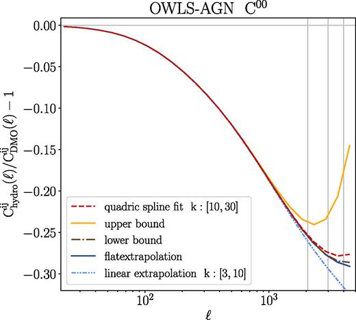
The ratio of tomographic shear power spectrum between OWLS-AGN and OWLS-DMO simulations for our lowest tomographic bin. Curves in different colours represent different Pδ(k) ratio extrapolation schemes as coloured in Fig. B1. The vertical dashed line indicates the angular scale of ℓ = 2060, where the cut is made for all of tomographic bins in our data vector. This cut is chosen such that the derived Cij(ℓ) curve would not be too sensitive on different Pδ(k) ratio extrapolation schemes.
APPENDIX C: COMPUTING BARYON-CONTAMINATED DATA VECTORS AT VARYING COSMOLOGY
In this appendix, we describe in detail how we compute baryon-contaminated data vectors as a function of cosmology. This procedure is needed to build the difference matrix (equation 8), weighted difference matrix (equation 20), or ratio matrix (equation 25) when doing PCA.
![The ratio of tomographic power spectra ratio at bin C00 between hydrodynamical and DMO simulations evaluated at various $\boldsymbol p_{\rm co}$ versus $\boldsymbol p_{\rm co, fid}$, i.e. ${}[\frac{C^{00}_{\rm hydro}(\boldsymbol p_{\rm co})}{C^{00}_{\rm DMO}(\boldsymbol p_{\rm co})}] / [\frac{C^{00}_{\rm hydro}(\boldsymbol p_{\rm co, fid})}{C^{00}_{\rm DMO}(\boldsymbol p_{\rm co, fid})}]$. Here different curves indicate changes of Ωm or σ8 to values shown in the legend, while keeping the remaining cosmological parameters the same as $\boldsymbol p_{\rm co, fid}$. The fact that all ratio curves are ≈1 to within 0.25 per cent indicates the validity of using equation (C2) as our approximation.](https://oup.silverchair-cdn.com/oup/backfile/Content_public/Journal/mnras/488/2/10.1093_mnras_stz1714/2/m_stz1714figc1.jpeg?Expires=1750512172&Signature=orZ588Mn60zoHE6RxmC-TRByuE75jhqoPUjitOjRmmXnbd1CAVQ0oumLNPr2C6Djmboe1ocdQ~hm4KxDCixWEJx5uioH-IFJIfmS4m9aijkyZw7ifKR7Mh6aN8NvAKKOXOJiAsQytr7xQxGA57udMOoSljcEnKP58Rv5ynIH0J-9vCCtiPN5Br08iVEnQCN3Nd-pa6ivskwVrgbAJH90Hhu9Bh114ecazBapmO4ZET-4SeSrpb6CZOGlRF-bFw-1VCO6qaUqd~qOi5zXiFlWPi~sNRPoOcrBwfTzOdbwTY-JjfRjoP9YYgjNowhOH70KFW2s5-2UiRt2fG4PSam2jg__&Key-Pair-Id=APKAIE5G5CRDK6RD3PGA)
The ratio of tomographic power spectra ratio at bin C00 between hydrodynamical and DMO simulations evaluated at various |$\boldsymbol p_{\rm co}$| versus |$\boldsymbol p_{\rm co, fid}$|, i.e. |${}[\frac{C^{00}_{\rm hydro}(\boldsymbol p_{\rm co})}{C^{00}_{\rm DMO}(\boldsymbol p_{\rm co})}] / [\frac{C^{00}_{\rm hydro}(\boldsymbol p_{\rm co, fid})}{C^{00}_{\rm DMO}(\boldsymbol p_{\rm co, fid})}]$|. Here different curves indicate changes of Ωm or σ8 to values shown in the legend, while keeping the remaining cosmological parameters the same as |$\boldsymbol p_{\rm co, fid}$|. The fact that all ratio curves are ≈1 to within 0.25 per cent indicates the validity of using equation (C2) as our approximation.
APPENDIX D: Constraints on cosmological parameters of Ωm, σ8, and wa
In this appendix, we provide constraints on cosmological parameters of Ωm, σ8, and wa after applying baryon mitigation techniques using hmcode or various PCA methods. The solid markers indicate the amount of residual bias after mitigation, and the open markers indicate the 0.5σ errors on the marginalized 1D posteriors. We rely on this plot to check whether a mitigation method can successfully reduce the baryonic physics-induced bias to within 0.5σ for different cosmological parameters and baryonic scenarios. The results are briefly summarized in Tables 4 and 5. We refer readers back to discussions at Sections 5.3 and 5.4 for details.
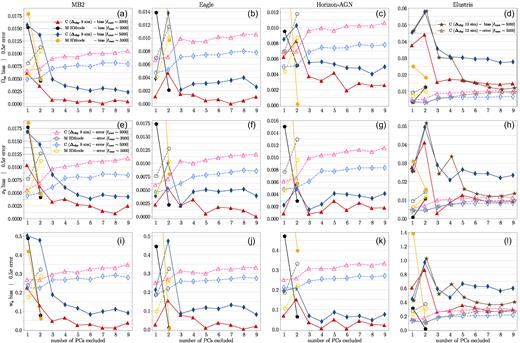
Similar to Fig. 15, but for cosmological parameters of Ωm (first row), σ8 (second row), and wa (third row), for various baryonic scenarios categorized in each different column.
APPENDIX E: GOODNESS OF FIT FOR BARYON MITIGATION MODELS
In this appendix, we summarize the fitting quality for various baryon mitigation methods. In Table E1, we provide the χ2 values computed at the best-fittng (fiducial) cosmology for hmcode and the PCA method C when applied on each baryonic scenario for the ℓmax ≈ 2000 likelihood simulations. Here we define our best-fitted parameters to be the median value at the marginalized 1D posterior distribution.
Goodness of fit for various baryon mitigation models.
| Eagle | MB2 | Horizon-AGN | Illustris | |
|---|---|---|---|---|
| No-mitigation at |$\boldsymbol p_{\rm co, bestfit}$| (|$\boldsymbol p_{\rm co, fid}$|) | 2.68 (30.92) | 0.93 (5.71) | 3.85 (103.2) | 107.5 (3258) |
| hmcode – A | 2.09 | 0.74 | 2.34 | 4.84 |
| hmcode – A, η0 | 0.91 | 0.29 | 1.69 | 4.80 |
| PCA ex1 at |$\boldsymbol p_{\rm co, bestfit}$| (|$\boldsymbol p_{\rm co, fid}$|) | 1.39 (3.25) | 0.70 (5.11) | 0.75 (6.75) | 11.91 (40.0) |
| PCA ex2 | 0.41 (0.39) | 0.37 (0.81) | 0.45 (2.72) | 9.68 (34.2) |
| PCA ex3 | 0.28 (0.24) | 0.28 (0.32) | 0.26 (2.65) | 3.08 (12.0) |
| PCA ex4 | 0.15 (0.07) | 0.18 (0.30) | 0.20 (1.38) | 2.06 (4.89) |
| PCA ex5 | 0.13 (0.04) | 0.14 (0.07) | 0.16 (0.64) | 1.65 (2.55) |
| PCA ex6 | 0.09 (0.03) | 0.11 (0.06) | 0.20 (0.59) | 1.58 (2.18) |
| PCA ex7 | 0.11 (0.03) | 0.12 (0.06) | 0.19 (0.54) | 1.50 (2.00) |
| PCA ex8 | 0.09 (0.03) | 0.08 (0.06) | 0.15 (0.53) | 1.44 (2.00) |
| PCA ex9 | 0.07 (0.03) | 0.10 (0.05) | 0.15 (0.43) | 1.37 (2.00) |
Notice that because our mock data vectors are noiseless, the χ2 values cannot be used to make statements about overfitting or underfitting based on the reduced χ2 criterion [i.e. we do not expect |$\chi ^2/\rm {(d.o.f.)} \approx 1$|]. However, using the information from the relative χ2 values (Δχ2) and the relative degrees of freedom (Δ d.o.f.) between two models, we can determine the model complexity needed from the data by performing the Chi-square difference test.13
For example, for the Illustris scenario, we see that when comparing the PCA results between excluding one PC mode to five PC modes, the Δχ2 = 11.91 − 1.646 = 10.264, and the Δ d.o.f. = 4. The corresponding p-value is 0.036, which means that the improvement is marginally statistically significant (p-value < 0.05). Excluding six PC modes does not significantly improve the goodness of fit compared with the result when excluding five PC modes (Δχ2 = 0.062, Δ d.o.f. =1, p-value =0.8).
After a few PC modes are excluded, we see that the χ2 values computed at |$\boldsymbol p_{\rm co, bestfit}$| is comparable to that computed at |$\boldsymbol p_{\rm co, fid}$| for all baryonic scenarios. This means that excluding PC modes does not just reduce parameter bias in our simulated likelihood analysis, but the resulting best-fitting model also provides a good fit to the data.
