


Abstract
The centre determination of a galaxy cluster from an optical cluster finding algorithm can be offset from theoretical prescriptions or N-body definitions of its host halo centre. These offsets impact the recovered cluster statistics, affecting both richness measurements and the weak lensing shear profile around the clusters. This paper models the centring performance of the redMaPPer cluster finding algorithm using archival X-ray observations of redMaPPer-selected clusters. Assuming the X-ray emission peaks as the fiducial halo centres, and through analysing their offsets to the redMaPPer centres, we find that |${\sim } 75\pm 8 {{\ \rm per\ cent}}$| of the redMaPPer clusters are well centred and the mis-centred offset follows a Gamma distribution in normalized, projected distance. These mis-centring offsets cause a systematic underestimation of cluster richness relative to the well-centred clusters, for which we propose a descriptive model. Our results enable the DES Y1 cluster cosmology analysis by characterizing the necessary corrections to both the weak lensing and richness abundance functions of the DES Y1 redMaPPer cluster catalogue.
1 INTRODUCTION
The abundance of galaxy clusters is a sensitive probe of cosmological models (see reviews and the referenced literature in Allen, Evrard & Mantz 2011; Weinberg et al. 2013). Cluster cosmology studies from the latest optical imaging surveys such as the Dark Energy Survey (the DES Collaboration, in preparation) will deliver significant improvement in precision over previous studies based on the Sloan Digital Sky Survey (SDSS, Rozo et al. 2010) and require (McClintock et al. 2019) accurate understanding of various systematic effects such as the orientation of clusters (Noh & Cohn 2012; Dietrich et al. 2014), correlated structures and their projection effect (Erickson, Cunha & Evrard 2011; Costanzi et al. 2019), mass profile modelling uncertainties (McClintock et al. 2019), and the contamination of cluster member galaxies in the lensing measurements (Varga et al. 2018).
One such important systematic effect is the mis-identification of cluster centres (Johnston et al. 2007a,b; Melchior et al. 2017; Simet et al. 2017; McClintock et al. 2019; the DES Collaboration, in preparation). Cluster observables, e.g. gravitational shear profiles, must be compared to models in order to derive constraints on parameters, and the models are based on some definition of cluster centre, described theoretically or on the basis of the matter density field in N-body simulations. Cluster lensing studies based on data from DES (McClintock et al. 2019) require accurate knowledge of cluster mis-centring fraction and offset distribution in order to forward model masses using analytic halo profiles.
Optical cluster finders often attempt to identify a central galaxy as the centre (Koester et al. 2007; Hao et al. 2010; Rykoff et al. 2014; Oguri et al. 2018). These central galaxies are typically quenched of star formation activities and may appear to be the brightest galaxy in a cluster (see studies in Skibba et al. 2011; Lauer et al. 2014; Hoshino et al. 2015). The identification of cluster central galaxies may seem straightforward given their dominant appearances, but mis-identifications or offsets relative to any other theoretical definition of centre is inevitable. Because massive haloes experience growth through mergers, cluster central galaxies can be displaced from the local gravitational potential minimum (e.g. Martel, Robichaud & Barai 2014). A related effect is when a second galaxy within the halo is chosen as the centre by the cluster finding algorithm. For a colour-based scheme focused on the reddest galaxies, this may happen if the central galaxy of the host halo has experienced recent star formation (e.g. McDonald et al. 2012; Donahue et al. 2015) or if a merging event brings in two nearly identical central galaxies of the progenitor haloes, as in the case of the Coma cluster (e.g. Vikhlinin et al. 2001). Another cause of mis-centring is when galaxies lying outside the primary host halo, but aligned in projection, are chosen as the central galaxy by the cluster finding algorithm.
The centring performance of optical cluster finding algorithms has been characterized with various methods. Cluster hot gas is an excellent tracer of the cluster potential as the dominant baryonic mass component. Cluster X-ray or thermal Sunyaev–Zel’dovich (tSZ) observation centres, identified as the centroids or the peaks of the surface brightness, are often used to calibrate the optically selected centres (see examples of X-ray studies in Lin & Mohr 2004; Stott et al. 2012; Mahdavi et al. 2013; Lauer et al. 2014; Rozo & Rykoff 2014; Rykoff et al. 2016; Zhang et al. 2016 and examples of tSZ studies in Song et al. 2012; Saro et al. 2015). Other than calibration to centres identified in multiwavelength observations, cluster centring has been characterized through comparing cluster radial profiles (lensing or galaxy number count) to those of a cluster sample with well-known centres from X-ray or optical data (Hikage et al. 2018; Luo et al. 2017) and through examining the velocity and separation distribution of cluster satellite galaxies (Skibba et al. 2011).
In this paper, we characterize the centring performance of the redMaPPer cluster finding algorithm – a method for identifying galaxy clusters from optical imaging data. The redMaPPer algorithm excels in producing a complete and efficient cluster sample with an accurate richness mass proxy and precise redshift estimations, as characterized with multiwavelength and spectroscopic data (Rykoff et al. 2012; Rozo & Rykoff 2014; Rozo et al. 2015a,b; Saro et al. 2015; Murata et al. 2018). Cluster catalogues constructed from SDSS (Rykoff et al. 2014) and DES data (Rykoff et al. 2016) are used to derive cosmological constraints in Costanzi et al. (2018) and the DES Collaboration (in preparation). In terms of the cluster centre identification, redMaPPer is not exempt from occasional mis-identification of the central galaxy.
The centring distribution of the redMaPPer algorithm has been studied using almost all of the aforementioned methods (Rozo & Rykoff 2014; Saro et al. 2015; Rykoff et al. 2016; Hikage et al. 2017). In this paper, we model the cluster centring distribution with 211 high-signal-to-noise X-ray cluster detections associated with the redMaPPer SDSS DR8 and DES Year 1 samples from the Chandra public archives, and the model constraints are then validated with X-ray cluster detections from the XMM public archives. We focus on the modelling aspects of redMaPPer centring performance in this paper, while the X-ray data processing procedures are presented in Hollowood et al. (2018) and Giles et al. (in preparation). The data set and methods we employ allow us to analyse the redMaPPer centring performance with the highest precision to date. We also develop a model to characterize how mis-centring affects redMaPPer richness estimation and discuss the impact of cluster mis-centring on cluster cosmology analyses. It is the first time that this effect has been quantified.
This paper is a companion paper to the DES and SDSS cluster weak lensing and cosmology studies presented in McClintock et al. (2019), Costanzi et al. (2018), and the DES Collaboration (in preparation). It uses similar data products to Farahi et al. (2019).
Throughout this paper, we assume a Flat Λ cold dark matter cosmology with h = 0.7 and Ωm = 0.3.
2 DATA
2.1 The redMaPPer catalogues
The redMapper algorithm examines galaxy colour, spatial overdensity, and galaxy luminosity distribution to identify possible galaxy clusters. Cluster centres are placed on a central galaxy candidate according to the colour, luminosity, and galaxy overdensity computed around the galaxy. Up to five central galaxy candidates are recorded for each cluster with probabilities assigned to them. The cluster centre is chosen to be the most probable one. The redMaPPer algorithm also estimates a richness as a mass proxy, λ, which is a probabilistic count of red sequence galaxies within an aperture centred on the central galaxy candidate. Detailed presentation of this algorithm can be found in Rykoff et al. (2014, 2016).
The redMaPPer samples studied in this paper have been derived from both SDSS (Rykoff et al. 2014, 2016) and DES (Rykoff et al. 2016; McClintock et al. 2019) data. We use the redMaPPer SDSS 6.3.1 sample (Costanzi et al. 2018) derived from SDSS DR8 (Aihara et al. 2011) photometric data and the redMaPPer DES-Y1-6.4.17 volume-limited catalogue which is based on the DES Y1 gold catalogue (Drlica-Wagner et al. 2018), with cluster richnesses ≥20. For the SDSS redMaPPer sample, we consider clusters in the redshift range of 0.1–0.35 which are nearly volume-limited. For the DES redMaPPer sample, we select clusters between redshifts 0.2 and 0.7.
2.2 Comparison of centres in redMaPPer catalogues
In this paper, we treat the DES and SDSS redMaPPer catalogues as two independent samples and characterize their centring performances separately. We examine the offset distribution between redMaPPer centres of the overlapping clusters in the DES and SDSS samples, to estimate an upper limit of the well-centred cluster fraction. We match between the DES and SDSS redMaPPer samples to identify the overlapping clusters in the redshift range of 0.2–0.35. For a pair of DES and SDSS clusters to be considered a match, their redshift difference, |Δz|, must be less than 0.05 to account for the scatter in photometric redshifts and possible blending effects. The redMaPPer centres must be within 1 Rλ (|$R_\lambda =(\lambda /100)^{0.2}\, h^{-1}\, {\rm Mpc}$|). The radius aperture is chosen because redMaPPer does not consider the clusters to be the same if their centring offset is larger than Rλ. The richness estimations derived from SDSS and DES data have an average relation of λDES = (0.88 ± 0.03) × λSDSS + (3.28 ± 1.20). We look for matches to λ > 20 DES clusters in the SDSS redMaPPer sample by lowering the SDSS redMaPPer λ threshold to 5 to account for the λ difference and scatter between DES and SDSS.
There are 150 DES clusters with λ > 20 and 38 786 SDSS clusters with λ > 5 in the overlap region of both catalogues after applying redshift, position, and mask cuts. Of these 150 DES clusters, 1481 have SDSS matches given the criteria listed above. 15 of these 148 clusters have at least two matches and the most likely SDSS match was chosen by inspection of redshift, position, and richness. As the purpose of this matching process is to verify the centring consistency in SDSS/DES, we further remove three clusters in the total sample (148) because of our poor confidence in the match: the SDSS matching candidates have large richness differences with their respective DES clusters. This further reduces our matching sample size to 145.
Fig. 1 shows the scaled offset distribution between SDSS and DES centres for the matched clusters. For 77 per cent of the matched clusters, their SDSS and DES centres are within 0.05 Rλ (corresponding to ∼50 kpc at λ = 20, close to the size of a typical central galaxy, Zibetti et al. 2005; Stott et al. 2011). We consider these clusters as consistently centred between the two catalogues. The remaining 23 per cent of the clusters comprise a long tail in the SDSS and DES offset distribution up to 1 Rλ. The inconsistency indicates that for at least one of the samples, the mis-centred fraction is ≥0.23/2 = 0.115. As we do not have sufficient information (i.e. enough X-ray observations) in the DES/SDSS samples to analyse which has a greater rate of well-centring, we decide to independently analyse the SDSS and DES redMaPPer samples in this paper.
![The offset distribution of cluster centres assigned in the SDSS and DES redMaPPer catalogues, measured in radial units of Rλ [$R_\lambda =(\lambda /100)^{0.2} \, h^{-1}\, {\rm Mpc}$, which is ∼1 Mpc for λ of 20]. The solid blue histogram is the full sample of overlap clusters while the solid and dashed histograms are the same distribution in richness bins of λ > 40 and λ < 40, respectively. 77 per cent of clusters have offsets below 0.05 Rλ and are considered self-consistent, with the remaining 23 per cent comprising a long tail. We notice a marginal richness dependence that richer clusters appear to be more consistently centred in DES and SDSS.](https://oup.silverchair-cdn.com/oup/backfile/Content_public/Journal/mnras/487/2/10.1093_mnras_stz1361/1/m_stz1361fig1.jpeg?Expires=1750239259&Signature=AoeZnbjOtEGQUGheK5J6b19NCAa7fXQlPQVEktf--SwQM-FpnJqtq4jjt1P2dSELLUxaHqKbGPaL1dRWmg1WvPE~8aM9mUt6nFVcRjQgNGayRuadsfyCcjqbcBNnQbmtdQYlh-bYHb~qbjvWUumLQtdqz2AfwEB8mU40B0dfKya~QwXvlZej0ml47~vkh8KY7PnjGqwnAqHmYZU1h9rSRTL3Zo4hmMCtxH8ngXCCM3kFLjKLU7PptrxTYRUhpjlBFIqCM30nLwjJIKYT-aVmdb6xkcrlhTz-0eTrFNEXydRfsRpAMt0FTwbtq~syz61~m8bTB~elCHCD~KI2z~yidg__&Key-Pair-Id=APKAIE5G5CRDK6RD3PGA)
The offset distribution of cluster centres assigned in the SDSS and DES redMaPPer catalogues, measured in radial units of Rλ [|$R_\lambda =(\lambda /100)^{0.2} \, h^{-1}\, {\rm Mpc}$|, which is ∼1 Mpc for λ of 20]. The solid blue histogram is the full sample of overlap clusters while the solid and dashed histograms are the same distribution in richness bins of λ > 40 and λ < 40, respectively. 77 per cent of clusters have offsets below 0.05 Rλ and are considered self-consistent, with the remaining 23 per cent comprising a long tail. We notice a marginal richness dependence that richer clusters appear to be more consistently centred in DES and SDSS.
We further examine the richness distribution of the offsets by dividing the clusters into two richness ranges. We do not notice a significant richness trend – 34 out of 41 clusters at richness above 40 are consistently centred versus 77 out of 101 at richness below 40.
2.3 Chandra X-ray data and centre measurement
While the comparison of centring between different redMaPPer catalogues above gives an indication of the minimum level of mis-centring, we use X-ray data to calibrate the absolute value of the well-centred cluster fraction, and the offset distribution of mis-centring clusters in each of the redMaPPer samples.
In this paper, we use cluster X-ray emission peaks as the fiducial centres and rely on these to estimate the redMaPPer mis-centring fraction and offsets. Some previous studies have used the X-ray and tSZ centroids within different aperture sizes that closely resemble the centroids of the cluster gravitational potential to calibrate the cluster centring distribution (Song et al. 2012; Stott et al. 2012; Saro et al. 2015; Zhang et al. 2016), while others use X-ray emission peaks that closely resemble the peaks of the cluster matter distribution (Lin & Mohr 2004; Mahdavi et al. 2013; Lauer et al. 2014). In DES and SDSS cluster weak lensing and cosmology studies (Costanzi et al. 2018; McClintock et al. 2019; the DES Collaboration, in preparation), the aim is to quantify redMaPPer’s accuracy in identifying the galaxy near the centre of a cluster’s host dark matter halo, or the galaxy that corresponds to the density peak of the dark matter halo (Tinker et al. 2008). To this end, we employ the X-ray peak position as a proxy for the host halo centre, and measure the distribution of the projected offsets between X-ray peaks and redMaPPer central galaxies.
We search for X-ray observations and determine X-ray peaks in archival Chandra data for redMaPPer clusters in both SDSS and DES Y1 of richness above 20. RedMaPPer clusters falling within an archival Chandra observation are analysed with a custom pipeline MATCha, described in Hollowood et al. (2018). A summary of the X-ray analysis follows.
For each of the redMaPPer clusters with archival Chandra observations, starting with an initial aperture of 500 kpc radius centred on the redMaPPer centre, the pipeline first determines the X-ray centroid, re-centres, and then iteratively finds X-ray centroids until convergence is reached within 15 kpc. A cluster is considered to be detected if the signal-to-noise ratio within a final 500 kpc aperture centred on the converged centroid is greater than 5. For detected clusters, MATCha analysis proceeds with attempts to measure LX, TX, and centroid within a set of apertures including 500 kpc, r2500, r500, and core-cropped r500. Visual checks of non-detected redMaPPer clusters are employed to examine if any redMaPPer clusters with Chandra observations were omitted in the process. We find one SDSS redMaPPer cluster with a large offset of 1.82 Mpc (1.40 Rλ for this cluster) between the X-ray centroid and the redMaPPer centre, possibly overlooked because of the initial 500 kpc X-ray centroid searching criteria. Since this omission makes up less than 1 per cent of the total SDSS Chandra sample, we do not consider it in further analyses. No similar cases were found in the DES Y1 sample.
For the clusters with X-ray detections, MATCha additionally determines the position of the X-ray peak starting from the reduced, exposure-corrected, and point source subtracted images. Images are smoothed with a Gaussian with σ = 50 kpc width, and the peak is defined to be the brightest pixel in this smoothed image. All peaks are then visually examined. In a small number of cases relic point source emission or the removal of a point source near the cluster peak are found to bias the peak determination. The peak position is adjusted after accounting for the point source emission. In addition, two failure modes are flagged and removed from the sample. First, for the centring analysis we remove clusters falling on or near a chip edge in the X-ray observation such that the position of the X-ray peak could not be reliably determined. Secondly, in a few cases the identified X-ray cluster is clearly not the redMaPPer cluster (e.g. a bright foreground or background cluster in the same observation), and these clusters are likewise removed (see Hollowood et al. 2018 for further detail). Moreover, there are some special redMaPPer mis-centring cases, denoted as mis-percolations in Hollowood et al. (2018), because these cases are related to a ‘percolation’ procedure of redMaPPer. In these cases there is a spatially close pair of clusters with similar redshifts, and the one with a less luminous X-ray detection is assigned with a greater richness. Hollowood et al. (2018) manually associates the richer redMaPPer candidate with the more luminous X-ray detection and removes the less rich system from the X-ray samples.
Finally, to improve the accuracy of X-ray peak location, among all the clusters identified in Hollowood et al. (2018), we further impose a signal-to-noise cut removing clusters with a signal-to-noise ratio less than 6.5 within a 500 kpc aperture. In the end, 144 redMaPPer SDSS clusters are identified with X-ray peak centres in the Chandra archival data.
The compilation of the DES redMaPPer Chandra sample follows a similar process to the SDSS redMaPPer sample, with the exception that the X-ray peaks of the DES sample are initially identified around the redMaPPer centres within 500 kpc due to pipeline re-factoring. The peak identifications are visually examined and adjusted if needed. Overall, 67 DES redMaPPer clusters are identified with Chandra observations of signal-to-noise ratio higher than 6.5.
In Fig. 2, we show the redshift and richness distributions of the SDSS and DES redMaPPer Chandra samples. Fig. 3 shows the scaled offset distributions between the X-ray peaks and the redMaPPer centres. The tail of the offset distribution indicates a population of mis-centred clusters. Examples of the mis-centred clusters can be found in Hollowood et al. (2018).
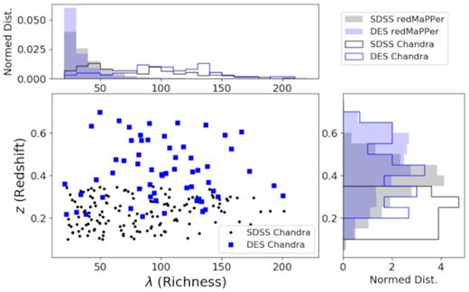
Normalized redshift and richness distributions of the SDSS (black) and DES (blue) redMaPPer clusters matched to archival Chandra observations. The X-ray matched clusters have much higher richnesses than the general redMapper sample, although we do not find significant richness dependence of the results presented in the paper.
![The Rλ [$R_\lambda =(\lambda /100)^{0.2} \, h^{-1}\, {\rm Mpc}$] scaled offset distribution between the redMaPPer centres and the X-ray emission peaks for the redMaPPer SDSS and DES samples from the Chandra archival observations, with the inset zooming on the mis-centred component, starting at roffset/Rλ = 0.05. The distribution can be fitted with two components – a concentrated component that represents the well-centred redMaPPer clusters, and an extended component that represents the mis-centred redMaPPer clusters. The best-fitting SDSS offset model is shown as the solid lines (black: well-centred model, red: mis-centred model), with the shaded regions representing the uncertainties.](https://oup.silverchair-cdn.com/oup/backfile/Content_public/Journal/mnras/487/2/10.1093_mnras_stz1361/1/m_stz1361fig3.jpeg?Expires=1750239259&Signature=nUC8-~DsGrDs2GnsmrVMfNv-EEiOXTbqZ1z9XnnSq8llo6NIO1oj8RzeWB3JXVTNExsjxLR9YttocptH8pl4C-aqMvXzE5TER1OcyQQDg84OZaBa1GfYVZjJvVjFevjDqRb3eAIQfmwXI7SnmtejVOH2k7AXoBOcjHqgtWWmyFLbIqfGW8Pji7J5H8BLPo1~gCK~iKwRAGbRM48NdX6QX4s2V6Ui5QjMjBgUJB4YLnBagxLn8b2tBydPlc1YXtK9RFEBBEstbBQWM7~nhJLxcGxMOUkOPJSj-ABoEjRKOb3PHv4zgm2kaABDQQs8lKVn0iYvMa602-~bkkT3MuDYKA__&Key-Pair-Id=APKAIE5G5CRDK6RD3PGA)
The Rλ [|$R_\lambda =(\lambda /100)^{0.2} \, h^{-1}\, {\rm Mpc}$|] scaled offset distribution between the redMaPPer centres and the X-ray emission peaks for the redMaPPer SDSS and DES samples from the Chandra archival observations, with the inset zooming on the mis-centred component, starting at roffset/Rλ = 0.05. The distribution can be fitted with two components – a concentrated component that represents the well-centred redMaPPer clusters, and an extended component that represents the mis-centred redMaPPer clusters. The best-fitting SDSS offset model is shown as the solid lines (black: well-centred model, red: mis-centred model), with the shaded regions representing the uncertainties.
3 THE X-RAY REDMAPPER OFFSET
3.1 Model
In this paper, we use the X-ray peaks as the cluster fiducial centre, and model the offsets between X-ray peaks and redMaPPer centres to characterize the redMaPPer centring distribution.
Centring offset parameter constraints (equation 1) for the Chandra DES and SDSS redMaPPer samples.
| ρ | σ | τ | |
| Prior | [0.3, 1] | [0.0001, 0.1] | [0.08, 0.5] |
| Chandra SDSS posterior | |$0.678^{+0.035 }_{ -0.051}$| | |$0.0156^{+0.0026}_{ -0.002}$| | |$0.179^{+0.021 }_{ -0.021}$| |
| Chandra DES posterior | |$0.835^{+0.112 }_{ -0.075}$| | |$0.0443^{+0.0231}_{ -0.0094}$| | |$0.166^{+0.111}_{ -0.042}$| |
3.2 Model constraints
The aforementioned X-ray redMaPPer offset model is constrained separately for the Chandra SDSS and DES redMaPPer samples. Table 1 lists and Fig. 4 shows the posterior constraints of the model parameters including the correctly centred fraction ρ, and the mis-centred characteristic offset τ, as well as the characteristic redMaPPer X-ray offset, σ. The SDSS sample yields higher precision because of the larger sample sizes. The fraction of well-centred clusters ρ and the mis-centring offset τ for the mis-centred clusters are mildly different from the DES redMaPPer sample which displays a hint of having a higher fraction of well-centred clusters at a 1.5σ significance level. For the well-centred clusters, the characteristic redMaPPer X-ray offset, σ, of the DES sample is larger than the respective parameter of the SDSS sample, reflecting the limited angular resolution of X-ray peak identification and the higher redshift range of the DES sample (and therefore lower physical separation resolution of the DES X-ray peak identification).
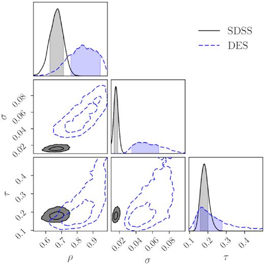
Centring offset parameter constraints (equation 1) for the Chandra DES (blue) and SDSS (grey) redMaPPer samples. About |$70{{\ \rm per\ cent}}$| of the DES and SDSS redMaPPer clusters appear to be well centred in both samples (indicated by the ρ parameter). For the mis-centred clusters, their mis-centring offsets is characterized by a Gamma distribution with a characteristic offset (the τ parameter) around 0.18 Rλ.
The redMaPPer algorithm computes a centring probability, Pcen, as an indicator of whether or not the selected central galaxy is the right choice. We do not find the values of Pcen to accurately reflect the centring statistics of the redMaPPer sample. Specifically, we study the dependence of the centring performance by separately constraining the centring model of the redMaPPer SDSS sample in two Pcen ranges, ≥0.9 and <0.9, respectively. Clusters of Pcen ≥ 0.9 have centring fraction of 0.76 ± 0.05 while clusters of Pcen < 0.9 have a notably lower centring fraction of 0.49 ± 0.09. Although a larger Pcen value does indicate a better centring performance, it does not reflect the real centring fractions at the face values.
We have tested the dependence of the centring parameters through constraining the model with the SDSS sample in different ranges of richnesses, X-ray temperatures or luminosities, and for serendipitous versus targeted observations. We do not find significant differences in the centring parameter constraints. A larger set of X-ray observations would be needed to reveal any trends.
Interpretation of the results from this centring offset characterization depends on the adopted models. Different functional forms of the mis-centring offset – a Rayleigh distribution for the mis-centred component, and a Gaussian distribution for the well-centred clusters – have been attempted in previous studies (Saro et al. 2015; Rykoff et al. 2016; Hikage et al. 2017). We have tested alternative models (listed in Table 2) for the mis-centring and centring distributions with the Chandra SDSS sample. As the common parameter shared across different models, the well-centred cluster fraction, ρ, is consistently constrained to be in the range of 64 per cent to 70 per cent for SDSS.
Alternative offset models and constraints derived with the Chandra SDSS redMaPPer sample, and DIC comparisons to the nominal model in this paper.
| Name | Model | Constraints | DIC − DICnominal |
|---|---|---|---|
| Gaussian | P(x|ρ, σ, τ) = ρPcent + (1 − ρ)Pmiscent | |$\rho =0.64^{+0.05 }_{ -0.05}$| | 19.0 |
| |$P_\mathrm{cent}(x | \sigma) = \frac{2}{\sqrt{2\pi }\sigma } \mathrm{exp}(- \frac{x^2}{2\sigma ^2})$| | |$\sigma =0.0177^{+0.0025 }_{ -0.0020}$| | ||
| |$P_\mathrm{miscent}(x | \tau) = \frac{x}{\tau ^2} \mathrm{exp}(- \frac{x}{\tau }).$| | |$\tau =0.161^{+0.021 }_{ -0.016}$| | ||
| Rayleigh | P(x|ρ, σ, τ) = ρPcent + (1 − ρ)Pmiscent | |$\rho =0.70^{+0.05 }_{ -0.04}$| | 4.4 |
| |$P_\mathrm{cent}(x | \sigma) = \frac{1}{\sigma } \mathrm{exp}(- \frac{x}{\sigma })$| | |$\sigma =0.0185^{+0.0025 }_{ -0.0023}$| | ||
| |$P_\mathrm{miscent}(x | \tau) = \frac{x}{\tau ^2} \mathrm{exp}(- \frac{x^2}{2\tau ^2}).$| | |$\tau =0.323^{+0.029 }_{ -0.024}$| | ||
| Full gamma | P(x|ρ, σ, τ, k) = ρPcent + (1 − ρ)Pmiscent | |$\rho =0.64^{+0.07 }_{ -0.05}$| | 1.85 |
| (four parameters) | |$P_\mathrm{cent}(x | \sigma) = \frac{1}{\sigma } \mathrm{exp}(- \frac{x}{\sigma })$| | |$\sigma =0.015^{+0.0027 }_{ -0.003}$| | |
| |$P_\mathrm{miscent}(x | \tau , k) = \frac{x^{k-1}}{\Gamma (k) \tau ^k} \mathrm{exp}(- \frac{x}{\tau })$| | |$\tau =0.21^{+0.07 }_{ -0.05}$| | ||
| |$k=1.0^{+0.83 }_{ -0.0}$| | |||
| Cauchy | P(x|ρ, σ, τ) = ρPcent + (1 − ρ)Pmiscent | |$\rho =0.645^{+0.05 }_{ -0.05}$| | 14.2 |
| |$P_\mathrm{cent}(x | \sigma) = \frac{1}{\sigma } \mathrm{exp}(- \frac{x}{\sigma })$| | |$\sigma =0.014^{+0.0028 }_{ -0.0022}$| | ||
| |$P_\mathrm{miscent}(x | \tau) = \frac{x\tau }{(x^2+\tau ^2)^{1.5}}$| | |$\tau =0.14^{+0.04 }_{ -0.03}$| |
Notably, when adopting a Rayleigh distribution for the mis-centred component, our SDSS posterior values on the well-centred cluster fraction, ρ, and the mis-centred characteristic offset, τ are highly consistent with the previous study in Hikage et al. (2017) which adopts a similar model and is based on a similar SDSS redMaPPer catalogue. The posterior precision of the parameters has improved significantly in our analysis.
3.3 Model validation
We check the model goodness-of-fit with a posterior prediction test. Specifically, we compare the fractions of clusters in an offset range from the data to the predictions from the constrained models. The procedures are as the follows.
From the measurements of x = roffset/Rλ, record the number of clusters with offsets larger than a comparison value x0.
Take one set of model parameters, ρ, σ, and τ from the MCMC posterior constraints, denoted as ρi, σi, and τi. Randomly draw a set of centring offsets, {xij}, from the offset model (equation 1) with the above set of posterior model parameters. The number of random draws should match the size of the X-ray-redMaPPer sample being tested.
With the above set of centring offsets sampling, {xij}, record the number of offsets larger than a comparison value x0, N(xij > x0).
Repeat the process for each set of ρ, σ, and τ values from the MCMC posterior chain and acquire the distribution of N. This is the posterior prediction on the number of clusters with offsets larger than the comparison value x0.
Compare the number from data to this posterior prediction. We expect a two-sided P-value, defined as the minimum of the fractions of the posterior predictions above and below the data, to be larger than 0.025.
We use the above process to evaluate the goodness of the model at offsets larger than 0.1, 0.5, and 1 Rλ. Fig. 5 shows the posterior predictive distribution of these offset ranges. For both the SDSS and DES redMaPPer samples, the prediction from the model and its respective model constraints well match the measurements from the data in these small, medium, and large offset ranges, with the two-sided P-values being 0.35, 0.37, and 0.18 for SDSS and 0.11, 0.25, and 0.17 for DES.
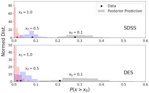
Posterior predictive check of the centring offset model. We show the predictions on the fraction of clusters in different offset ranges (x > 0.1, x > 0.5, and x > 1.0) from the offset model sampling the posterior constraints (histograms). These predictions agree with the measurements from data (solid squares) for both the SDSS and DES models and data.
4 MIS-CENTRING IMPACT ON RICHNESS SCALING RELATION
When a cluster is mis-centred, the redMaPPer richness estimation may become biased, and the bias depends on the mis-centring offset. In this section, we use the redMaPPer catalogue itself to constrain a model that describes the bias of λ upon a mis-centring offset.
As mentioned in Section 3, the redMaPPer algorithm selects the five most probable central galaxies and stores the λ estimations computed at each of the centres. The default redMaPPer centre is chosen as the one with the highest centring probability. We make use of this information to construct a richness shift versus offset model.
Assuming that there existed a redMaPPer catalogue with the most probable centres always being the correct ones, the λ estimations computed at the other four centres will be affected by the mis-centring effect. The λ bias between the real centre and each of the four remaining centre candidates, and the positional offsets between them, can be used to constrain a λ versus centring offset model.
We use the lambda offsets between the second and the first (redMaPPer default centre) most likely centres, and the distance offset between them, to model the richness versus centring offset (Section 4.1). The model is further validated with X-ray data (Section 4.2).
4.1 Model and model constraints
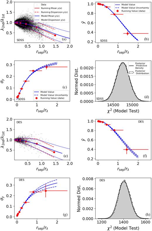
The richness versus offset distributions and models. The cluster richness tends to be biased lower by mis-centring (a, e), and the mean of the bias can be characterized by a Gaussian function (b, f). The biases have large dispersions (c, g), which can be further characterized by an arctan function (c, g). Posterior predictive checks show that the models are tightly constrained from the data and fit the data well (d, h).
The process of evaluating the above model goes as follows:
We compute the separation between the first and the second most probable centres, rsep, assuming the cluster photometric redshift from the redMaPPer algorithm for both of the galaxies. We scale rsep as rsep/rλ to become quantity x.
We compute the relative λ offset between the first and the second most probable centres as y = λ2nd/λ1st.
We repeat the above process for each cluster i in the redMaPPer catalogue, acquiring a measurement data set {xi} and {yi}. This data set is shown in Fig. 6.
With the above measurement data set, we constrain the model parameters of y with the following likelihood: |$\mathcal {L}=\sum _{i, x_i\lt 0.1}\big (-\frac{[y_i-\bar{y}(x_i)]^2}{2\sigma ^2_y(x_i)}-\mathrm{ln}[\sigma _y(x_i)] \big)$|. The likelihood is sampled with an MCMC algorithm.
Note that only the data points with xi > 0.1 are used in the fitting process. This helps eliminate overfitting at small x, and improves the fitting results at large x.
The same measurements and modelling processes are performed for the SDSS and DES redMaPPer catalogues separately. Fig. 6 shows the data points as well as the best-fitting models in the first two columns. For comparison, the red lines/points are the data running averages and running dispersions in the x bins (bin widths indicated by the x error bars in the second column). The MCMC posterior constraints are shown in Fig. 7 and listed in Table 3. α does not appear to be covariant with a or b, but a and b appear to be highly covariant.
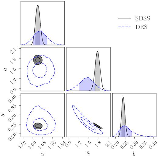
Parameter constraints for the lambda offset versus centring offset model. See Section 4.2 for details.
Parameter constraints for the lambda offset versus centring offset model as in |$\bar{y}(x)=\mathrm{exp}(-x^2/\sigma ^2)$| and σy(x) = a × arctan(bx).
| SDSS α | SDSS b | SDSS a | |
|---|---|---|---|
| Prior | (0, 10) | (0, 10) | (0, 10) |
| Posterior | 1.64 ± 0.02 | 1.76 ± 0.07 | 0.241 ± 0.008 |
| DES α | DES b | DES a | |
| Prior | (0, 10) | (0, 10) | (0, 10) |
| Posterior | 1.66 ± 0.06 | 1.43 ± 0.22 | 0.26 ± 0.04 |
| SDSS α | SDSS b | SDSS a | |
|---|---|---|---|
| Prior | (0, 10) | (0, 10) | (0, 10) |
| Posterior | 1.64 ± 0.02 | 1.76 ± 0.07 | 0.241 ± 0.008 |
| DES α | DES b | DES a | |
| Prior | (0, 10) | (0, 10) | (0, 10) |
| Posterior | 1.66 ± 0.06 | 1.43 ± 0.22 | 0.26 ± 0.04 |
Overall, the impact of mis-centring on cluster richness is mild with a low scatter at small mis-centring offset, but grows with a larger offset, reaching a bias ratio λmiscentred/λtrue of 0.5 at rsep/Rλ ∼ 1.40.
4.2 Model validation with X-ray centres
As a test of the richness offset model, we make use of the Chandra-redMaPPer samples (Section 2.3) and compare the X-ray peak redMaPPer centred λ to the prediction from the model. We rerun the redMaPPer λ algorithm with the X-ray peaks as the cluster centres. The procedures are equivalent to the original λ estimation with the exception of a ‘percolation’ process (Rykoff et al. 2014), which re-evaluates λ upon masking neighbouring redMaPPer clusters. The λ estimations on X-ray peaks do not go through the ‘percolation’ process as the run does not consider redMaPPer clusters not present in the X-ray sample. In this test, to ensure that the ‘percolation’ process is negligible, we remove clusters whose λ changed by 10 per cent in the initial redMaPPer percolation process.3
We calculate the λ offsets versus the distance offsets between the X-ray peaks and redMaPPer centres. The λ offsets are calculated as yx = λRM/λxray, and the corresponding X-ray and redMaPPer mis-centring offsets as xx = rsep/rλ, where rλ is evaluated with the X-ray centred λ. Clusters of centring offsets xx less than 0.1 are considered well-centred (a similar cut is applied when deriving the model in Section 4.1) and do not enter the test. In Fig. 8, we show the derived λ and centring offsets from the X-ray observations. The constrained models in Section 4.1 appear to be qualitatively consistent with these offsets.
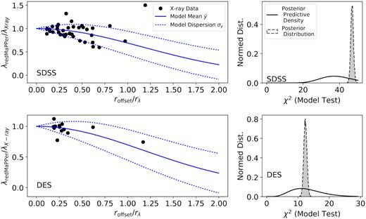
The shift in richness when the richness is estimated at the X-ray centres rather than the redMaPPer centres (first column). The lambda versus centring offset models derived from the redMaPPer catalogue are shown as blue solid and dashed lines. Posterior predictive checks (second column) show that the richness shifts estimated at the X-ray centres adhere to the models derived from the redMaPPer catalogue (see Section 4.2 for details).
We perform Bayesian posterior predictive assessment on the fitness of the model following the process in Gelman, Meng & Stern (1996) and Meng (1994). The process includes calculating a posterior predictive p-value (PPP value) which is the classical p-value averaged over the posterior model parameter distribution. With the posterior distribution of α, a and b sampled with the MCMC method, the procedure goes as follows:
Take one set of α, a, and b from the MCMC posterior constraints, donated as αj, aj, and bj.
Calculate the χ2 discrepancy for αj, aj, and bj, denoted as |$\chi ^2_j$|.
Repeat the process for each set of α, a, and b values from the MCMC posterior chain.
For each |$\chi ^2_j$|, randomly draw a value, qj, from a standard χ2(n) distribution. For the posterior set of |$\lbrace \chi ^2_j, q_j\rbrace$|, record the fraction of |$\chi ^2_j \ge q_j$| as Pb1, and the frequency of |$\chi ^2_j \le q_j$| as Pb2. We use a two sided p-value definition, that Pb = min(Pb1, Pb2) as the PPP value.
We compute the posterior χ2 discrepancy given X-ray {yx, xx} observations shown in Fig. 8. The posterior χ2 discrepancy values are expected to occupy a highly probable interval of a chi-squared distribution χ2(n) (posterior predictive density), with the degree of freedom n matching the number of {yx, xx} observations from X-ray peak centres. This appears to be the case for both the SDSS and DES X-ray redMaPPer sample. The Bayesian posterior predictive P-values (PPP values) are 0.18 and 0.50 respectively for the SDSS and DES X-ray redMaPPer samples. Both of the PPP values are above a 0.025 model rejection threshold, indicating consistency between the constrained models and the offsets derived with X-ray peak centres.
We also compute the posterior χ2 discrepancy for the original {yi}, {xi} observations that are used to constrain the model. The distributions of |$\lbrace \chi ^2_j\rbrace$| are shown as the grey shaded histogram in Fig. 6, along with the probability density of a chi-squared distribution, χ2(n), for comparison. The distribution of |$\lbrace \chi ^2_j\rbrace$| is in good accordance with the expected χ2(n) distribution, for both the SDSS and DES redMaPPer samples, indicating the goodness of the fit and tightness of the model parameter constraints. The PPP values for the SDSS and DES samples are 0.50 and 0.49, respectively, matching the expectation of a well-posited model.
Note that when deriving the model, the available redMaPPer catalogues already have imperfect centre selections. According to the previous section, the majority (∼70 per cent) of the clusters in the redMaPPer catalogue are correctly selected. We have attempted to select clusters with a higher centring probability (using the redMaPPer Pcen quantity), but the samples selected on Pcen display a hint of performing slightly worse in the validation test with X-ray data. Because of a concern that this Pcen selection may have biased the cluster sample, and that the selection still cannot ensure a 100 per cent well centred subsample, we do not apply the selection in this paper and emphasize on our derived model passing the validation test with X-ray data. In the future, it would be desirable to quantify the richness offset model with X-ray centred richness when larger X-ray redMaPPer clusters become available.
5 IMPLICATIONS FOR DES CLUSTER COSMOLOGY
5.1 Mis-centring model in DES cluster weak lensing analysis
5.2 Sensitivity of cluster mass estimation to the mis-centring model
We determine the sensitivity of the mass calibration to variations in the values of the mis-centring parameters. To do so, we create a fiducial mass profile and analyse how much the measured masses deviate from the truth if the mis-centring model is inaccurate. Following the recipe in McClintock et al. (2019), the fiducial mass profile model combines an NFW profile and a two-halo model of M200m = 1014 M⊙, concentration of 5 and Rλ = 1 Mpc. We compute the mis-centred lensing signal by adopting fiducial values ρ = 0.68 and τ = 0.15. We fit this synthetic weak lensing data with a minimum χ2 method assuming a range of values for both ρ and τ, and measure the bias of the best-fitting mass and concentration as a function of these two parameters. The fitting process is restricted to the 0.2–30 Mpc radius range as in the DES Y1 weak lensing study (McClintock et al. 2019) and the profile measurement uncertainty is assumed to be due to shape nose only, and therefore scales with radius as r−1.
Fig. 9 shows the best-fitting mass and concentration parameters as a function of ρ and τ. We find that the best-fitting mass is insensitive to the assumed ρ value, whereas the recovered concentration is biased. Allowing the concentration parameter to vary effectively decouples the recovered mass from ρ. By contrast, variations in τ have a non-negligible impact on the best-fitting mass. Uncertainties in τ at a level of ±0.04, comparable to the constraint in this paper, results in a mass uncertainty of ±0.015 dex.4
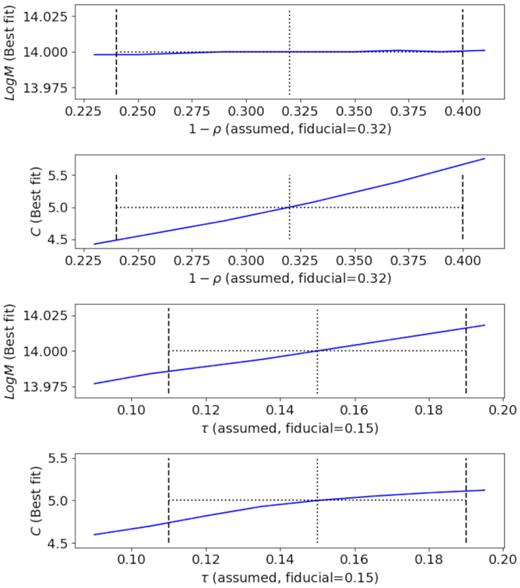
We explore how inaccurate knowledge of the mis-centring model parameters affects the accuracy of cluster mass and concentration estimations in cluster lensing studies. A fiducial mass profile is created using the prescription in McClintock et al. (2019) with a fiducial set of mis-centring parameters. Through comparing to the fiducial mass profile, the best-fitting mass and concentrations are estimated for different assumed values of the mis-centring model parameters, ρ and τ. We find that the mass estimation is robust under inaccurate assumptions of ρ, but susceptible to inaccuracy in τ. The concentration parameter, on the contrary, is more susceptible to the inaccuracy of ρ than τ. The vertical lines indicate parameter ranges comparable to those in McClintock et al. (2019).
These results are in qualitative agreement with the results of McClintock et al. (2019), though computed with two important methodological differences. Specifically: (1) McClintock et al. (2019) has considered more systematic effects other than mis-centring, including using a semi-analytic covariance matrix (Gruen et al. 2015), and accounting for boost-factor corrections (Varga et al. 2018). These changes will affect the relative weighting of radial inner to outer scales, thereby impacting the sensitivity of the mass posteriors to the mis-centring parameters. (2) When constraining the richness-mass scaling relation parameters, McClintock et al. (2019) treats the mis-centring parameters for each richness and redshift bin as independent, which reduces the relative importance of mis-centring in their analysis. Together, these differences reduce the sensitivity of the scaling relation amplitude from the 0.015 dex we estimated here to 0.78 per cent, as quoted in McClintock et al. (2019). Nevertheless, it is clear from fig. 10 in McClintock et al. (2019) that the mass posterior in a single bin is largely insensitive to ρ, but is degenerate with τ, as illustrated in our toy model analysis above.
These conclusions, however, rely on the assumption that the cluster mass profile is not correlated with the cluster mis-centring effect in optical data. Future cluster lensing analysis may wish to further investigate this assumption, e.g. through examining the cluster mass distribution in X-ray selected clusters (Das et al., private communication).
5.3 Cluster abundance
The λ offset caused by cluster mis-centring introduces bias and scatter into the lambda–mass scaling relation. We study the scatter increase with a test based on a N-body dark matter simulation (Habib et al. 2016). Richnesses are prescribed to each of the simulation dark matter haloes following the richness–mass relation in Saro et al. (2015), with a richness scatter, σlnλ|M, of 25 per cent. We perturb the assigned richnesses with the Chandra SDSS offset model presented in Section 3 and the richness bias model presented in this section, and find the richness scatter, σlnλ|M to increase by 2 per cent.
The bias and scatter manifest themselves in the number count of clusters selected by λ, which is a fundamental input to cluster abundance cosmology. Mis-centring tends to lower the richness estimation and the numbers of clusters above a richness threshold selected by the mis-centred richnesses would be lower than those selected by richnesses without mis-centring. The average mass of the clusters selected by the mis-centred richnesses tend to be higher. Testing with simulations shows that the numbers of clusters selected by the mis-centred richnesses is lower by |${\sim } 2{{\ \rm per\ cent}}$|, and the average cluster masses increase by |${\sim }0.5{{\ \rm per\ cent}}$|. Costanzi et al. (2018) estimates these shift to have negligible effects for SDSS and DES Y1 cluster cosmology constraints since they are significantly smaller than the remaining systematic uncertainties of cluster abundance and mass estimations. Nevertheless, Costanzi et al. (2018) and the DES Collaboration (in preparation) corrected the data vectors with the factors listed above to account for the mis-centring effect. Future cluster cosmology analysis in the coming years of DES and LSST may wish to explicitly incorporate the mis-centring richness relations as the mis-centring effect on cluster abundance becomes more substantial compared to the statistical uncertainty.
6 CENTRING STUDY WITH XMM DATA
During the preparation of this paper, an additional sample of redMaPPer clusters (SDSS and DES) with archival X-ray observations from the XMM–Newton space telescope became available. As the centring analyses in this paper are optimized for Chandra observations, especially the centring offset model for well-centred clusters is optimized for Chandra PSFs, we do not attempt to combine the XMM and Chandra observations in the modelling processes. Rather, we use the XMM defined X-ray centres to explore the robustness of the fits presented in Section 3. The sample selection and the XMM data analysis methods are described in Section 6.1, and Section 6.2 describes the centring comparison results from XMM.
6.1 X-ray data processing
The redMaPPer–XMM joint samples (SDSS and DES) were constructed as follows. First, the redMaPPer centroids were compared to the aim points of observations in the XMM public archive.5 redMaPPer clusters with centroids falling outside 13 arcmin of an aim point were excluded from the samples. Secondly, the mean and median XMM exposure time was determined within a 10 arcsec radius of the redMaPPer centroid. For this we used exposure maps produced by the XMM Cluster Survey (XCS, Lloyd-Davies et al. 2011). Any redMaPPer clusters with mean exposure times of <3 ks, and/or median exposure times of <1.5 ks, were excluded from the samples. We note that the median filter was necessary because some clusters straddle both active and inactive regions of the field of view (FOV), e.g. those lying close to the FOV edge. If a given cluster was observed multiple times by XMM, only the observation with the longest exposure time, at the redMaPPer centroid, was used in subsequent analyses. Third, the remaining redMaPPer cluster centroids were compared to the list of extended sources detected using the XCS Automated Pipeline Algorithm (XAPA). Any redMaPPer clusters lying further than 2 h−1 Mpc (assuming the redMaPPer redshift) of such a source were excluded from the samples. At this stage, the SDSS and DES redMaPPer–XCS samples comprised of 356 and 282 clusters, respectively.
The X-ray peaks for the clusters in the redMaPPer–XMM joint samples were then determined using a method that closely follows that used for the Chandra analyses, as described in Section 2.3. An initial peak location was found in the respective merged (PN, MOS1, MOS2) XMM image, after smoothing with a σ = 50h−1 kpc Gaussian (assuming the redMaPPer redshift). As with the Chandra analysis, other sources (i.e. those assumed not to be associated with the redMaPPer cluster) are masked out before the smoothing takes place. For this, we use the XAPA source catalogue of point-like sources. If there are multiple XAPA extended source within the image, then only the one closest to the redMaPPer centroid is left unmasked. The peak location is then the brightest pixel in the masked, smoothed image, within a radius 1.5 × Rλ of the RM position.
The initial peak selection was occasionally erroneous. For example when there was a very bright point source in the XMM FOV. Such sources ‘bleed’ into the surrounding region of the detector, meaning that the default point source mask size was not large enough remove them completely. Such cases were easily identified by eye using SDSS (or DES) and XMM ‘postage stamp’ images. Most of these cases could be corrected by adjusting the size of the point source mask, and then re-running the peak finding script. However, for some, the point source ‘bleeding’ was so pronounced that the respective cluster had to be removed from the redMaPPer–XMM joint sample. Another reason for the initial peak being erroneous was the mis-percolation issue described in Section 2.3. The mis-percolation cases were also identified using eye-ball checks. For these it was necessary to adjust the extended source mask, so that the closest source was now masked, but the second closest was not.
Once the second run of peak finding has been completed (and the new peak positions have been confirmed by eye), the remaining clusters were eye-balled again. At this stage, more redMaPPer clusters were removed from the sample: (i) those where the XAPA extended source is clearly not associated with the redMaPPer cluster (i.e. it is a foreground background cluster in projection), and (ii) those where the redMaPPer central galaxy falls in an XMM chip gap. After the various cuts described above, the SDSS–XCS and DES–XCS samples contained 248 and 109 sources, respectively.
We further apply off axis angle and SNR cuts to the XMM samples. The SNR was determined in the same way as for the Chandra sample i.e. within 500h−1 kpc, using 0.5–2.0 keV XMM images. For the XMM-SDSS sample, we require the detections S/N to be >6.5, and the redMaPPer centres to be within 8.5 arcmin of the aim point (or 6.5 arcmin away from the FOV edge assuming a 15 arcmin FOV radius). For the XMM-DES sample, we again require the detections S/N to be >6.5, but allow the redMaPPer centres to be up to 10.5 arcmin of the aim point. The FOV cuts ensure that the corresponding redMaPPer centres are more than 500 kpc away from the FOV edge at z = 0.1 for the SDSS sample, or at z = 0.2 for the DES sample. The S/N cuts were imposed to match the 6.5 S/N cuts in the Chandra analysis. With these FOV and S/N cuts, the final SDSS and DES XMM samples contain 163 and 66 clusters, respectively. Fig. 10 shows their richness and mass distributions.
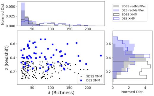
Redshift and richness distributions of the SDSS (black) and DES (blue) redMaPPer clusters matched to archival XMM observations.
Further details of the redMaPPer–XMM joint sample development, the peak measurements, the signal-to-noise estimation and the individual mis-percolation cases can be found in Giles et al. (in preparation).
6.2 The XMM–Chandra and XMM–redMaPPer offsets
A subsample of the redMaPPer clusters, 54 in the SDSS sample, and 25 in the DES sample, are analysed by both the XMM and Chandra analyses. With these overlapping cases, we compare the XMM peak measurements to those from Chandra. Fig. 11 shows the offset distribution between XMM and Chandra peak identifications for the same redMaPPer clusters, scaled by their Rλ. The XMM and Chandra peak identifications are highly consistent: their separations are within 0.05 Rλ for 53/54 of the overlapping SDSS clusters, and 20/25 of the overlapping DES clusters. The separations have a wider distribution for the DES redMaPPer sample reflecting its higher redshift range, and hence higher X-ray peak identification uncertainties in terms of physical distances.
![The Rλ [$R_\lambda =(\lambda /100)^{0.2} \, h^{-1}\, {\rm Mpc}$] scaled offset distribution between the Chandra and XMM peak identifications for the same redMaPPer clusters.](https://oup.silverchair-cdn.com/oup/backfile/Content_public/Journal/mnras/487/2/10.1093_mnras_stz1361/1/m_stz1361fig11.jpeg?Expires=1750239259&Signature=jVICpoGdt0PLvKTpsZ~69H4MOdhZhn9HvBcxDPd5zXNh3zhNAJo25ActK4oLKRiMpEGuJJKi5iGzxdSA2aPMof6dV81QWgNKKRr8fNxZY5bCmZ~6w~IHnfUA9WWNlqLd7WXRpoupiHZ5TxbNTqB3T67F-DvQ72LMk15xSxxT~yX2Tao04HCg7dAR8rreIk7wYeF2e8fdsKAj4~1TFJhhefct5JOhNNQy581ANM-zRlkiRUgqMrfoptx0ul6Y~mHxYQwocVPlGvCK9rrnJsyouqJr3J1cUNANoHyhh4G1nSvfZ10s5NgVgdDmnhibCSxHuqF9ReU2YLdM507XNJmipw__&Key-Pair-Id=APKAIE5G5CRDK6RD3PGA)
The Rλ [|$R_\lambda =(\lambda /100)^{0.2} \, h^{-1}\, {\rm Mpc}$|] scaled offset distribution between the Chandra and XMM peak identifications for the same redMaPPer clusters.
Given the consistency between XMM and Chandra X-ray peak identifications, we constrain the redMaPPer centring offset model proposed in Section 3 with the XMM peaks. Figs 12 and 13 respectively show the offset distributions between the XMM peaks and the redMaPPer centres for the SDSS and DES samples, with comparisons to their corresponding Chandra offset distributions. Figs 14, 15, and Table 4 show the model parameter constraints from these XMM samples. The σ parameter in our redMaPPer centring offset model (equation 1) represents the X-ray peak offset to cluster central galaxy for well-centred clusters, which is further smeared by X-ray peak identification uncertainty and X-ray telescope PSFs. Since σ is in the unit of physical distance, the σ difference can be driven by the different angular resolutions of XMM and Chandra at low redshift, and other X-ray peak identification uncertainties, and X-ray peak-galaxy centre separations at higher redshift. Hence, we do not expect this parameter to agree between XMM and Chandra, and the σ difference is especially larger for the lower redshift SDSS redMaPPer samples. For the other two parameters of the model, ρ and τ, which respectively represent the well-centred fractions of redMaPPer and the centring offset of mis-centred redMaPPer clusters, the constraints from XMM are consistent with those from Chandra for both the SDSS and DES redMaPPer samples within two standard deviations.
![The Rλ [$R_\lambda =(\lambda /100)^{0.2} \, h^{-1}\, {\rm Mpc}$] scaled offset distribution between the redMaPPer centres and the X-ray emission peaks for the redMaPPer SDSS samples from the XMM archival observations. The distribution can be fitted with two components – a concentrated component that represents the well centred redMaPPer clusters, and an extended component that represents the mis-centred redMaPPer clusters. The best-fitting SDSS offset model is shown as the solid lines (black: well-centred model, red: mis-centred model), with the shaded regions representing the uncertainties. As a comparison, we also show the corresponding offset distribution from the analysis with Chandra archival data (blue dashed histogram).](https://oup.silverchair-cdn.com/oup/backfile/Content_public/Journal/mnras/487/2/10.1093_mnras_stz1361/1/m_stz1361fig12.jpeg?Expires=1750239259&Signature=WIRLNzX4LIdPabIrKyi~U087a6AcJq0-wFkzOYg9vBEss1u40Ixz1NDbcX2FX0WaejTq687VPoHvSmlOJmA1PCrqQlOVvZ3~yHhLL8k6sCh2v47tyqhUdPFo6-68zgqtsmjOsndDkvPLTaBRD04SDTV1~iOgd67YQ-lmyrHq7BvEz8KCVi8hO89mCvJDrAXT0CmEjNhHG5EA8HQ3wCCEbsSme4mwgBTjPmyYTe48cFpiq95pCHoefytE40PgpJORNJwg~7-vw1H7BLJNA9lLfL2N6sIKSML~XHynOnLUNgPwLSRH5mLjcwj-YpB1QQkpGxJVvBEJZFhz9gBCeTAmhQ__&Key-Pair-Id=APKAIE5G5CRDK6RD3PGA)
The Rλ [|$R_\lambda =(\lambda /100)^{0.2} \, h^{-1}\, {\rm Mpc}$|] scaled offset distribution between the redMaPPer centres and the X-ray emission peaks for the redMaPPer SDSS samples from the XMM archival observations. The distribution can be fitted with two components – a concentrated component that represents the well centred redMaPPer clusters, and an extended component that represents the mis-centred redMaPPer clusters. The best-fitting SDSS offset model is shown as the solid lines (black: well-centred model, red: mis-centred model), with the shaded regions representing the uncertainties. As a comparison, we also show the corresponding offset distribution from the analysis with Chandra archival data (blue dashed histogram).
![The Rλ [$R_\lambda =(\lambda /100)^{0.2} \, h^{-1}\, {\rm Mpc}$] scaled offset distribution between the redMaPPer centres and the X-ray emission peaks for the redMaPPer DES samples from the XMM archival observations. The distribution can be fitted with two components – a concentrated component that represents the well centred redMaPPer clusters, and an extended component that represents the mis-centred redMaPPer clusters. The best-fitting DES offset model is shown as the solid lines (black: well-centred model, red: mis-centred model), with the shaded regions representing the uncertainties. As a comparison, we also show the corresponding offset distribution from the analysis with Chandra archival data (blue dashed histogram).](https://oup.silverchair-cdn.com/oup/backfile/Content_public/Journal/mnras/487/2/10.1093_mnras_stz1361/1/m_stz1361fig13.jpeg?Expires=1750239259&Signature=GZ7jhaxx9~eGc7Ac4IWk0bdgBWyShOBp5-hsDvwJFPbrd5PYOvbDvbET3q22K7tyUsD62NmSssJYltPdCSYZdS7FXHcsxX5JAPAaAlLikLL-Z6aw8odWL9qqtjQhB9Iy7-XON-6ywZTi-m0WhlBDEFJED38tVKkBmF8h0LnV9pGh1-dN4DF8m7k365xtP5q0vSp8P84GZcxDinocOsXK9zRaYUUqyu2-FpSymfq~4IPFGt03WCoLjTeO2Uww7AMAVU02iUQU7EfwW7-f4-YMkKY9iBTgEWHWjjvaFlWf-8uPpTM3~z9wJ4GwkclPahIZZO-Wq-R2DECbopIW6gfi6w__&Key-Pair-Id=APKAIE5G5CRDK6RD3PGA)
The Rλ [|$R_\lambda =(\lambda /100)^{0.2} \, h^{-1}\, {\rm Mpc}$|] scaled offset distribution between the redMaPPer centres and the X-ray emission peaks for the redMaPPer DES samples from the XMM archival observations. The distribution can be fitted with two components – a concentrated component that represents the well centred redMaPPer clusters, and an extended component that represents the mis-centred redMaPPer clusters. The best-fitting DES offset model is shown as the solid lines (black: well-centred model, red: mis-centred model), with the shaded regions representing the uncertainties. As a comparison, we also show the corresponding offset distribution from the analysis with Chandra archival data (blue dashed histogram).
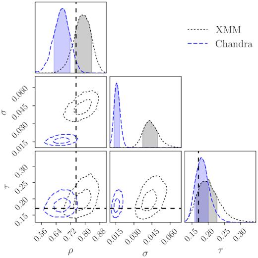
Centring offset parameter constraints (equation 1) for the XMM SDSS (grey) redMaPPer samples. |$76\pm 6{{\ \rm per\ cent}}$| of the SDSS redMaPPer clusters appear to be well centred (indicated by the ρ parameter). For the mis-centred clusters, their mis-centring offsets is characterized by a Gamma distribution with a characteristic offset (the τ parameter) of 0.16 ± 0.03 Rλ. As a comparison, we also show the corresponding model constraints from the SDSS analysis with Chandra archival data (blue). The prior central values adopted in DES cosmological analyses as described in Section 5 are shown as the black dashed lines.
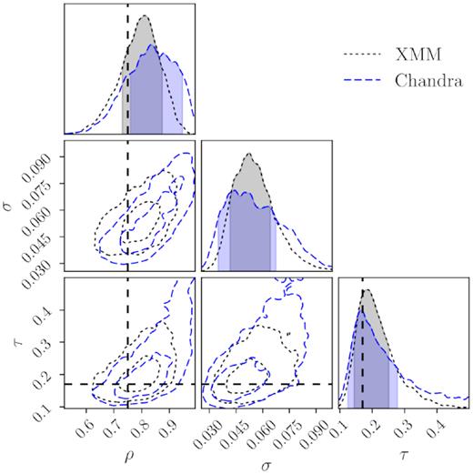
Centring offset parameter constraints (equation 1) for the XMM DES (grey) redMaPPer samples. |$74\pm 10{{\ \rm per\ cent}}$| of the DES redMaPPer clusters appear to be well centred (indicated by the ρ parameter). For the mis-centred clusters, their mis-centring offsets is characterized by a Gamma distribution with a characteristic offset (the τ parameter) of 0.20 ± 0.07 Rλ. As a comparison, we also show the corresponding model constraints from the DES analysis with Chandra archival data (blue). The prior central values adopted in DES cosmological analyses as described in Section 5 are shown as the black dashed lines.
Centring offset Parameter constraints (equation 1) for the XMM DES and SDSS redMaPPer samples.
| ρ | σ | τ | |
| Prior | [0.3, 1] | [0.0001, 0.1] | [0.08, 0.5] |
| XMM SDSS posterior | |$0.781^{+0.055 }_{ -0.038}$| | |$0.0432^{+0.0063}_{ -0.0059}$| | |$0.201^{+0.026 }_{ -0.039}$| |
| XMM DES posterior | |$0.815^{+0.059 }_{ -0.085}$| | |$0.053^{+0.012}_{ -0.011}$| | |$0.185^{+0.066}_{ -0.041}$| |
Notably, no selection cuts in the XMM analysis were made to make its centring model constraints better match the Chandra results, yet their centring offset results are consistent with each other. We conclude that the redMaPPer mis-centring offset modelling presented in this paper are robust upon investigation with archival XMM data.
7 SUMMARY
This analysis makes use of the archival X-ray observations to constrain the centring performance of the redMaPPer cluster finding algorithm. We calibrate the well-centred fraction of redMaPPer clusters for both the SDSS and DES samples with the X-ray emission peaks. The offsets between the redMaPPer centres and X-ray peaks are well modelled by a two-component distribution, which indicates that |$69^{+3.5}_{-5.1}{{\ \rm per\ cent}}$| and |$83.5^{+11.2}_{-7.5}{{\ \rm per\ cent}}$| of the clusters are well centred in the SDSS and DES samples. The offset distribution of the mis-centred redMaPPer clusters are modelled with a Gamma distribution, and cluster mass modelling appears to be more sensitive to the accuracy of these mis-centring offsets than the mis-centring fraction.
With the upcoming DES Year 3 and Year 5 data, we expect the redMaPPer centring constraints to continue improving with ∼ 2 times larger overlapping samples between DES and archival X-ray observations, which may permit us to quantify the dependence of the centring parameters on cluster properties, such as cluster richness, redshift, X-ray temperature, and luminosity. The current improvement has already lowered the cluster weak lensing mass modelling uncertainties due to mis-centring, to the extent of being in-substantial comparing to the other modelling systematic effects. Since mis-centring is often assumed to be uncorrelated with cluster mass distributions in weak lensing analyses, with the anticipated level of improvement, one may wish to investigate the correlations of mis-centring with other cluster lensing systematic effects, such as cluster mass modelling uncertainties, cluster orientation, triaxiality, and projection (McClintock et al. 2019).
The cluster richness estimates tend to be biased lower by mis-centering. In this paper, we propose a richness bias model to describe the effect, which is validated by X-ray centred richness measurements. The richness bias is offset dependent, low for clusters with small mis-centering offset, but larger than 50 per cent for severely mis-centred clusters. Cluster cosmology studies based on full depth DES data or LSST data should explicitly account for this effect to avoid biased cosmological parameter inferences.
Code used in this analysis is available from https://github.com/yyzhang/center_modeling_y1.
ACKNOWLEDGEMENTS
TJ is pleased to acknowledge funding support from DE-SC0010107 and DE-SC0013541. AKR, PG, and SB acknowledge support from the UK Science and Technology Facilities Council via grants ST/P000252/1 and ST/N504452/1, respectively. DG was supported in part by the U.S. Department of Energy under contract number DE-AC02-76SF00515 and by Chandra Award Number GO8-19101A, issued by the Chandra X-ray Observatory Center. We use Monte Carlo Markov Chain sampling in this analyses, which are performed with the pymc (Patil, Huard & Fonnesbeck 2010) and emcee (Foreman-Mackey et al. 2013) python packages.
Funding for the DES Projects has been provided by the U.S. Department of Energy, the U.S. National Science Foundation, the Ministry of Science and Education of Spain, the Science and Technology Facilities Council of the United Kingdom, the Higher Education Funding Council for England, the National Center for Supercomputing Applications at the University of Illinois at Urbana-Champaign, the Kavli Institute of Cosmological Physics at the University of Chicago, the Center for Cosmology and Astro-Particle Physics at the Ohio State University, the Mitchell Institute for Fundamental Physics and Astronomy at Texas A&M University, Financiadora de Estudos e Projetos, Fundação Carlos Chagas Filho de Amparo à Pesquisa do Estado do Rio de Janeiro, Conselho Nacional de Desenvolvimento Científico e Tecnológico and the Ministério da Ciência, Tecnologia e Inovação, the Deutsche Forschungsgemeinschaft, and the Collaborating Institutions in the Dark Energy Survey.
The Collaborating Institutions are Argonne National Laboratory, the University of California at Santa Cruz, the University of Cambridge, Centro de Investigaciones Energéticas, Medioambientales y Tecnológicas-Madrid, the University of Chicago, University College London, the DES-Brazil Consortium, the University of Edinburgh, the Eidgenössische Technische Hochschule (ETH) Zürich, Fermi National Accelerator Laboratory, the University of Illinois at Urbana-Champaign, the Institut de Ciències de l’Espai (IEEC/CSIC), the Institut de Física d’Altes Energies, Lawrence Berkeley National Laboratory, the Ludwig-Maximilians Universität München and the associated Excellence Cluster Universe, the University of Michigan, the National Optical Astronomy Observatory, the University of Nottingham, The Ohio State University, the University of Pennsylvania, the University of Portsmouth, SLAC National Accelerator Laboratory, Stanford University, the University of Sussex, Texas A&M University, and the OzDES Membership Consortium.
Based in part on observations at Cerro Tololo Inter-American Observatory, National Optical Astronomy Observatory, which is operated by the Association of Universities for Research in Astronomy (AURA) under a cooperative agreement with the National Science Foundation.
The DES data management system is supported by the National Science Foundation under Grant Numbers AST-1138766 and AST-1536171. The DES participants from Spanish institutions are partially supported by MINECO under grants AYA2015-71825, ESP2015-66861, FPA2015-68048, SEV-2016-0588, SEV-2016-0597, and MDM-2015-0509, some of which include ERDF funds from the European Union. IFAE is partially funded by the CERCA program of the Generalitat de Catalunya. Research leading to these results has received funding from the European Research Council under the European Union’s Seventh Framework Program (FP7/2007-2013) including ERC grant agreements 240672, 291329, and 306478. We acknowledge support from the Australian Research Council Centre of Excellence for All-sky Astrophysics (CAASTRO), through project number CE110001020.
This manuscript has been authored by Fermi Research Alliance, LLC under Contract No. DE-AC02-07CH11359 with the U.S. Department of Energy, Office of Science, Office of High Energy Physics. The United States Government retains and the publisher, by accepting the article for publication, acknowledges that the United States Government retains a non-exclusive, paid-up, irrevocable, world-wide license to publish or reproduce the published form of this manuscript, or allow others to do so, for United States Government purposes.
Footnotes
After further investigation, the other two DES clusters appear to have SDSS matches with the same central galaxy selections, but the redshift differences between the DES and SDSS match are ∼0.06, and thus did not pass our strict redshift difference cuts.
The photometric and astrometric uncertainties of galaxy positions are negligible in DES compared to X-ray (Drlica-Wagner et al. 2018).
Two from each of the SDSS and DES Y1 samples.
0.015 dex means δlogM200m = 0.015.
The archive match used in this analysis was carried out on 2018 August.
