


ABSTRACT
We present optical I-band light curves of the stars towards a star-forming region Cygnus OB7 from 17-night photometric observations. The light curves are generated from a total of 381 image frames with very good photometric precision. From the light curves of 1900 stars and their periodogram analyses, we detect 31 candidate variables including five previously identified. 14 out of 31 objects are periodic and exhibit the rotation rates in the range of 0.15–11.60 d. We characterize those candidate variables using optical/infrared colour–colour diagram and colour–magnitude diagram (CMD). From spectral indices of the candidate variables, it turns out that four are probably Classical T-Tauri stars (CTTSs), rest remain unclassified from present data, they are possibly field stars or discless pre-main-sequence stars towards the region. Based on their location on the various CMDs, the ages of two T Tauri Stars were estimated to be ∼5 Myr. The light curves indicate at least five of the periodic variables are eclipsing systems. The spatial distribution of young variable candidates on Planck 857 GHz (350 |$\mu$|m) and 2MASS (Two Micron All Sky Survey) Ks images suggest that at least two of the CTTSs are part of the active star-forming cloud Lynds 1003.
1 INTRODUCTION
Pre-main-sequence (PMS) stars first came into the spotlight due to their photometric variability characteristics (Joy 1945; Herbig 1962). Since then numerous observational studies have been performed on exploring variability in young stars and the role of angular momentum in their stellar evolution (e.g. Herbst, Maley & Williams 2000; Carpenter, Hillenbrand & Skrutskie 2001; Lamm et al. 2004; Makidon et al. 2004; Briceño et al. 2005; Littlefair et al. 2005; Cody et al. 2017). The variation in the observed flux of a PMS star is thought to be originated via various mechanisms such as magnetically induced cool starspots or magnetically channelled variable accretion flows generating hotspots on the star surface, eclipsing binary (EB), opacity due to non-uniform dust distribution, etc. (Stassun et al. 1999; Herbst et al. 2002). Each of these crucial components encounters various types of dynamic phenomena at a different wavelength and may induce variations in observed flux. In general, Classical T-Tauri Stars (CTTSs) having stronger emission lines (EW > 10 Å) and high-infrared (IR) excess show irregular variability, whereas Weak-line T-Tauri Stars (WTTSs) having weak H α emission (EW < 10 Å) and small/no IR excess are mostly periodic. However, several systematic studies on PMS star reveal that the CTTS could also exhibit periodic variability (e.g. Schaefer 1983; Bouvier et al. 1993; Percy et al. 2006, 2010; Dutta et al. 2018a).
The Cygnus rift consists of several young star-forming regions (SFRs; Reipurth & Schneider 2008). The Cygnus OB7 (Cyg OB7) is the nearest of all recognized Cygnus OB associations, which is located at ∼760 pc (Hiltner 1956; Schmidt 1958). A number of young embedded sources (e.g. CTTSs; Herbig Ae/Be) were identified in the cloud complexes of Cygnus (e.g. Cohen 1980; Herbig & Bell 1988; Devine, Reipurth & Bally 1997; Melikian & Karapetian 2003; Movsessian et al. 2006; Magakian et al. 2013; Melikian, Karapetian & Gomez 2016). The region harbours many IRAS sources, young massive OB stars including outflowing candidates, and thick disc stars. The Cyg OB7 region contains numerous dark cloud complexes (Lynds 1962). The dark cloud Lynds 1003, located at northern part of Cyg OB7, was first investigated by Cohen (1980) and later by several authors (Melikian & Karapetian 2001, 2003; Aspin et al. 2009; Wolk, Rice & Aspin 2013b). Several young stellar objects (YSOs) were identified towards the region. Movsessian et al. (2006) presented the evidence of a young star illuminating the Braid Nebula (see left-hand panel of Fig. 1), which is possibly an eruptive variable of the FU Orionis (FUor) type. The near-infrared (NIR) JHK monitoring of the dark clouds Lynds 1003/1004 in the Cyg OB7 were carried out by Rice, Wolk & Aspin (2012), Wolk, Rice & Aspin (2013a), and Wolk et al. (2013b) in search for disc-bearing young stars as well as variable stars in an approximate region of Fig. 1 (left-hand panel). In this paper, we performed optical I-band monitoring observations to detect variability of young stars in the outer part of Cyg OB7 regions since the region is relatively less extinct in optical bands and large populations of young stars could be attempted.
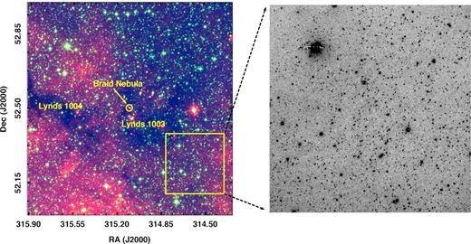
Left-hand panel: IR view (red: WISE W3, green: WISE W1, blue: 2MASS Ks) of dark cloud Lynds 1003 and Lynds 1004 towards Cyg OB7 region. The braid nebula is also marked. Our optical FOV is marked in yellow square. Right-hand panel: Optical I-band image of our studied region (yellow square in the left-hand panel) was observed using 1.3m DFOT. See the text for details.
Identification of variable candidates needs long-term monitoring over a large number of stars. Such investigation involved not only for characterizing variability but also for detecting interesting and rare objects with their rare phenomena. The principal focus of the SFR monitoring is related to many questions as the fraction of young stars that exhibit variability, the amplitude and rotation period of photometric fluctuation, and dominant physical mechanisms related to it. In this contribution, we present here opticalItime-series photometry over an area ∼15 arcmin × 15 arcmin centred on α2000 = 20h58m28s δ2000 = +52015m26s towards south-western outskirts of Lynds 1003 cloud in Cyg OB7, overlapping with some area monitored by Rice et al. (2012) and Wolk et al. (2013b) in the NIR. The field of view (FOV) of our studied region is displayed in the right-hand panel of Fig. 1. Section 2 describes the data set obtained for this study and the data reduction procedure. Section 3 deals with the identification of variable stars from their time-series photometry and the different types of the observed variability. In Section 4, we discuss the characteristics of the candidate variables including the possible correlation between variability and circumstellar disc material, and the spatial distribution of variable stars in the molecular clouds. Our conclusions are summarized in Section 5.
2 DATA SETS
2.1 Observations and data processing
Photometric V, R, and I observations were carried out on 17 nights spanning over 1.5 yr during 2014–2015 with three different telescopes. The I-band data were used for monitoring variability.
We performed observations using the 2K × 2K CCD camera on the 1.3 m Devasthal Fast Optical Telescope (DFOT), ARIES, Nainital, India. The FOV of the camera was ∼18 arcmin × 18 arcmin with a plate scale of 0.535 arcsec pixel−1. More detailed on instrument specification and observations technique are described in Dutta et al. (2018a). We carried out further I-band monitoring observations using the 2K × 2K CCD camera of the HFOSC instrument at the 2 m Himalayan Chandra Telescope (HCT), India, which has an FOV ∼10 arcmin × 10 arcmin with a pixel scale of 0.296 arcsec pixel−1 (see Dutta et al. 2018a for details). We observed another set of I-band monitoring observations at the 1.04 m Sampurnanand Telescope (ST) operated by ARIES. The 2K × 2K CCD camera has an FOV about 13 arcmin × 13 arcmin with a plate scale of 0.37 arcsec pixel−1 (see Dutta et al. 2015 for more details).
All the targets and comparison stars were chosen within the linear response curve of the CCD camera for our differential (relative) photometry, for which the observations were taken in both long and short exposures. Thus, we achieved good dynamic coverage of the bright as well as faint sources. We always prefer dark to grey nights for our observations. The sky was clear in most cases and the target field was always far from the Moon during observing nights. The 2 × 2 binning mode was applied during observations to get a better signal-to-noise ratio (SNR). The typical full width at half-maximum (FWHM) of the stars were in the range of 1.0–2.5 arcsec during our whole observing span. We provide the log of observations in Table 1, which includes the date of observations at different telescopes; the number of frames with different exposures in different filters; the average seeing at each night.
Log of observations.
| Date of | Telescope | I | R | V | Avg. seeing |
|---|---|---|---|---|---|
| observations | Exp.(s)× N | Exp.(s)×N | Exp.(s)× N | (arcsec) | |
| 31.03.2014 | 1.3 m DFOT | 120 × 22, 60 × 1 | 250 × 2, 150 × 1 | 300 × 1, 100 × 1 | 1.8 |
| 13.11.2014 | 1.3 m DFOT | 150 × 42, 90 × 20, 60 × 25 | – | – | 1.8 |
| 14.11.2014 | 1.3 m DFOT | 150 × 15, 90 × 1, 60 × 8 | – | – | 1.8 |
| 29.11.2014 | 1.3 m DFOT | 150 × 4, 90 × 3, 30 × 3 | – | – | 2.2 |
| 10.12.2014 | 1.3 m DFOT | 150 × 13, 90 × 10, 20 × 5 | – | – | 1.8 |
| 11.12.2014 | 1.3 m DFOT | 150 × 7, 60 × 5, 20 × 6 | – | – | 1.8 |
| 21.05.2014 | 2.0 m HCT | 120 × 21 | – | – | 2.2 |
| 19.08.2014 | 2.0 m HCT | 120 × 10, 90 × 6, 60 × 8 | – | – | 1.0 |
| 29.10.2014 | 2.0 m HCT | 120 × 3, 90 × 3, 60 × 5 | – | – | 2.5 |
| 30.10.2014 | 2.0 m HCT | 120 × 5, 60 × 3 | – | – | 2.5 |
| 05.10.2015 | 2.0 m HCT | 300 × 2, 150 × 4 | 300 × 1, 60 × 1, 10 × 1 | – | 2.5 |
| 06.10.2015 | 2.0 m HCT | 300 × 2, 150 × 4, 60 × 4 | 300 × 1, 30 × 1 | – | 2.5 |
| 07.10.2015 | 2.0 m HCT | 300 × 2, 150 × 3, 60 × 2 | 300 × 1, 30 × 2 | – | 2.5 |
| 28.05.2014 | 1.04 m ST | 150 × 12, 90 × 3, 30 × 2 | – | – | 2.5 |
| 29.05.2014 | 1.04 m ST | 150 × 26 | – | – | 2.5 |
| 03.06.2014 | 1.04 m ST | 150 × 18, 30 × 3 | 200 × 1, 90 × 1 | 250 × 1 | 2.5 |
| 05.06.2014 | 1.04 m ST | 200 × 5, 150 × 31, 60 × 4 | – | – | 2.5 |
The prepossessing of raw images were performed with standard reduction steps in iraf1 software. The image frames were cleaned following bias subtraction, flat-fielding and cosmic ray removal using default tasks available in noao.imred. The point sources were identified with the daofind task of daophot package. The photometry was calculated by point source function (PSF) fitting using allstar task of daophot package (Stetson 1992).
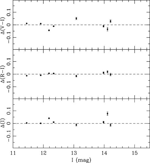
The standardization residuals between transformed and standard magnitudes and colours of observed standard stars are displayed. The combined error bars were propagated from the errors of transformed magnitudes and Landolt (1992).
Finally, we estimated optical magnitudes of the 7009 objects detected in both R and I bands. The I-band light curves of those detected stars were generated from 381 imaging frames using 17-night photometric observations on different telescopes. Nevertheless, we considered 1900 stars for variability studies having at least 140 data points in the overlapping region of three telescopes (Table 1). The completeness limits at various bands were estimated from the histogram turnover method (e.g. Dutta et al. 2015). Our photometric data are complete down to V = 21 mag, R = 21 mag, I = 20.5 mag.
The usage of multiple telescopes makes scaling an issue since the colour transformation varies from the telescope to telescope. So the differential photometry has an added systematic term (magnitude offset). Additionally, the variable stars could have colour variation. Thus, a single set of transformation equation is not sufficient to convert time-series instrumental magnitudes into their standard form. So, we prefer instrument magnitudes for further estimation of variability characteristics. Such systematic variation between two different telescopes could be further reduced by the offset of magnitudes for a set secondary standard star (a list of non-variable stars; see also Section 3.1) observed with those different telescopes. We have considered DFOT magnitudes as primary (since the most number of observations) and applied the estimated offsets for the other two telescopes (HCT and ST). However, if we till accept that there is a significant effect of the colour term in the investigation of variable stars, less than 5 per cent of our sample will have contaminated light curves.
The world coordinate system (WCS) coordinates of the observed stars were estimated using iraf tasks ccmap and ccsetwcs. We selected the positions of 25 isolated moderately bright stars from the Two Micron All Sky Survey (2MASS) point source catalogue (Cutri et al. 2003) to obtain the astrometric solution, which allow us to achieve very good positional accuracy (<0.5 arcsec).
2.2 Archival data set
The NIR observations towards Cyg OB7 (centred on α2000 = |$20^{\rm h}58^{\rm m}28^{s}$| δ2000 = +|$52{^\circ }15{^{\prime}}26{^{\prime\prime}_{.}}0$|) were obtained in JHK bands from the UKIRT Infrared Deep Sky Survey (UKIDSS) data archive observed using WFCAM camera of the 3.8 m UKIRT telescope. In this survey telescope, each pixel corresponds to 0.3 arcsec and yields an FOV ∼20 arcmin × 20 arcmin. The average FWHM during the observing period was ∼1.2 arcsec. The identification of point sources and photometry were performed using iraf with the same procedure described in Section 2.1.
To avoid the inclusion of UKIRT saturated sources, we replaced all the sources in our catalogue having 2MASS magnitudes less than J = 13.25, H = 12.75 and K = 12.0 mag, respectively (Lucas et al. 2008). The magnitude of the sources with uncertainty ≤0.1 mag was taken for our study to ensure good photometric accuracy.
The Wide-field Infrared Survey Explorer (WISE) survey provides photometry at four wavelengths 3.4 (W1), 4.6 (W2), 12 (W3), and 22 (W4) |$\mu$|m, with an angular resolution of 6.1, 6.4, 6.5, 12.0 arcsec, respectively (Cutri & et al. 2012). We used WISE photometric catalog with good-quality photometry (uncertainty better than 20 per cent) in this study.
The Planck satellite observed the entire sky in nine frequency wavebands during 2009-2013 (Planck Collaboration I 2011; Planck Collaboration XXXI 2016) with two instruments: the high-frequency instrument (857, 545, 353, 217, 143, and 100 GHz; Lamarre et al. 2010) and the low-frequency instrument. For this analysis, we used the 857 GHz (350 |$\mu$|m) map.
3 ANALYSIS
3.1 Relative photometry
We selected here five such reference stars for our analysis to produce a set of five independent light curves for each target star, which helped us to cross-verify and rule out any possible contamination from reference stars. An example light curve is shown in Fig. 3 to illustrate the cadence of the data, where we have estimated a mean instrumental magnitude of Iinst = 18.93 mag with an rms = 0.05 mag for the star ID 6828. The errors within a night have an rms of about 0.015 for ID6828, which would also vary from star to star for different magnitude range. The intra-night precision is 18 mmag for this example light curves. On the average, the intra-night precision vary as 5 mmag for Iinst = 15 mag; 20 mmag Iinst = 19 mag; 70 mmag for Iinst = 22.5 mag; thus, we achieve very good photometric precision in our overall observed data points even in the high nebulous and crowded region. The mean intra-night error of magnitudes is 0.019. Finally, after folding all 17-night data, we estimated an rms of magnitudes of about 50 mmag for the above example.
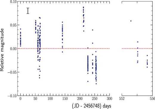
The observed light curve is shown for the ID6828 of mean Iinst = 18.93 mag (Istd = 17.05 mag) with an rms = 0.05 mag. The rms of all photometric precision (= 0.015 mag) is also marked in top-left corner (see the text for details).
3.2 Selection of variable candidates
The identification of variable stars was performed by means of careful inspection of the light curves. First, we estimated rms (σmag) deviation of relative magnitudes for all the stars (e.g. Dutta et al. 2018a). In the Fig. 4, the lower envelope represents an expected trend of σmag as a function of stellar brightness, where σmag increases with Iinst magnitudes since SNR decreases accordingly. The σmag values range from ∼0.013 mag for the bright stars to ∼0.12 mag for stars towards completeness limit (see Section 2.1). Eventually, a few of them are scattered from the normal trend. These scattered outliers may arise from several facts, e.g. intrinsic variability of the star itself, photometric noise, and variation in sky signal. Moreover, visual inspection of observed light curves (Section 3.1) indicated that a few stars show large rms scatter because of abrupt flux change of only a few data points. None the less, such spurious measurements were rejected as their false variability comes from their location on the edge of CCD, the effect of the bad pixel or cosmic ray hits.
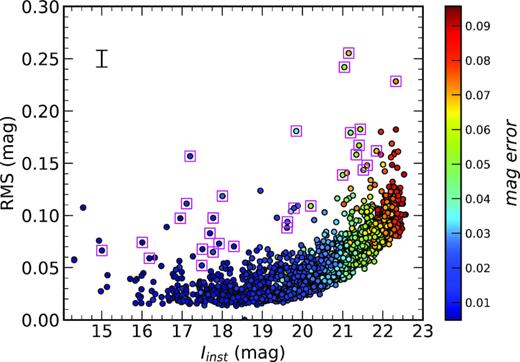
RMS distribution of the Iinst magnitudes of 1900 stars towards Cyg OB7 is shown. The magenta boxes are the candidate variables identified from their observed light curves. An average value of error in rms is plotted in the top left corner. The colour bar indicates the average magnitude error associated with each magnitude (see the text for details).
The candidate variables were selected from the observed 1900 light curves based on 3σ rms scatter from the mean in each magnitude bin (see Fig. 4). From Fig. 4, it is clear that all the candidate variables are lying above ∼0.01 mag from the ‘banana’-shaped pattern of non-variable stars; however, the variables were further authenticated with their observed light curves by visual inspection. Finally, we identified a total of 31 variable stars from the light-curve analyses. A few observed light curves of variable stars are shown in Fig. 5 for four-night observations, to reflect our confidence of visual inspection during variable selection. The average error bar corresponding to each star is displayed. The ‘GAP’3 represents the absence of data points on that night. The catalogue of variable stars and their light-curve analysis are presented in Tables 2 and 3, respectively.
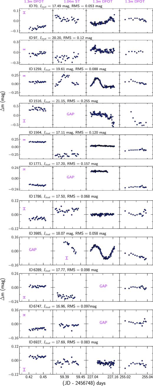
A few examples of differential light curves are plotted. The telescopes of each dataset are marked on top of each panel. The average error bar (in magenta) for each star is shown in the first panel for each row. The ‘GAP’ indicates the absence of data points on that night (see the text for details).
Catalogue of the identified variable stars.a
| ID | RA (J2000) | Dec. (J2000) | V − I | R − I | I | J | H | K | W1 | W2 | W3 | W4 |
|---|---|---|---|---|---|---|---|---|---|---|---|---|
| (hh:mm:ss) | (dd:mm:ss) | (mag) | (mag) | (mag) | (mag) | (mag) | (mag) | (mag) | (mag) | (mag) | (mag) | |
| 8 | 20:57:59.76 | + 52:13:01.74 | – | 1.091 | 19.887 | 16.543 | 15.830 | 15.480 | – | – | – | – |
| – | ± 0.074 | ± 0.036 | ± 0.010 | ± 0.009 | ± 0.015 | – | – | – | – | |||
| 70 | 20:58:1.56 | + 52:20:9.53 | 2.140 | 0.693 | 15.486 | 13.566 | 13.168 | 12.960 | 12.742 | 12.705 | 12.745 | 9.293 |
| ± 0.167 | ± 0.030 | ± 0.022 | ± 0.001 | ± 0.001 | ± 0.002 | ± 0.036 | ± 0.037 | – | – | |||
| 97 | 20:58:2.64 | + 52:11:59.93 | 2.289 | 0.846 | 18.464 | 16.235 | 15.637 | 15.419 | 14.156 | 14.348 | 12.811 | 9.229 |
| ± 0.105 | ± 0.077 | ± 0.061 | ± 0.008 | ± 0.008 | ± 0.014 | ± 0.025 | ± 0.037 | ± 0.456 | ± 0.425 | |||
| 104 | 20:58:2.64 | + 52:21:20.81 | 1.798 | 0.772 | 16.127 | 14.049 | 13.527 | 13.317 | 11.921 | 11.930 | 11.390 | 9.168 |
| ± 0.045 | ± 0.031 | ± 0.025 | ± 0.002 | ± 0.001 | ± 0.003 | ± 0.022 | ± 0.022 | ± 0.132 | ± 0.426 | |||
| 567 | 20:58:16.68 | + 52:11:11.98 | – | – | 16.331 | 13.065 | 11.937 | 11.582 | 11.268 | 11.318 | 11.500 | 9.347 |
| – | – | ± 0.040 | ± 0.027 | ± 0.027 | ± 0.020 | ± 0.023 | ± 0.021 | ± 0.141 | – | |||
| 750 | 20:58:22.08 | + 52:12:12.10 | – | 1.063 | 18.192 | 15.120 | 14.492 | 14.171 | 13.391 | 13.423 | 11.548 | 9.191 |
| – | ± 0.055 | ± 0.033 | ± 0.003 | ± 0.003 | ± 0.005 | ± 0.028 | ± 0.031 | ± 0.161 | ± 0.497 | |||
| 771 | 20:58:22.44 | + 52:16:25.61 | – | 0.874 | 20.396 | 17.071 | 16.362 | 16.044 | – | – | – | – |
| – | ± 0.070 | ± 0.062 | ± 0.016 | ± 0.014 | ± 0.025 | – | – | – | – | |||
| 832 | 20:58:24.24 | + 52:11:52.04 | 1.663 | 0.740 | 15.877 | 13.843 | 13.422 | 13.193 | 12.447 | 12.462 | 12.377 | 9.181 |
| ± 0.034 | ± 0.034 | ± 0.020 | ± 0.001 | ± 0.001 | ± 0.002 | ± 0.026 | ± 0.027 | ± 0.423 | – | |||
| 954 | 20:58:27.12 | + 52:16:34.43 | – | 1.237 | 21.399 | 17.992 | 17.358 | 17.091 | – | – | – | – |
| – | ± 0.117 | ± 0.080 | ± 0.035 | ± 0.035 | ± 0.064 | – | – | – | – | |||
| 1142 | 20:58:33.96 | + 52:15:41.04 | 1.779 | 0.807 | 16.593 | 14.210 | 13.721 | 13.495 | 12.545 | 12.632 | 12.322 | 9.350 |
| ± 0.043 | ± 0.010 | ± 0.006 | ± 0.002 | ± 0.002 | ± 0.003 | ± 0.024 | ± 0.025 | – | – | |||
| 1170 | 20:58:34.68 | + 52:12:20.77 | – | 1.396 | 19.677 | 16.658 | 15.910 | 15.573 | – | – | – | – |
| – | ± 0.063 | ± 0.056 | ± 0.011 | ± 0.010 | ± 0.016 | – | – | – | – | |||
| 1259 | 20:58:38.28 | + 52:11:50.21 | 1.805 | 0.925 | 18.050 | 15.207 | 14.499 | 14.217 | 13.780 | 13.740 | 12.748 | 9.371 |
| ± 0.117 | ± 0.024 | ± 0.011 | ± 0.004 | ± 0.003 | ± 0.005 | ± 0.026 | ± 0.036 | – | – | |||
| 1269 | 20:58:38.64 | + 52:14:26.30 | 2.379 | 1.071 | 18.394 | 15.483 | 14.842 | 14.497 | 13.104 | 13.090 | 12.661 | 9.407 |
| ± 0.086 | ± 0.056 | ± 0.044 | ± 0.004 | ± 0.004 | ± 0.007 | ± 0.026 | ± 0.030 | – | – | |||
| 1422 | 20:58:43.68 | + 52:13:16.82 | – | 1.122 | 20.288 | 17.143 | 16.324 | 16.062 | – | – | – | – |
| – | ± 0.116 | ± 0.068 | ± 0.017 | ± 0.014 | ± 0.026 | – | – | – | – | |||
| 1509 | 20:58:46.92 | + 52:19:41.88 | – | 0.755 | 19.793 | 17.127 | 16.287 | 15.976 | – | – | – | – |
| – | ± 0.090 | ± 0.053 | ± 0.016 | ± 0.013 | ± 0.023 | – | – | – | – | |||
| 1516 | 20:58:47.64 | + 52:19:4.84 | – | – | 20.504 | 17.361 | 16.468 | 16.144 | – | – | – | – |
| – | – | ± 0.071 | ± 0.020 | ± 0.016 | ± 0.027 | – | – | – | – | |||
| 1549 | 20:58:49.08 | + 52:12:29.41 | – | – | 20.178 | 15.795 | 14.590 | 14.071 | – | – | – | – |
| – | – | ± 0.046 | ± 0.005 | ± 0.003 | ± 0.005 | – | – | – | – | |||
| 1564 | 20:58:49.80 | + 52:19:46.60 | 2.117 | 0.771 | 15.461 | 12.784 | 11.770 | 11.113 | 10.259 | 9.839 | 8.269 | 6.307 |
| ± 0.118 | ± 0.026 | ± 0.011 | ± 0.026 | ± 0.023 | ± 0.024 | ± 0.022 | ± 0.020 | ± 0.023 | ± 0.049 | |||
| 1633 | 20:58:52.32 | + 52:18:0.22 | – | 1.092 | 20.259 | 17.348 | 16.467 | 16.136 | 14.563 | 14.765 | 12.472 | 8.825 |
| – | ± 0.135 | ± 0.089 | ± 0.020 | ± 0.016 | ± 0.029 | ± 0.032 | ± 0.051 | ± 0.358 | – | |||
| 1648 | 20:58:53.04 | + 52:18:44.57 | 1.042 | 0.482 | 13.937 | 12.556 | 12.097 | 11.966 | 11.926 | 12.035 | 12.024 | 9.155 |
| ± 0.017 | ± 0.010 | ± 0.006 | ± 0.017 | ± 0.017 | ± 0.027 | ± 0.022 | ± 0.021 | ± 0.286 | – | |||
| 1751 | 20:58:59.16 | + 52:18:16.78 | 3.677 | 1.581 | 17.310 | 12.273 | 10.972 | 10.486 | 10.122 | 10.141 | 9.904 | 9.401 |
| ± 0.062 | ± 0.012 | ± 0.006 | ± 0.020 | ± 0.017 | ± 0.022 | ± 0.023 | ± 0.021 | ± 0.043 | – | |||
| 1771 | 20:58:59.88 | + 52:22:18.48 | 2.283 | 1.009 | 15.722 | 12.425 | 11.248 | 10.577 | 10.193 | 9.615 | 7.288 | 4.832 |
| ± 0.039 | ± 0.032 | ± 0.013 | ± 0.019 | ± 0.019 | ± 0.020 | ± 0.023 | ± 0.021 | ± 0.021 | ± 0.029 | |||
| 1786 | 20:59:0.24 | + 52:13:6.53 | 3.096 | 1.362 | 16.564 | 12.357 | 11.294 | 10.892 | 10.637 | 10.669 | 10.629 | 8.856 |
| ± 0.026 | ± 0.009 | ± 0.005 | ± 0.022 | ± 0.024 | ± 0.027 | ± 0.028 | ± 0.027 | ± 0.095 | – | |||
| 3451 | 20:57:47.52 | + 52:20:35.77 | – | – | 18.200 | 15.499 | 14.965 | 14.730 | 14.597 | 14.771 | 13.127 | 9.405 |
| – | – | ± 0.080 | ± 0.004 | ± 0.004 | ± 0.008 | ± 0.032 | ± 0.054 | – | – | |||
| 3985 | 20:57:58.32 | + 52:8:13.70 | – | – | 17.069 | 14.022 | 13.383 | 13.165 | 12.767 | 12.819 | 12.635 | 9.262 |
| – | – | ± 0.089 | ± 0.002 | ± 0.001 | ± 0.002 | ± 0.024 | ± 0.025 | – | – | |||
| 6087 | 20:58:18.48 | + 52:10:18.34 | – | – | 20.367 | 17.224 | 16.449 | 16.084 | – | – | – | – |
| – | – | ± 0.076 | ± 0.018 | ± 0.016 | ± 0.025 | – | – | – | – | |||
| 6289 | 20:59:11.04 | + 52:11:51.00 | 1.830 | 0.868 | 16.030 | 13.724 | 13.269 | 13.053 | 10.829 | 10.830 | 11.088 | 9.355 |
| ± 0.022 | ± 0.020 | ± 0.019 | ± 0.001 | ± 0.001 | ± 0.002 | ± 0.023 | ± 0.021 | ± 0.116 | – | |||
| 6506 | 20:58:55.20 | + 52:13:34.75 | – | 1.304 | 19.935 | 16.363 | 15.563 | 15.163 | 13.429 | 13.473 | 11.947 | 9.001 |
| – | ± 0.098 | ± 0.051 | ± 0.009 | ± 0.007 | ± 0.012 | ± 0.024 | ± 0.029 | ± 0.193 | – | |||
| 6666 | 20:59:10.68 | + 52:15:20.10 | 2.004 | 0.989 | 14.439 | 11.558 | 11.015 | 10.741 | 10.591 | 10.519 | 10.637 | 8.828 |
| ± 0.021 | ± 0.006 | ± 0.006 | ± 0.015 | ± 0.015 | ± 0.022 | ± 0.022 | ± 0.021 | ± 0.077 | – | |||
| 6747 | 20:59:2.76 | + 52:16:27.98 | 3.242 | 1.442 | 16.077 | 11.715 | 10.871 | 10.446 | 10.371 | 10.136 | 10.347 | 9.434 |
| ± 0.054 | ± 0.007 | ± 0.004 | ± 0.015 | ± 0.015 | ± 0.022 | ± 0.022 | ± 0.020 | ± 0.061 | ± 0.532 | |||
| 6927 | 20:59:0.60 | + 52:18:41.22 | 3.156 | 1.390 | 16.760 | 12.388 | 11.329 | 10.912 | 10.514 | 10.514 | 10.319 | 8.711 |
| ± 0.031 | ± 0.012 | ± 0.008 | ± 0.023 | ± 0.026 | ± 0.032 | ± 0.022 | ± 0.020 | ± 0.066 | – |
aThe optical and NIR magnitudes with error < 0.1 mag and WISE magnitudes with error < 0.2 mag were used for this analyses. The magnitudes with null error information were not considered in this study.
Details of the variable stars.
| ID | Imean | rms | Period | FAP | Amp | Spectral Index | Chisq | Agea | Massa | Remarks |
|---|---|---|---|---|---|---|---|---|---|---|
| (mag) | (mag) | (d) | (mag) | (α) | (Myr) | (M|$\odot$|) | ||||
| 8 | 19.89 | 0.186 | 6.67 | <0.01 | 0.41 | – | – | – | – | δ-scuti |
| 70 | 15.49 | 0.044 | 0.28 | <0.01 | 0.05 | – | – | – | – | EB |
| 97 | 18.46 | 0.111 | – | – | – | – | – | – | – | – |
| 104 | 16.13 | 0.050 | – | – | – | −1.92 | 0.92 | – | – | MS/Field |
| 567 | 16.33 | 0.125 | – | – | – | −2.84 | 0.99 | – | – | MS/Field |
| 750 | 18.19 | 0.10 | – | – | – | −1.41 | 0.95 | – | – | CTTS |
| 771 | 20.40 | 0.18 | – | – | – | – | – | – | – | – |
| 832 | 15.88 | 0.07 | – | – | – | – | – | – | – | – |
| 954 | 21.40 | 0.23 | 0.43 | <0.01 | 0.27 | – | – | – | – | – |
| 1142 | 16.59 | 0.07 | – | – | – | – | – | – | – | – |
| 1170 | 19.68 | 0.14 | 11.58 | <0.01 | 0.35 | – | – | – | – | δ-scuti |
| 1259 | 18.05 | 0.09 | 0.30 | <0.01 | 0.20 | – | – | – | – | Ex-Lupi |
| 1269 | 18.39 | 0.19 | 2.40 | <0.01 | 0.16 | – | – | – | – | – |
| 1422 | 20.29 | 0.15 | – | – | – | – | – | – | – | – |
| 1509 | 19.79 | 0.17 | – | – | – | – | – | – | – | – |
| 1516 | 20.50 | 0.26 | 0.58 | <0.01 | 0.62 | – | – | – | – | – |
| 1549 | 20.18 | 0.16 | – | – | – | – | – | – | – | – |
| 1564 | 15.46 | 0.11 | 5.17 | <0.01 | 0.31 | −1.01 | 0.94 | 5.12 ± 0.88 | 0.80 ± 0.03 | CTTS |
| 1633 | 20.26 | 0.15 | 9.87 | <0.01 | 0.19 | – | – | – | – | – |
| 1648 | 13.94 | 0.05 | – | – | – | – | – | – | – | – |
| 1751 | 17.31 | 0.07 | – | – | – | −2.55 | 0.99 | 1.82 ± 0.51 | 0.13 ± 0.02 | MS/Field |
| 1771 | 15.72 | 0.16 | – | – | – | −0.31 | 0.90 | 4.46 ± 1.12 | 0.67 ± 0.04 | CTTS |
| 1786 | 16.56 | 0.06 | – | – | – | −2.73 | 0.99 | 3.97 ± 0.76 | 0.24 ± 0.02 | MS/Field |
| 3451 | 18.20 | 0.10 | – | – | – | – | – | – | – | – |
| 3985 | 17.07 | 0.05 | 0.15 | <0.01 | 0.15 | −2.40 | 0.99 | – | – | MS/Field; EB |
| 6087 | 20.37 | 0.16 | – | – | – | – | – | – | – | – |
| 6289 | 16.03 | 0.11 | 1.70 | <0.01 | 0.18 | −2.03 | 0.75 | – | – | MS/Field; EB |
| 6506 | 19.93 | 0.25 | 1.18 | <0.01 | 0.72 | −1.21 | 0.80 | – | – | CTTS |
| 6666 | 14.44 | 0.07 | 2.44 | <0.01 | 0.09 | −2.80 | 0.99 | 2.22 ± 0.29 | 0.70 ± 0.04 | MS/Field; EB |
| 6747 | 16.08 | 0.09 | 1.58 | <0.01 | 0.09 | −2.79 | 0.99 | 2.25 ± 0.75 | 0.23 ± 0.02 | MS/Field; EB |
| 6927 | 16.76 | 0.07 | – | – | – | −2.33 | 0.99 | 3.03 ± 0.34 | 0.20 ± 0.03 | MS/Field |
aAge and Mass are estimated from V/V − I colour–magnitude diagram.
3.3 Period estimation
We searched for the periodic signals in all of the monitored stars independent of their observed light curve and σmag deviation. We made use of the Lomb–Scargle (LS) periodogram analysis technique (Lomb 1976; Scargle 1982). The LS method is used to find out significant periodicity even with unevenly sampled data and was verified successfully in several cases to determine periods from such sparse data sets (e.g. Lamm et al. 2004; Mondal et al. 2010; Lata et al. 2012). This method calculates the normalized power for a given angular frequency and locates the highest peak in the estimated periodogram. This highest peak is considered as the most significant peak [false alarm probability (FAP) < 0.01] and provides the period of the time-series data.
The highest frequency corresponds to the Nyquist frequency, which is measured on the basis of average observational spacing. The periodogram peak could fall in the gap between the chosen grid points of frequency. So, a reliable approach is to use the frequency heuristic to decide on the appropriate grid spacing to use, or passing a minimum and maximum frequency. The minimum frequency corresponds to the time range and the maximum frequency is obtained from the median of consecutive observational spacing. Alternatively, to achieve a more precise estimate of the periods, we chose a very small step size of frequency to smoothly sample the periodogram as we zoom in towards the period. In this approach, the step size of the period search algorithm is a function of the square of the period. We consider a step size of ∼0.001 d for periods less than 3 d and ∼0.015 d for a period up to 12 d. The derived (linear) frequencies has the formal error, δf = 3σN/2TA |$\sqrt{N_0}$| (Horne & Baliunas 1986), where σN is the variance of noise in the period subtracted signal, T is the span of time baseline (∼550 d), A is the signal amplitude (typically 10 per cent), N0 is the number of independent data points (∼300). Thus, we obtain the formal error of the order of ∼0.001 d. We measure the periods nearest to 0.01 d, which is quite reasonable for our period measurements of less than 12 d.
We used the LS algorithm at the starlink4 software package. Our time-series data consist of 17-night sparse data, where each night observations are relatively dense packed. We feed all the points as a single file to the software package, further we verified the small periodic variable with each night observations separately in order to avoid any misinterpretation of such unevenly shaped data sets by the LS code. We note that non-variables are often subjected to 0.5 or 1.0 d periodicity in LS analyses, likely due to ∼1 d separation in our consecutive night observations. Thus, we have rejected certain windows of periods between 0.45–0.55 d and 0.90–1.1 d to avoid the induced aliasing in our data set. Since the LS method favours sinusoidal light curves, it cannot accurately analyse the sharp eclipsing system. However, our variable list does not have many sharp eclipsing systems to draw special attention. The periods were further verified with period045 (Lenz & Breger 2005) and NASA Exoplanet Archive Periodogram Service.6 Fig. 6 displays example LS power spectra of ID70. The estimated periods using the Starlink package are 0.28 d. We estimated the periodicity of 14 stars from our sample, which were all identified as variable from their observed relative photometry light curve. Each observed light curve was folded with the estimated period to generate phase light curve. Fig. 7 shows the mean of differential magnitudes in 0.05 phase bin as a function of phase, where the error bars represent the σ of the mean in each bin. Out of 31, 17 candidate variables were considered as irregular based on their insufficiently convincing phased light curves. The periods of all the stars are listed in Table 3.
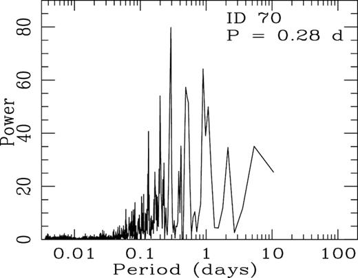
Example LS power spectra of a variable star. The highest peaks correspond to the period of the star.
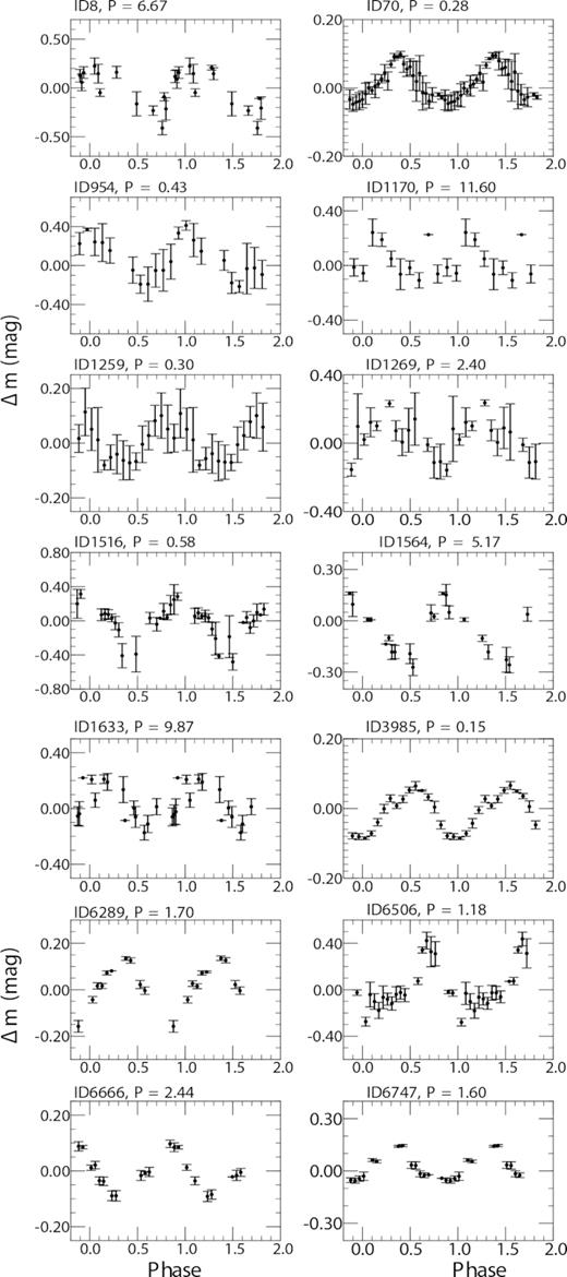
Phase light curves of periodic variables (see the text for details).
3.4 Previously known variables
Rice et al. (2012) and Wolk et al. (2013a) detected many variable stars including disc-bearing young stars using the J, H, K monitoring of the dark clouds Lynds 1003/1004 in the Cyg OB7. Our observing FOV coincides with a part of their coverage. From the list of the variables in Rice et al. (2012) only two (RWA 4 or ID 1771 and RWA 16 or ID 1564) were measured in our field and bright enough to analyse. Since RWA stars were measured in JHK and most are somewhat obscured, hence they were too faint in I band. The variability of those RWA 4 and RWA 16 was confirmed. Rice et al. (2012) found ID 1564 and ID 1771 as periodic variables with periodicity 4.84 and 6.35 d, respectively. Our present data suggest a period of 5.17 d for ID1564, whereas ID1771 is aperiodic. Similarly, Out of 13 variable stars identified by Wolk et al. (2013a) from NIR JHK photometry in this direction of Cygnus OB7, the star ID 70 is studied and found as a variable in the present analyses. We estimated a period of 0.28 d for ID 70 (RAJ2000 = |$20^{\rm h}58^{\rm m}01{^{\rm s}_{.}}70$|, Dec.J2000 = +|$52{^\circ }20{^{\prime}}09{^{\prime\prime}}$|), which is nicely match with the period (0.30 d; an eclipsing system) measured by Wolk et al. (2013a). ID 1648 and ID 6666 are listed in the American Association of Variable Star Observers (AAVSO) data base from Photometric All Sky Survey (APASS) DR9 (Henden et al. 2016).
4 DISCUSSIONS
4.1 PMS variable stars
Photometric variability is a defining characteristic of PMS stars; however, their detection in optical could be limited due to the dominance of circumstellar disc emission in IR. Optical monitoring has been widely used to characterize the PMS variability (e.g. Herbst et al. 2000; Carpenter et al. 2001; Lamm et al. 2004; Makidon et al. 2004; Littlefair et al. 2005; Briceño et al. 2005; Cody et al. 2017; Dutta et al. 2018a). In addition, variability might be a sign of being PMS, but is more often associated with other phenomena, binarity and pulsation related to age. To detect young stars from the variable candidates, we have utilized NIR (J, H, K) and MIR (WISE 3.4, 4.6, 12, and 22 |$\mu$|m).
4.1.1 Spectral energy distribution
The evolutionary stages of the YSOs could be suggested by the spectral energy distribution (SED). We estimated spectral index [α = dlog (λFλ)/dlog (λ)] of the variable sources. Following Lada et al. (2006), objects with α ≥ + 0.3 are considered as Class I, −0.3 ≥ α ≥ +0.3 flat spectrum, −0.3 < α < −1.8 as Class II, and α < −1.8 as Class III sources. Out of 31 variable stars, two have WISE measurements in all four bands. We estimated α for these sources from a least-squares fit to the fluxes in the range of 3.4–24 |$\mu$|m. The α indices of 10 sources are obtained from available K to 12 |$\mu$|m. Other 19 sources are not considered for SED analysis in the present discussion since they do not have longer wavelength coverage, whereas K to 4.6 |$\mu$|m have very little leverage and are very susceptible to the reddening in comparison with K to 12 |$\mu$|m and 3.4–24 |$\mu$|m. All the 12 estimated α indices are listed in Table 3. Using the above approach, we find that four variables (ID750, ID1564, ID1771, and ID 6506) have α > −1.8, which are probable CTTSs. Other eight are either WTTS/Class III, main-sequence (MS) or other field stars. Since, there is no well-defined boundary between WTTSs and field stars, based on SED analyses we could not classify them. We consider the remaining unexplored 19 variables as field stars or discless PMS stars. However, high-resolution multiwavelength spectroscopic observations could further narrow down such classification (Hillenbrand 1997; Luhman 2004; Rice et al. 2012; Herczeg & Hillenbrand 2014; Dutta et al. 2015).
4.1.2 NIR colour–colour and colour–magnitude diagrams
The NIR colour–colour (CC) diagram is shown in Fig. 8 for all the identified candidate variable stars. The locus of dwarfs (solid black line) and giants (long dashed golden line) are adopted from Bessell & Brett (1988). The long dashed red line represents the linear fitting of observed CTTSs by Meyer, Calvet & Hillenbrand (1997). The dotted blue line indicates a reddening vector with slope AJ/AV = 0.265, AH/AV = 0.155, and AK/AV = 0.090 taken from Cohen et al. (1981), a representative reddening vector of AV = 3 mag is also shown in arrow mark. The NIR emission of normal stars is thought to originate from the photosphere and they follow the dwarf locus in NIR CC diagram, whereas their giant counterparts appear more luminous. Nevertheless, the NIR emission of CTTSs is dominated by the circumstellar disc in addition to photospheric emission (Lada & Adams 1992). Thus, they advance according to the reddening vector based on the amount of emission coming from the circumstellar material.
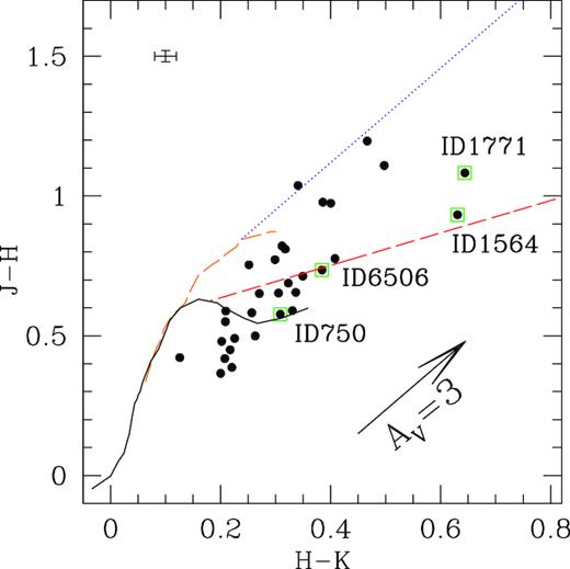
The J − H/H − K CC diagram of candidate variable stars in Cyg OB7. The green boxes represent the location of the probable CTTSs identified using α indices. The locus for dwarfs (solid black) and giants (long dashed golden line) are taken from Bessell & Brett (1988). The long dashed red line represents the CTTSs locus from Meyer et al. (1997). Average error bars are shown in the left top corner. The dotted blue line is the reddening vector taken from Cohen et al. (1981). The reddening vector of visual extinction AV = 3 mag is also marked (see the text for details).
Objects ID1564 and 1771 are both absorbed by over AV = 3 mag of extinction in Fig. 8. Additionally, from our SED analyses, we also find that ID740 and ID 6506 are CTTSs. All CTTSs are marked with the green boxes in Fig. 8. The remaining 27 are either field stars or discless PMS/Class III stars. Naturally, Class III sources are very difficult to distinguish from the field stars based on NIR excess. We suggest further high-resolution spectroscopic observations to evaluate physically each of the sources.
The stars ID1564 and ID1771 also show strong H α emission (equivalent width > 10 Å) in (r − i)/(r − H α) CC diagram (figures are not shown) based on IPHAS photometry (e.g. Barentsen et al. 2011; Dutta et al. 2018a).
The J versus (J − H) colour–magnitude diagram (CMD) is another important tool to get the approximate knowledge about masses of the PMSs, since they are more easily detectable over more extinct optical (e.g. V versus V − I) wavelengths from the molecular cloud. Furthermore, the longer wavelengths (e.g. K versus H − K) CMD might be contaminated by circumstellar extinction. In Fig. 9, the candidate variables are compared with mass bins of representative ages 2 and 5 Myr. Notably, the location of PMSs moves along the reddening vector from the theoretical isochrones depending upon circumstellar disc emission. Two PMS variables (ID1564 and ID1771) seem to confine between 2.6 and 1.0 M|$\odot$|; another two (ID750 and ID6506) appear to be low-mass stars (∼0.1 M|$\odot$|). Since we have used PMS isochrone in these analyses, we could not predict the mass range of non-PMS stars.
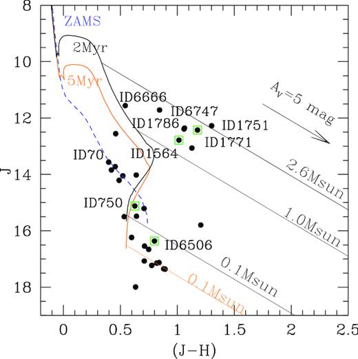
The J/(J − H) CMD for all the candidate variable stars. The green boxes are the CTTSs, the identification is marked. All the stars with age < 5 Myr (see Fig. 10) are also marked. The blue curve indicates the ZAMS. Two representative ages 2 and 5 Myr are shown in black and yellow, respectively. Different reddening vectors are drawn from 2.6, 1.0, 0.1 M|$\odot$| mass for different ages. All the isochrones and tracks are corrected for the distance. A representative reddening vector of visual extinction AV = 5 mag is also displayed.
This analysis is highly dependent on the age of PMSs, a change between 2 and 5 Myr would result in 30–50 per cent agreement of the present mass estimation. Such mass estimation could also be affected by several errors such as the variable nature of stars, the presence of EB, and emission from the circumstellar material.
4.1.3 Optical CMD
The observed VI photometry was employed to estimate the approximate ages and masses of PMS candidate variables. The V versus (V − I) CMD is displayed in Fig. 10, where zero-age main sequence (ZAMS) from Girardi et al. (2002) is represented by dotted black curve. Different theoretical PMS isochrones (Siess, Dufour & Forestini 2000; Bressan et al. 2012) for ages of 1, 5, and 10 Myr are shown as the nearly vertical lines. The solid black curves are evolutionary mass tracks for different mass bins from Siess et al. (2000). All the theoretical models are corrected for cluster distance 760 pc.7 The background stars are fitted well with a reddening of E(B − V) = 0.30 mag, which is considered as background extinction of the studied region. This background reddening value in optical is also consistent with the single epoch UKIDSS (NIR) data.
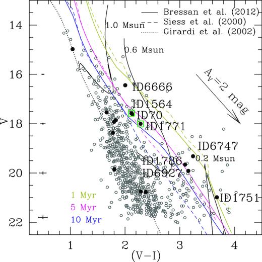
The V/(V − I) CMD for all the sources of the studied region. The black circles are the candidate variable sources, whereas green boxes are CTTSs (the identification are marked). The identification of the stars with age <5 Myr is also marked. The dotted curve is the locus of ZAMS from Girardi et al. (2002); solid curves are the PMS isochrones of age 1.0, 5.0, and 10.0 Myr, respectively; and the thin black solid curves are the evolutionary tracks for various mass bins from Siess et al. (2000). The long dashed curves are PMS isochrones of age 1.0, 5.0, and 10.0 Myr taken from Siess et al. (2000). All the isochrones and tracks are corrected for the distance and reddening. Average error bars are shown on the left-hand side. The reddening vector of visual extinction AV = 2 mag is shown.
We estimated the masses and ages of a few PMS candidate variable stars using interpolation methods of Siess et al. (2000) isochrones in the CMD. The estimated ages and masses are listed in Table 3. Out of 31, 15 variables have V-band detection (black circles in Fig. 10). The CMD positions of ID1564 and ID1771 CTTS variables seem to be adequately fit for ∼5 Myr; another six sources have age less than 5 Myr. Although, different models at the low-mass end differ significantly as we can see in Fig. 10. The masses of the variables seem to be in the range of 0.2–1.0 M⊙. Notably, eight sources are located along ZAMS. Since we are using PMSs isochrone in these analyses, the stars located around ZAMS are not considered for mass and age estimation in the above approach. The reddening vector is nearly parallel to the isochrones; a small extinction variation would not have much effect on the age estimation of variable stars. However, such measurement will lead to 50–60 per cent error in case of unresolved binary. The presence of binary will brighten a star from its actual measurement; hence, a lower age estimation is predicted. None the less, the average age of young stars is deduced 1–2 Myr (e.g. Gutermuth et al. 2009). The extinction from the natal molecular environment and circumstellar envelope around YSOs could introduce over local background subtraction during photometry, which could lead to an apparent age spread up to ∼10 Myr in optical CMD.
4.2 Other variables: eclipsing binaries
As discussed earlier 13 per cent (4 out of 31) variables are PMS. The rest are field stars, with some discless PMS stars. We have estimated the periodicity of 45 per cent (14 out of 31) variable candidates. Remaining 55 per cent are considered stochastic sources; however, only two (ID1771 and ID750) among them have IR excess. The variable stars could be classified based on the shape of their phase and observed light curves. Note that we do not attempt to classify the light curves by the physical characteristics of the stars due to the lack of sufficient data.
Eclipsing binaries are easiest detectable variable stars due to their smooth, stable periodic light curves, prominent sudden drop on their magnitudes. The smooth phase light curves of five sources (ID70, ID3985, ID6289, ID6666, ID6747) indicate that they are an eclipsing system. The star ID70 was earlier detected as W UMa (or WMa) EB system with a short period (0.30 d) by Wolk et al. (2013a). Short periods and smooth observed light-curve pattern of ID3985 are also similar to WMa objects. This type of EB variable is known as a low-mass contact binary of stars with spectral type G or K. The stars ID8, ID1170, ID6506 are suspected to be δ-scuti. ID1259 is probably a young eruptive variable of type Ex-Lupi; however, we do not find any signature of IR excess around it in this analyses (see also Section 4.1.1).
4.2.1 Correlation between photometric variability and circumstellar discs
Since circumstellar discs play a vital role in PMS variability (e.g. Edwards et al. 1993; Herbst et al. 2002; Nordhagen et al. 2006; Dutta et al. 2018a), we looked for any possible correlation between NIR excess and rotation. Fig. 11 displays spectral index against rotation period. While the number of stars is too small to provide a good statistical significance, the general form of the distribution is quite similar to what is seen in the ONC (Herbst et al. 2002), IC 348 (Nordhagen et al. 2006), or NGC 2282 (e.g. Dutta et al. 2018a). One CTTS star (ID6506) has the period less than 2 d and another CTTS (ID1564) is relatively slow rotators. A small number of rotators in our sample prevents to establish any conclusion, notably, the rapid rotators tend to have less IR excess (larger negative slopes), while the slower rotators should have a mixture of stars with optically thick accretion discs and stars without such discs. More interestingly, all the eclipsing binaries have a small period and large spectral indices. Such large values of alpha indices of binaries, beyond the blackbody (αBB = −1.80), possibly arising from the contamination of photometry by the binary counterpart, which make them more luminous as they are. However, such steeper αBB could also be driven by bad data at the red end.
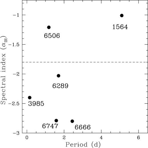
Spectral indices of the candidate variable stars, as defined by Lada et al. (2006), on the basis of their IR data, shown as a function of the rotational period. The dashed line at α = −1.8 represents the separation between probable CTTSs and discless stars. All the star identifications are marked (see the text for details).
4.2.2 Large-scale view of spatial distribution of variables
Fig. 1 (left-hand panel) shows the large-scale structure around dark cloud Lynds 1003/1004 in IR (2MASS K: blue; WISE W1: green; WISE W3: red). The WISE W3 (12 |$\mu$|m) band is affected by the polycyclic aromatic hydrocarbon (PAH) emissions, which are believed to be excited by UV radiation from the massive star(s) and are present at the interface between the H ii and neutral molecular gas. In Fig. 12 (left-hand panel), we displayed the studied region in Planck 857 GHz (350 |$\mu$|m) map. As the high-frequency channels of the third-generation mission, Planck covers the peak thermal emission frequencies of dust colder than 14 K; therefore, Planck images probe the coldest parts of the ISM (Planck Collaboration et al. 2011). Thus,Planck images are very useful to correlate between the PMSs in the SFRs (e.g. Dutta et al. 2018b).
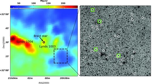
Left-hand panel: Planck 857 GHz map towards the Lynds 1003/1004 molecular clouds. Our studied region is marked with black box. Right-hand panel: Spatial distribution of all the variable sources is over plotted on 2MASS Ks image. Green sources are CTTSs (see the text for details).
In Fig. 12 (right-hand panel), the spatial distribution of candidate variables is shown on 2MASS Ks images. Two PMS stars (ID1564, 1771) are located in the north-eastern direction; these are probably members of Lynds 1003 cloud. Another two PMSs (ID750, 6506) are also along the faint dust ridge in the south-eastern direction.
5 SUMMARY AND CONCLUSIONS
In this paper, we presented I-band time-series photometry of stars towards Cyg OB7 complimented with the optical (V, R, I) observations, archival NIR (J, H, K), WISE (3.4, 4.6, 12, and 22 μm), and Planck (857 GHz) data. We summarized the main results as follows:
The I-band (down to ∼20.5 mag) light-curve analysis enables us to probe the low-mass variable stars, including PMSs. From the photometric light curves, we identified 31 photometric variable stars towards the region. Out of 31, 5 are known from earlier studies, 26 are new variables from this study. The periods of 14 variables are estimated to be in the range of 0.15–11.60 d.
From SED analysis and location on J − H/H − K CC diagram, we selected four variable stars are CTTSs. The remaining stars are unclassified in this study.
The V/(V − I) CMD suggested that variable CTTSs have age <5 Myr and the masses in the range of 0.2–1.0 M⊙.
Five eclipsing systems are identified from the light curves, including one previously known EB.
In the beginning, the goal of this project was to relate IR excess with variability. Unfortunately, a small number of CTTS variables do not represent any obvious correlation. However, we have identified four CTTSs including two previously identified. Photometric monitoring of more number of SFRs would be able to represent a statistically significant correlation between photometric variability and circumstellar disc.
ACKNOWLEDGEMENTS
We are thankful to Dr. Scott Wolk for the valuable comments, which helps us to improve the overall quality of the paper. This work is supported by Satyendra Nath Bose National Centre for Basic Sciences, Kolkata, India under the Department of Science and Technology (DST), Govt. of India. We would like to thank Prof. Wen-Ping Chen for valuable suggestions. This paper made use of the data obtained as part of the United Kingdom Infrared Telescope (UKIRT) Infrared Deep Sky Survey (UKIDSS). This publication also used the data products from the SIMBAD data base (operated at Centre de Donnees astronomiques de Strasbourg (CDS), Strasbourg, France), the Two Micron All-Sky Survey (2MASS), which is a joint project of the University of Massachusetts and the Infrared Processing and Analysis Center/California Institute of Technology, funded by National Aeronautics and Space Administration (NASA) and National Science Foundation (NSF), archival data obtained with the Wide-field Infrared Survey Explorer (WISE) joint project of the University of California, Los Angeles, and the Jet Propulsion Laboratory (JPL), California Institute of Technology (Caltech), funded by the NASA, and the National Optical Astronomy Observatory (NOAO) Science archive, which is operated by the Association of Universities for Research in Astronomy (AURA), Inc., under a cooperative agreement with the National Science Foundation.
Footnotes
Image Reduction and Analysis Facility (iraf) is distributed by National Optical Astronomy Observatories (NOAO), USA (http://iraf.noao.edu/).
We transformed only DFOT instrumental magnitudes to standard magnitudes, since standard magnitudes are utilized for optical CMD only and the DFOT has largest FOV.
Since we have observed with different telescopes with different FOV and also at varying central position to cover all nearby objects in our studied region, a few of the stars may locate at the edge of the CCD, which we remove from further analyses. Moreover, our observations have been carried out with different exposures to achieve good coverage of the bright as well as the faint sources, the total number of points of observations may vary to maintain a good photometric precision for all the data points.
The distance of the region is found to be in the range of 600–800 pc using Gaia DR2, which is also in agreement with this assumed distance.
