


ABSTRACT
We report on the evolution of the X-ray emission of the accreting neutron star (NS) low-mass X-ray binary (LMXB), MXB 1659-298, during its most recent outburst in 2015–17. We detected 60 absorption lines during the soft state (of which 21 at more than 3σ), that disappeared in the hard state (e.g. the Fe xxv and Fe xxvi lines). The absorbing plasma is at rest, likely part of the accretion disc atmosphere. The bulk of the absorption features can be reproduced by a high column density (log (NH/cm−2) ∼ 23.5) of highly ionized (log (ξ/erg cm s−1) ∼ 3.8) plasma. Its disappearance during the hard state is likely the consequence of a thermal photo-ionization instability. MXB 1659-298’s continuum emission can be described by the sum of an absorbed disc blackbody and its Comptonised emission, plus a blackbody component. The observed spectral evolution with state is in line with that typically observed in atoll and stellar mass black hole LMXB. The presence of a relativistic Fe K α disc-line is required during the soft state. We also tentatively detect the Fe xxii doublet, whose ratio suggests an electron density of the absorber of ne > 1013 cm−3, hence, the absorber is likely located at <7 × 10⁴ rg from the illuminating source, well inside the Compton and outer disc radii. MXB 1659-298 is the third well monitored atoll LMXB showcasing intense Fe xxv and Fe xxvi absorption during the soft state that disappears during the hard state.
1 INTRODUCTION
Winds are fundamental components of accretion on to X-ray binaries (Shakura & Sunyaev 1973; Begelman, McKee & Shields 1983). In black hole (BH) X-ray binaries, they are observed to have an equatorial geometry and a strong state dependence (Miller et al. 2006; Neilsen & Lee 2009; Ponti et al. 2012; Neilsen et al. 2018). Winds might even affect the effective viscosity of the accretion disc, as well as the X-ray binary (orbital period) evolution (Ponti et al. 2017; Tetarenko et al. 2018).
Analogously to black hole (BH), accreting neutron star (NS) systems also show ionized absorbers with similar equatorial geometry, similar column densities and ionizations (Ueda et al. 2004; Díaz Trigo et al. 2006; Díaz Trigo & Boirin 2016; Ponti, Muñoz-Darias & Fender 2016). It is still an open question whether the highly ionized absorbers (traced by Fe xxv and Fe xxvi) in NS share the same state dependence as the ones observed in accreting BH. Recent investigations focused on EXO 0748-676 and AX J1745.6-2901, which are two of the atoll NS systems with the best monitoring in the Fe K band, covering both soft and hard states. In both sources it was observed that the highly ionized absorption is stronger during the soft state, while it is undetected during the hard state (Ponti et al. 2014, 2015, 2018). This might suggest that the state-absorption connection is a common property of NS (atoll) sources.
Although the origin of such state-absorption connection is still debated, the results of photo-ionization computations clearly showed that whenever the soft state absorber in X-ray binaries is illuminated by the hard state spectral energy distribution (SED), the plasma becomes unstable (Jimenez-Garate et al. 2001; Chakravorty, Lee & Neilsen 2013; Higginbottom & Proga 2015; Bianchi et al. 2017). As a result of such photo-ionization thermal instability the plasma is prone to change its properties (e.g. condensing, expanding, etc.) and it will likely migrate to other stable solutions (Bianchi et al. 2017).
To further characterize the properties of the absorbers in accreting NS, as well as to further investigate the state-absorption connection in atoll sources, we triggered XMM–Newton, Chandra, and NuSTAR observations during the last (1.5 yr long) outburst of MXB 1659-298, that started in August 2015 (Bahramian, Heinke & Wijnands 2015; Negoro et al. 2015).
MXB 1659-298 is a transient atoll low-mass X-ray binary displaying type-I X-ray bursts, therefore indicating a neutron star primary (Lewin et al. 1976; Galloway et al. 2008). MXB 1659-298 is a high-inclination system (i ∼ 73–78°; Frank et al. 1987; Ponti et al. 2018), showing dipping and eclipsing events, with an orbital period of Porb = 7.1 h (Cominsky & Wood 1984, 1989; Jain et al. 2017; Iaria et al. 2018). The previous outburst of MXB 1659-298 started on 1999 April and lasted for 2.5 yr (Wijnands et al. 2002). During the 1999–2001 outburst, XMM–Newton observed MXB 1659-298 twice, showing clear evidence for Fe xxv and Fe xxvi, as well as lower ionization, absorption lines (Sidoli et al. 2001), however, no Chandra HETG observation was performed, to best detail the properties of the absorber in the Fe K band.
We report here the analysis of the XMM–Newton, Chandra, NuSTAR, and Swift monitoring campaigns of the last outburst of MXB 1659-298.
2 ASSUMPTIONS
All spectral fits were performed using the xspec software package (version 12.7.0; Arnaud 1996). Uncertainties and upper limits are reported at the 90 per cent confidence level for one interesting parameter, unless otherwise stated. Using X-ray bursts, a distance to MXB 1659-298 of 9 ± 2 or 12 ± 3 kpc has been inferred by Galloway et al. (2008) for a hydrogen or helium-rich ignition layer, respectively. We noted that MXB 1659-298 appears in Gaia DR2, however without parallax estimate, hence consistent with the large distance suggested by previous estimates (Gaia Collaboration et al. 2018). All luminosities, blackbody and disc blackbody radii assume that MXB 1659-298 is located at 10 kpc. To derive the disc blackbody inner radius rDBB, we fit the spectrum with the diskbb model in xspec (Mitsuda et al. 1984; Makishima et al. 1986) the normalization of which provides the apparent inner disc radius (RDBB). Following Kubota et al. (1998), we correct the apparent inner disc radius through the equation: rDBB = ξκ2RDBB (where κ = 2 and |$\xi =\sqrt{(3/7)}\times (6/7)^3$|) in order to estimate the real inner disc radius rDBB. We also assume an inclination of the accretion disc of 75° (Frank et al. 1987; Ponti et al. 2018). We adopt a nominal Eddington limit for MXB 1659-298 of LEdd = 2 × 1038 erg s−1 (appropriate for a primary mass of MNS ∼ 1.4 M⊙ and cosmic composition; Lewin, van Paradijs & Taam 1993). We use the χ2 statistics to fit CCD resolution spectra (we group each spectrum to have a minimum of 30 counts in each bin), while we employ Cash statistics (Cash 1979) to fit the high-resolution unbinned ones. We fit the interstellar absorption with the tbabs model in xspec assuming Wilms, Allen & McCray (2000) abundances and Verner et al. (1996) cross-sections.
3 OBSERVATIONS AND DATA REDUCTION
At the beginning of the 2015–17 outburst of MXB 1659-298, we requested a 40 ks XMM–Newton observation, to either discover or rule out the presence of Fe K absorption during the hard state of this source (archival observations only caught the soft state). XMM–Newton observed MXB 1659-298 on 2015-09-26 (obsid 0748391601). All EPIC cameras were in timing mode with the thin filter applied. The data were analysed with the latest version (17.0.0) of the XMM–Newton (Jansen et al. 2001; Strüder et al. 2001; Turner et al. 2001) Science Analysis System sas, applying the most recent (as of 2017 September 20) calibrations. We reduced the data with the standard pipelines (epchain, emchain, and rgsproc for the EPIC-pn, EPIC-MOS, and RGS camera, respectively). Because of the higher effective area, we show EPIC-pn data only, in addition to the RGS. We extracted the EPIC-pn source photons within rawx 20 and 53 (while the background between 2 and 18), pattern< = 4 and flag= = 0.
Following a softening of the X-ray emission, we triggered pre-approved Chandra observations (performed on 2016 April 21) of MXB 1659-298, to detail the ionized absorber properties during the soft state. The Chandra spectra and response matrices have been produced with the chandra_repro task, reducing the width of the default spatial mask to avoid overlap of the HEG and MEG boxes at high energy (E ≥ 7.3 keV).
NuSTAR (Harrison et al. 2013) observed MXB 1659-298 twice during its 2015–17 outburst, on 2015 September 28 (obsid 90101013002), 2 d after the XMM–Newton observation and on 2016 April 21 (90201017002), simultaneous with the Chandra one. The NuSTAR data were reduced with the standard nupipeline scripts v. 0.4.5 (released on 2016-03-30) and the high-level products produced with the nuproducts tool. The source and background photons were extracted from circular regions of 120 arcsec and 180 arcsec radii, respectively, centred on the source and at the corner of the CCD, respectively. Response matrices appropriate for each data set were generated using the standard software. We did not combine modules. Bursts, dips and eclipses have been removed by generating a light curve in xselect with 60 s time binning in the 3–70 keV energy band and cutting all intervals with a count rate outside the persistent value (e.g. 1.7–3.3 and 10–11 ph s−1 for the two observations).
The outburst of MXB 1659-298 was monitored with the Neil Gehrels Swift Observatory, to characterize the long-term evolution of the spectral energy distribution (SED). Full details on the analysis of the Swift data will be presented in a forthcoming paper (Degenaar et al. in preparation). We analysed the Ultraviolet/Optical Telescope (Roming et al. 2005) data obtained on the same day of the XMM–Newton (obsid: 00034002012; filter w1), the first NuSTAR (00081770001; v,b,u,w1,w2,m2) and the Chandra + NuSTAR (00081918001; v,b,u,w1,w2,m2) observations. The various filters employed allowed us to cover a wavelength range of ≃ 1500–8500 Å (Poole et al. 2008). To extract source photons we used a standard aperture of 3 arcmin, whereas for the background we used a source-free region with a radius of 9 arcmin. For each observation/filter, we first combined all image extensions using uvotimsum and then extracted magnitudes and fluxes using uvotsource.
4 TIMING ANALYSIS AND STATE DETERMINATION
To determine the evolution of the state of the source between the various observations, we first extracted light curves in the 3–10 keV energy range, with time bins of 6 ms.1 We computed the fractional rms in the range 0.002–64 Hz for the XMM–Newton and NuSTAR observations. From the XMM–Newton observation we estimated a fractional rms of 21 ± 4 per cent, this value being typical of the hard state (Muñoz-Darias, Motta & Belloni 2011; Muñoz-Darias et al. 2014). In the case of NuSTAR observations, we followed the method described in Bachetti et al. (2015) in order to properly account for dead time effects. Given the poorer statistics (due to the use of the co-spectrum between the light curves of the two modules) only an upper limit to the 0.002-64 Hz fractional rms of <8 per cent can be derived from the second NuSTAR observation, suggesting that MXB 1659-298 was in the soft state at that time. On the other hand, the rms could not be constrained from the first NuSTAR observation.
Fig. 1 shows the XMM–Newton, NuSTAR and Chandra spectra of MXB 1659-298 during the 2015–17 outburst. In agreement with the timing results, the XMM–Newton spectrum (black data) is characterized by a hard power-law shape, confirming that MXB 1659-298 was in the hard state at that time. The first NuSTAR dataset (red and green data), accumulated 2 d after, also shows a very similar hard spectrum, suggestive of a hard state (Fig. 1). On the other hand, during the simultaneous Chandra (dark and light grey) and second NuSTAR (dark and light blue) observations, MXB 1659-298 displays a softer and significantly brighter emission, below 20 keV, while the source emission drops quickly above 20–30 keV. In agreement with the timing results, this indicates that the source was in the soft state during these observations.
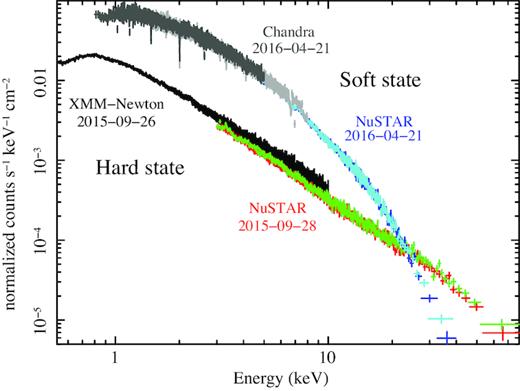
XMM–Newton, NuSTAR, and Chandra spectra of MXB 1659-298 during the 2015–17 outburst. Both the XMM–Newton (black) and NuSTAR (red and green) spectra accumulated on 2015-09-26 and 2015-09-28, respectively, show a hard power law shape characteristic of the hard state. The simultaneous Chandra (light and dark grey) and the NuSTAR (light and dark blue) spectra obtained in 2016-04-21 show a significantly softer and brighter emission below 20 keV, with a significant drop above 20–30 keV.
5 BROAD-BAND FIT OF THE SOFT STATE WITH APPROXIMATE MODELS
We started by simultaneously fitting the Chandra HETG (HEG and MEG first order) + NuSTAR data, leaving the cross-normalization constants (cMEG, cNuA, and cNuB) free to vary (see Fig. 2; Table 1). We fit the MEG, HEG, and FPM(A,B) spectra in the 0.8–6, 1.2–7.3, and 3–45 keV ranges, respectively.
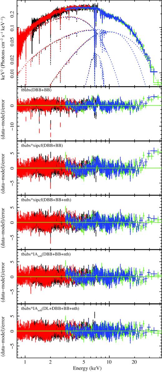
Soft state persistent emission of MXB 1659-298 fitted with phenomenological models. MEG, HEG, FPMA, and FPMB spectra and residuals are shown in red, black, green and blue, respectively. (Top panel) Best fit of the soft state spectrum fitted with disc blackbody plus blackbody plus Comptonization plus a disc-line emission absorbed by neutral and ionized material (Table 1). From top to bottom the various panels show the residuals for increasingly complex models. The first plot shows the residuals of the fit with a disc blackbody plus blackbody model absorbed by neutral material. Then the residuals after the addition of an approximated ionized absorption zxipcf component. Then, residuals after the inclusion of a thermal Comptonization component (nthcomp). Subsequently, residuals after the inclusion of a proper ionized absorption component (IAsoft). Finally, residuals after the inclusion of an additional relativistic Fe K emission line.
Best-fitting parameters of the simultaneous Chandra HETG and NuSTAR spectra. The Chandra HEG and MEG first order as well as NuSTAR FPMA and FPMB spectra (in black, red, green and blue, respectively) are fit simultaneously, leaving a cross-normalization constant free to vary (cMEG, cnuA, and cnuB). The first model, B1, DBB + BB is composed by tbabs(diskbb + bbody), the second, B2, is additionally absorbed by an approximate ionized absorption component (tbabs∗zxipcf(diskbb + bbody)). Model B3 additionally considers the emission from a thermal Comptonization component (tbabs∗zxipcf(diskbb+bbody + nthcomp)). The continuum emission components in model B6 correspond to the ones of B3, however the ionized absorption is substituted by a self consistent one (IAsoft: tbabs∗IA(diskbb+bbody + nthcomp)). Finally, model B7 additionally consider the emission from a relativistic Fe K α line (tbabs∗IA(diskbb+bbody+nthcomp + diskline)). See text for description of the various parameters. ♭ In keV units. ⋆ In units of 1022 cm−2. ‡ Normalization N = R2cos(θ), where R2 is the apparent disc inner disc radius (or blackbody radius) in km, and θ the angle of the disc (θ = 0 face on, cos(θ) = 1 for blackbody).
| Chandra + NuSTARsoft state (2016-04-21) | ||||||
|---|---|---|---|---|---|---|
| Model | B1 | B2 | B3 | B6 | B7 | |
| DBB + BB | xipcf(DBB + BB) | xipcf (DBB+BB + nth) | IA (DBB+BB + nth) | IA (dl+DBB+BB + nth) | ||
| NH | ⋆ | 0.156 ± 0.008 | 0.154 ± 0.009 | 0.229 ± 0.016 | 0.233 ± 0.007 | 0.21 ± 0.01 |
| Log (ξ1) | 4.25 ± 0.02 | 4.25 ± 0.02 | 4.54 ± 0.01 | |$3.76^{+0.12}_{-0.03}$| | ||
| Log |$(N_{H_{1}})$| | ⋆ | 23.6 ± 0.1 | 23.6 ± 0.1 | 24.25 ± 0.02 | |$23.48^{+0.16}_{-0.05}$| | |
| αd | |$-2.61^{+0.07}_{-0.10}$| | |||||
| Nd | × 10−3 | 1.5 ± 0.1 | ||||
| kTDBB | ♭ | 1.62 ± 0.01 | 1.60 ± 0.01 | |$0.89^{+0.04}_{-0.12}$| | 1.02 ± 0.01 | 1.34 ± 0.05 |
| NDBB | ‡ | 5.3 ± 0.1 | 5.6 ± 0.1 | |$6.6^{+0.8}_{-4.0}$| | 8.3 ± 0.1 | 8.7 ± 0.5 |
| kTBB | ♭ | 3.06 ± 0.03 | 2.96 ± 0.03 | 1.23 ± 0.05 | 1.55 ± 0.01 | |$2.51^{+0.05}_{-0.11}$| |
| NBB | ‡ | 0.30 ± 0.01 | 0.37 ± 0.02 | 5.2 ± 1.5 | 1.96 ± 0.05 | 0.43 ± 0.1 |
| kTe | 3.72 ± 0.05 | 3.77 ± 0.02 | |$4.4^{+0.7}_{-0.5}$| | |||
| NComp | × 10−2 | 7.9 ± 1.5 | 6.46 ± 0.04 | |$2.61^{+1.1}_{-0.8}$| | ||
| cMEG | 1.03 ± 0.01 | 1.03 ± 0.01 | 1.03 ± 0.01 | 1.03 ± 0.01 | 1.03 ± 0.01 | |
| cFPMA | 1.00 ± 0.01 | 1.00 ± 0.01 | 1.00 ± 0.01 | 1.00 ± 0.01 | 1.00 ± 0.01 | |
| cFPMB | 1.00 ± 0.01 | 1.00 ± 0.01 | 1.00 ± 0.01 | 1.00 ± 0.01 | 1.00 ± 0.01 | |
| Cstat/dof | 9777.8/7094 | 8133.6/7092 | 7935.7/7090 | 7751.4/7090 | 7584.7/7088 | |
The black, red, green, and blue points in Fig. 2 show the Chandra HEG and MEG, the NuSTAR FPMA and FPMB spectra of the persistent emission, accumulated during the soft state observations (dips, eclipses, and bursts have been removed; see black data in fig. 2 of Ponti et al. 2018). The fit of these spectra with a model composed by a disc blackbody plus a hot blackbody (B1 in Table 1), both absorbed by neutral material (tbabs(diskbb + bbody) in xspec), provided a reasonable description of the continuum, however very significant residuals appeared as clear signatures of ionized absorption lines in the soft X-ray and Fe K band (Fig. 2), making this model unacceptable (C − stat = 9777.8 for 7094 dof, Table 1). We also noted an excess of emission at high energy (E > 25 keV; Fig. 2), that does not appear to be an artefact of the background (contributing at E ≥ 35 keV).
The observed features (see Fig. 2 and Section 6) indicate the presence of ionized absorption. To properly compute the model of the ionized absorption component, the knowledge of the irradiating SED is required. We, therefore, started by first adding an ‘approximated’ ionized absorption component (zxipcf), with the main purpose to initially derive the fiducial SED to be used as input for the photo-ionization computations. After the computation of the proper absorption model the spectra will be re-fitted, obtaining the final best fit.
The addition of an ionized absorption component (B2: tbabs∗zxipcf(diskbb + bbody)) significantly improved the fit (ΔC − stat = 1616.9 for the addition of 2 parameters). The ionized absorption component reasonably reproduced both the soft X-ray absorption lines as well as the strong features in the Fe K band with a large column density (log (NH/cm−2) = 23.6 ± 0.1) of highly ionized material (log (ξ/erg cm s−1) = 4.25 ± 0.02; Table 1). However, highly significant residuals were still present (Fig. 2).
We noted that the excess of emission at energies above E ≥ 25 keV is likely the signature of an additional Comptonization component. We therefore added to the model a thermal inverse-Comptonization component (nthcomp in Xspec). We assumed an asymptotic photon index of Γ = 2 and seed photons produced by the disc blackbody. The fit with this model (B3: tbabs∗zxipcf(diskbb+bbody + nthcomp)) provided a significant improvement of the fit (ΔC − stat = 197.8 for the addition of 2 free parameters; Table 1), properly reproducing the high energy emission (Fig. 2). However, very significant residuals were still present in the 7–10 keV energy range. We noted that part of those residuals might be due to the inaccurate modelling of the ionized absorber. Indeed, the ionized Fe K edges at |$E_{\rm Fe\, {\rm{\small XXV}}}=8.83$| and |$E_{\rm Fe\, {\small XXVI}}=9.28$| keV can contribute to the observed residuals. We, therefore, defer the discussion of such residuals until after the computation of the proper ionized absorber model (see Sections 6.3 and 7).
5.1 Soft state SED
The red solid line in Fig. 3 shows the de-absorbed best-fitting (model B2 of Table 1) soft state SED. The dotted red lines peaking at 3 × 10¹⁷ and 1.5 × 10¹⁸ Hz show the disc blackbody and the blackbody components, respectively. The dashed vertical lines indicate the boundaries where the SED is observationally constrained by the Chandra + NuSTAR data at high energy and by the Swift-UVOT observations (performed in various filters) in the optical–UV band. The observed optical–UV magnitudes range between |$m_{\rm {V_{AB}}}\sim 18$| to |$m_{\rm {UVW2_{AB}}}\sim 20$|. This optical–UV flux is significantly higher than the extrapolated emission from the disc blackbody component dominating in the X-ray band (see Fig. 3). Therefore, this extra flux indicates the presence of an additional component, possibly associated with the irradiated outer disc or the companion star (Hynes et al. 2002; Migliari et al. 2010). We reproduced this emission by adding a blackbody component peaking at 6 × 10¹⁴ Hz (see Fig. 3).
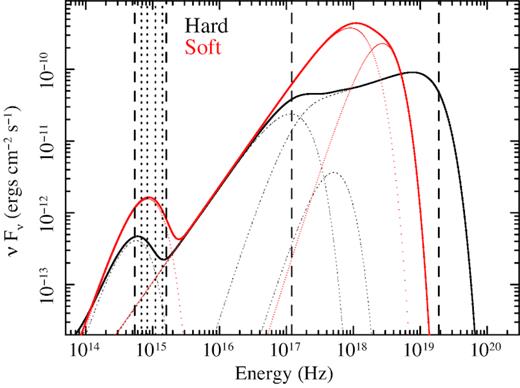
In black and red are shown the de-absorbed best-fitting ‘bona fide’ spectral energy distribution during the hard and soft state, respectively. The dashed lines show the extremes of the X-ray and optical–UV energy ranges constrained by NuSTAR, XMM–Newton, Chandra, and the Swift filters. The dotted vertical lines show the mean energy of the various filters.
We used such bona-fide SED as input for the photo-ionization computations of the absorber that will be presented in Sections 6.3 and 7. Additionally, we tested that considering any of the best-fitting continuum models in Table 1 produced negligible effects on the ionized absorber photo-ionization stability and properties. The photo-ionization computations have been performed with cloudy 17.00 (Ferland et al. 2013).
6 ABSORPTION LINES: Chandra HETG SPECTRUM
We started the characterisation of absorption during the soft state observation, by performing a blind search to hunt for narrow absorption lines in the spectrum of the persistent emission (see Section 9.4 for a discussion of possible caveats). We fitted the Chandra grating data (HEG and MEG are fitted simultaneously) with the best-fitting continuum model reproducing the Chandra + NuSTAR continuum and we added a narrow Gaussian absorption line. We then computed the confidence contours by stepping the energy of the line from E = 0.8 to 9 keV (with 1640 steps logarithmically equally spaced) and the intensity in 10 steps from 0 to −3 × 10⁻⁴ photons cm−2 s−1 in the line. The red, green, and blue contours in Fig. 4 show the 68, 90, and 99 per cent confidence levels. This plot clearly shows the detection of many very significant absorption lines (Fig. 4 and 5).
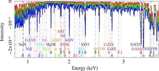
Residuals to the presence of narrow (σ = 1 eV) absorption lines in the Chandra HETG (HEG + MEG) spectra. The red, green, and blue solid lines show the 68, 90, and 99 per cent confidence contours. 60 absorption lines are detected. We highlight with a vertical line each detected absorption feature. The same colour is used for features associated to the same series. In particular, the energies of the α, β, and γ transitions are reported with dashed, dash–dotted, and dotted lines, respectively. Absorption lines associated with Fe L features are highlighted with magenta dot–dot–dot–dashed lines (in violet is the density sensitive Fe xxii doublet). Unidentified lines are shown with grey dotted lines.
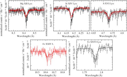
The red and black data display the Chandra HETG MEG and HEG spectra at the energies of some of the strongest lines, respectively, fitted with the best-fitting model (B7 in Table 1). (Top panels) from left to right show the Mg xii Ly α, Si xiv Ly α, and S xvi Ly α lines. The profile of all lines is well reproduced by the best-fitting photo-ionized absorption component. (Bottom panels) from left to right show the two lines of the Fe xxiv L complex and the Fe xxvi Ly α transition. Only data of the MEG and HEG instruments are shown because of their higher effective area at low and high energies, respectively.
To more accurately determine the significance of the detection of the expected absorption features and to measure the equivalent width of the lines, we first divided the spectrum into intervals of 2 Å width and fitted it with the same continuum model (allowing for variations of the normalization). We then added to the model a narrow absorption line with Gaussian profile for each observed residual. We then tested the significance of the residual and we reported in Table 2 all lines detected at more than 90 per cent significance, with associated velocity shifts and equivalent widths. We also highlight with bold characters in Table 2 the lines detected at more than 3σ.
Best-fitting energies (EO), equivalent widths (EW) and outflow velocity (vout) of lines detected in the HETG (HEG + MEG) spectra. For each identified transition the expected wavelength of the transition (λ) is reported. The energies of the doublets are averaged over the oscillator strengths. We only list velocities for the strongest transitions.
| Identification | λ | EO | vout | EW |
|---|---|---|---|---|
| (Å) | (keV) | (km s−1) | (eV) | |
| Fe xviii L | 14.28 | 0.869a | −0.66 ± 0.43 | |
| Ne ix He α (i) | 13.553 | 0.917 ± 0.005 | −0.58 ± 0.47 | |
| Ne ix He α (r) | 13.445 | 0.923 ± 0.007 | −0.56 ± 0.38 | |
| Unid | 0.928 ± 0.006 | −0.57 ± 0.39 | ||
| Unid | |$0.964^{+0.007}_{-0.017}$| | −0.37 ± 0.31 | ||
| Ne x Ly α | 12.133 | 1.0222 ± 0.0004 | −90 ± 120 | −1.72 ± 0.25 |
| Fe xxii L 1σ | 11.92 | |$1.0405^{+0.002}_{-0.009}$| | |$-0.38^{+0.15}_{-0.27}$| | |
| Fe xxii L 1σ | 11.77 | 1.0537 | |$-0.28^{+0.19}_{-0.23}$| | |
| Unid | |$1.094^{+0.007}_{-0.007}$| | −0.36 ± 0.31 | ||
| Fe xvii | 11.018 | 1.120 ± 0.007 | −0.57 ± 0.38 | |
| Fe xxiii | 10.981 | 1.130 ± 0.005 | −0.49 ± 0.34 | |
| Unid | 1.161 ± 0.003 | −0.50 ± 0.39 | ||
| Fe xxiv L | 10.663 | 1.1632 ± 0.0005 | −100 ± 130 | −0.97 ± 0.31 |
| Fe xxiv L | 10.619 | 1.1678 ± 0.00026 | −50 ± 70 | −1.53 ± 0.24 |
| Ne xLy β | 10.239 | 1.211 ± 0.004 | −0.66 ± 0.27 | |
| Na xiLy α | 10.025 | |$1.237^{+0.015}_{-0.007}$| | −0.39 ± 0.22 | |
| Ne x Ly γ | 9.7082 | |$1.277^{+0.004}_{-0.015}$| | −0.26 ± 0.23 | |
| Fe xxi L | 9.356 | |$1.325^{+0.006}_{-0.09}$| | −0.30 ± 0.21 | |
| Mg xi He α? | 9.1688 | |$1.361^{+0.007}_{-0.010}$| | −0.33 ± 0.24 | |
| Fe xxii L | 9.057 | |$1.368^{+0.004}_{-0.009}$| | −0.25 ± 0.18 | |
| Mg xiiLy α | 8.4210 | 1.4728 ± 0.0003 | −100 ± 60 | −2.91 ± 0.21 |
| Fe xxivL | 7.9893 | 1.552 ± 0.002 | −0.38 ± 0.18 | |
| Mg xi He β? | 7.852 | 1.581 ± 0.006 | −0.29 ± 0.23 | |
| Al xii He α | 7.778 | |$1.594^{+0.010}_{-0.018}$| | −0.25 ± 0.20 | |
| Mg xi He γ? | 7.473 | 1.660 ± 0.001 | −180 ± 180 | −0.38 ± 0.23 |
| Mg xi He δ? | 7.310 | 1.695 ± 0.002 | 170 ± 350 | −0.39 ± 0.23 |
| Al xiiiLy α | 7.1727 | 1.7284 ± 0.0009b | 40 ± 160 | −1.25 ± 0.28 |
| Mg xiiLy β | 7.1062 | 1.7458 ± 0.0005 | −190 ± 90 | −0.80 ± 0.20 |
| Ni xxvi L | 6.8163 | |$1.820^{+0.012}_{-0.001}$| | −0.24 ± 0.22 | |
| Mg xiiLy γ | 6.7379 | 1.843 ± 0.007 | −0.49 ± 0.26 | |
| Si xiii He α | 6.6480 | 1.865 ± 0.009 | −0.34 ± 0.26 | |
| Al xii He β? | 6.6348 | 1.8687a | −0.26 ± 0.25 | |
| Al xii He γ? | 6.3129 | 1.964a | −0.21 ± 0.19 | |
| Unid | 1.980 ± 0.004 | −0.42 ± 0.27 | ||
| Si xiv Ly α | 6.1822 | 2.0058 ± 0.0003 | −40 ± 45 | −5.58 ± 0.31 |
| Si xiii He β | 5.680 | 2.183a | −0.43 ± 0.41 | |
| Si xiii He γ | 5.405 | 2.275 ± 0.015 | −0.71 ± 0.42 | |
| Si xiv Ly β | 5.2172 | |$2.375^{+0.004}_{-0.003}$| | 190 ± 500 | −1.11 ± 0.60 |
| S xv He α | 5.0387 | 2.460 ± 0.003 | 70 ± 360 | −0.83 ± 0.52 |
| Si xiv Ly γ | 4.9469 | 2.51 ± 0.01 | −0.66 ± 0.63 | |
| Unid | |$2.597^{+0.004}_{-0.010}$| | −1.43 ± 0.78 | ||
| S xvi Ly α | 4.7292 | 2.621 ± 0.001 | 110 ± 110 | −6.49 ± 0.72 |
| S xvi Ly β | 3.9912 | |$3.105^{+0.010}_{-0.004}$| | −1.38 ± 0.77 | |
| S xvi Ly γ | 3.7845 | |$3.286^{+0.008}_{-0.017}$| | −1.37 ± 0.85 | |
| Ar xviii Ly α | 3.7329 | 3.323 ± 0.002 | −180 ± 180 | −4.38 ± 0.94 |
| Unid | |$3.645^{+0.021}_{-0.004}$| | −1.2 ± 0.9 | ||
| Unid | |$3.744^{+0.018}_{-0.009}$| | −1.3 ± 1.1 | ||
| Ca xix He α? | 3.1772 | 3.90 ± 0.01 | −0.9 ± 0.8 | |
| Unid | 4.029 ± 0.008 | −2.16 ± 1.00 | ||
| Ca xx Ly α | 3.0203 | 4.106 ± 0.004 | −70 ± 300 | −7.16 ± 1.55 |
| Ca xix Heβ? | 2.7054 | 4.583 ± 0.03 | −1.83 ± 1.76 | |
| Ca xix He γ? | 2.571 | 4.821 ± 0.02 | −2.31 ± 1.86 | |
| Fe xxv He α (i) | 1.857 | 6.656 ± 0.008 | −15.1 ± 4.4 | |
| Fe xxv He α (r) | 1.8504 | 6.692 ± 0.007 | 370 ± 300 | −33.0 ± 3.8 |
| Fe xxvi Ly α | 1.7798 | 6.961 ± 0.004 | 220 ± 170 | −45.8 ± 3.5 |
| Ni xxvii He α | 1.596 | 7.78 ± 0.04 | −15 ± 10 | |
| Fe xxv He β | 1.5732 | 7.86 ± 0.07 | −13 ± 10 | |
| Fe xxvi Ly β | 1.5028 | 8.249a | −14 ± 11 | |
| Fe xxv He γ | 1.495 | 8.293a | −16 ± 10 | |
| Fe xxvi Ly γ | 1.425 | 8.709 ± 0.015 | −48.5 ± 35 |
aThe energy of these transitions have been fixed, in the fit, to the expected values.
60 lines are significantly detected, of which we identified 51. Of these, 21 lines are detected at more than 3σ. The strongest lines are due to the Ly-like and He-like transitions of many elements such as: Ne, Na, Mg, Al, Si, S, Ar, Ca, Fe, and Ni, as well as lines of the Fe L and Ni L complexes. Interestingly, for several elements the entire series from the α to the γ lines are detected and identified. Wherever possible we separately reported the equivalent widths of the inter-combination and resonance lines of the He α triplets.
Below 1.8 keV, we detected several absorption features consistent with Fe L transitions including the Fe xxii density sensitive doublet. In particular, the lower energy line of the Fe xxii doublet (λ = 11.920) is formally detected at more than 2.5σ confidence, while the higher energy transition (at λ = 11.77) is detected with a significance just above 1σ. Therefore, we fixed its energy to the expected value2 and we reported the 1σ uncertainties in Table 2.
We marked with a question mark the Al xii He β and γ lines, because both have intensities close to the detection limit. Additionally, the Al xii He β line is affected by the wings of the more intense Si xiii He α line. For these reasons, we could not robustly constrain its energy through fitting, and therefore chose to fix its energy to the theoretical value. We also marked with a question mark the α, β, γ, and δ lines of the Mg xi He-like series. Indeed, we observed that the higher order transitions (e.g. γ and δ) are detected at low significance, but have strengths and equivalent widths comparable to or higher than the respective α line. We considered this doubtful. The same occurred for the Ca xix He α, β, and γ lines.
We note that nine lines remained unidentified. A few of these might be associated with spurious detections.
6.1 The density sensitive Fe xxii doublet
The ratio of the intensities of the Fe xxi L lines at λ 11.92 Å and 11.77 Å is a good density diagnostic (Mauche, Liedahl & Fournier 2003). The Fe xxii line at 11.92 Å was observed with an equivalent width of |$-0.38^{+0.15}_{-0.27}$| eV (1σ), while the line at 11.77 Å was barely detected with EW|$=-0.28^{+0.19}_{-0.23}$| eV. The uncertainty on the line ratio was estimated by assuming that both lines have the same widths and that their equivalent widths follow the relation: EW11.92 = f × EW11.77. The violet region in Fig. 6 represents the 1σ uncertainty on the line ratio (computing the 1σ error on the value of f directly from the spectrum), corresponding with EW11.92 > 0.73EW11.77.
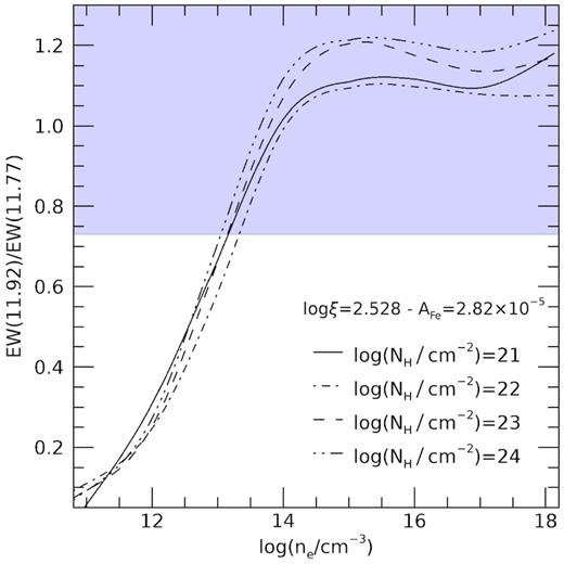
Ratio of equivalent widths of the absorption lines of the Fe xxii L doublet (EW(11.92)/EW(11.77Å)) as a function of the plasma density (n). The various lines indicate the relation between plasma density and line ratio for different column densities of the absorber. The violet area indicates the region consistent (at 1σ) with the observed line ratio.
By performing extensive cloudy simulations, we computed the doublet line ratio as a function of the plasma density for various values of the column density of the absorbing material (see solid, dashed and dot–dashed lines in Fig. 6). We confirmed that the ratio is a sensitive probe of the plasma density. In particular, the observed line ratio suggests a plasma density of n > 1013 cm−3. This result will be used in Section 9.3 to estimate the location of the ionized absorber.
6.2 Line shifts
The absorption line centroids in MXB 1659-298 are observed to shift with orbital phase, with a semi-amplitude of 90 km s−1 (Ponti et al. 2018). Such modulation is thought to trace the radial velocity curve of the primary. We note that the HETG observation analysed here covered two complete orbital periods. Therefore, we expect to see no systematic shift of the absorption lines, due to such orbital modulation (the main consequence being an artificial broadening of the lines). We also note that Sidoli et al. (2001) investigated the evolution of the Fe xxv and Fe xxvi line intensities as a function of orbital phase, finding no significant variation (despite intensity variations as large as a factor of 2 were not excluded).
The line centroids of all lines in the average spectrum are consistent with being at rest, with outflow or inflow velocities lower than 200 km s−1 (Table 2). In particular, we observed that the lines with the highest signal to noise indicated upper limits to any bulk flow velocity of less than 50–70 km s−1 (Table 2). Therefore, the observed ionized absorption is not due to a wind, it is instead associated with an ionized disc atmosphere.
6.3 The line-rich HETG spectrum fitted with self-consistent photo-ionization models
In this paragraph, we present the separate fit of only the Chandra HETG spectrum (0.8–7.3 keV; Table 3). In this way, the fit will be driven by the absorption lines only (e.g. without strong contamination from either the ionized Fe K edges, the broad Fe K line or the shape of the high-energy continuum).
Best-fitting parameters of the fit of the Chandra HETG spectra only. See the text for description of the various parameters. Symbols as in Table 1.
| OnlyChandraHETG soft state (2016-04-21) | |||||
|---|---|---|---|---|---|
| Model | C1 | C2 | C4 | C5 | |
| DBB + BB | xipcf(DBB + BB) | IA(DBB + BB) | IA∗IA(DBB + BB) | ||
| NH | ⋆ | 0.23 ± 0.01 | 0.22 ± 0.02 | 0.213 ± 0.008 | 0.192 ± 0.007 |
| Log (ξ1) | 4.26 ± 0.02 | |$3.85^{+0.04}_{-0.11}$| | >4.56 | ||
| Log |$(N_{\rm H_{1}})$| | ⋆ | 23.6 ± 0.1 | 23.6 ± 0.1 | 24.21 ± 0.02 | |
| Log (ξ2) | 3.33 ± 0.04 | ||||
| Log |$(N_{\rm H_{2}})$| | ⋆ | <22.5 | |||
| kTDBB | ♭ | 1.07 ± 0.10 | 1.2 ± 0.2 | 1.34 ± 0.07 | 1.34 ± 0.07 |
| NDBB | ‡ | 19 ± 6 | 12 ± 4 | |$9.9^{+2.4}_{-0.9}$| | |$9.9^{+1.8}_{-1.1}$| |
| kTBB | ♭ | 1.7 ± 0.2 | |$2.1^{+1.0}_{-0.3}$| | |$2.8^{+0.1}_{-0.5}$| | 2.8 ± 0.5 |
| NBB | ‡ | 5.0 ± 2.0 | 2.1 ± 1.5 | |$0.8^{+0.1}_{-0.4}$| | 0.83 ± 0.5 |
| cMEG | 1.03 ± 0.01 | 1.03 ± 0.01 | 1.03 ± 0.01 | 1.03 ± 0.01 | |
| Cstat/dof | 8299.5/6137 | 6750.3/6129 | 6543.0/6129 | 6514.2/6127 | |
As already evidenced from Section 5, we observed that the addition of an approximated ionized absorption component (model C2) to the disc blackbody and hot blackbody emission (C1) significantly improved the fit of the HETG spectrum of MXB 1659-298, during the soft state (ΔC − stat = 1549.2 for the addition of two new free parameters; see Table 3). Based on the observed soft state SED, we built a fully auto consistent photo-ionization model (IAsoft). The model table was computed through a cloudy computation, assuming constant electron density (ne = 1014 cm−3), turbulent velocity vturb = 500 km s−1 and Solar abundances.
We then substituted the approximated photo-ionized component with this self-consistent ionized absorber (C4). By comparing model C4 with C2, we observed a significant improvement of the fit (ΔC − stat = 207.3) for the same degrees of freedom (Table 3). This confirms that the array of absorption lines is better described by the self-consistent photo-ionization model, producing an acceptable description of the data. The ionized plasma is best described by a relatively large column density (log (NH/cm−2) = 23.6 ± 0.1) of highly ionized (|$\log (\xi /\mathrm{erg~cm~s}^{-1})=3.85^{+0.04}_{-0.11}$|) material. We note that these values are in line with what measured from XMM–Newton observations of MXB 1659-298 during the previous outburst (Sidoli et al. 2001; Díaz Trigo et al. 2006).
We then tested whether the ionized absorber is composed of multiple and separate components with, for example, different ionization parameters. We performed this by adding a second ionized absorber layer to the fit. We observed a slight improvement of the fit (ΔC − stat = 29.0 for the addition of 2 free parameters; Table 3). The two components of the ionized absorbers were split into a very high column density and ionization parameter component (log (NH/cm−2) ∼ 24.2 and log (ξ/erg cm s−1) > 4.5) and a much lower column density and ionization one (log (NH/cm−2) < 22.5 and log (ξ/erg cm s−1) ∼ 3.3), leaving the best-fitting parameters of the continuum emission consistent with the previous fit (Table 3).
Since the fit with two ionized absorption layers provided only a marginal improvement of the fit from a statistical point of view, we concluded that a single ionized absorption layer provided a good description of the absorption lines.
6.4 Stability curve
The red line in Fig. 7 shows the thermal equilibrium conditions of the absorber, once the ionized plasma is illuminated by the soft state SED (Fig. 3). The thermal equilibrium is the result of the competition between heating and cooling and the corresponding stability curve is inferred through extensive cloudy computations in the same way as described in Bianchi et al. (2017).
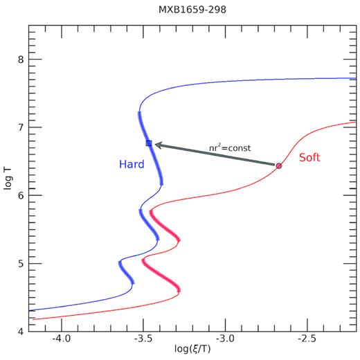
Photoionization stability curves of the ionized absorbing plasma when illuminated with the soft (red) and hard (blue) SEDs. The thick segments indicate the thermally unstable branches of the curves. The red circle indicates the position of the ionized absorber during the soft state. The absorber is thermally stable. The blue square indicates the expected condition of the absorber when illuminated by the hard state SED. Such conditions are thermally unstable.
As expected, we observed that the ionized absorber (i.e. disc atmosphere) is in thermal equilibrium during the soft state (see red point in Fig. 3). Actually, any equilibrium solution with plasma temperatures higher than kT ∼ 55 eV or lower than 3.4 eV would be stable, with only two small instabilities present between these two ranges.
7 BROAD-BAND FIT OF THE SOFT STATE SPECTRA
We started the broad-band fit of the soft state spectra of MXB 1659-298, by substituting the approximated photo-ionized absorber model (zxipcf) employed in model B3 (Section 5), with the fully auto consistent photo-ionized absorber model (B6; tbabs∗IAsoft(diskbb+bbody + nthcomp)) described in Section 6.3. We observed a significant improvement of the fit (ΔC − stat = −184.3 for the same dof), in agreement with the fact that the IAsoft model provides a superior description of the Chandra HETG spectra and the absorption lines. However, we noted that the best-fitting column density (log (NH/cm−2) = 24.25 ± 0.02 instead of 23.6 ± 0.2) and ionization parameter (log (ξ/erg cm s−1) = 4.54 ± 0.01 instead of |$3.85^{+0.04}_{-011}$|) of the ionized absorber were significantly larger than the best fit of the HETG data only. This variation was induced by the attempt of the model to reproduce the large residuals at 6–8 keV (see Fig. 2). The resulting best fit was therefore driven to an increased column density and ionization parameter of the absorbing plasma (compared with what was required by the absorption lines) in an attempt to enhance the depth of the ionized Fe K edges (|$E_{\rm Fe\, {\rm{\small XXV}}}=8.83$| and |$E_{\rm Fe\, {\small XXVI}}=9.28$| keV).
We noted that the remaining significant residuals in the 6–12 keV band were resembling a broadened Fe K α emission line (Fig. 2). We, therefore, added to the model a disc line component (B7; tbabs∗IAsoft(diskline+diskbb+bbody + nthcomp)). We assumed the line energy to be E = 6.4 keV (although the material in the inner accretion disc might be ionized), a disc inclination of 75° (Ponti et al. 2018), inner and outer radii of rin = 6 rg and rout = 1000 rg (where rg = GMNS/c2 is the gravitational radius, G is the Gravitational constant, MNS the NS mass, and c is the light speed). The free parameters of the model were the disc emissivity index αd and the line normalization. This provided a significant improvement, resulting in an acceptable fit (C − stat = 7584.7 for 7088 dof). The best-fitting line emissivity index and equivalent widths αd ∼ −2.6 and EW ∼ 250 eV are consistent with the expected values from a standard irradiated accretion disc (George & Fabian 1991; Matt, Perola & Piro 1991).
The addition of the disc-line component to the model allowed a better fit of the Fe K band, decreasing the depth of the ionized Fe K edges, therefore leading to best-fitting ionization parameter and column density of the ionized absorber consistent with the fit of the HETG data alone (log (NH/cm−2) ∼ 23.5 cm−2 and log (ξ/erg cm s−1) ∼ 3.8).
The observed and un-obscured 0.1–100 keV flux are F0.1–100 = 9.8 × 10⁻¹⁰ and 11.2 × 10⁻¹⁰ erg cm−2 s−1, respectively. The disc blackbody, blackbody, and Comptonization components carry 50 per cent, 17 per cent, and 30 per cent of the un-obscured 0.1–100 keV flux. The best-fitting continuum is described by a disc blackbody component with temperature of kTDBB ∼ 1.3 keV with an associated inner radius of rDBB ∼ 10 km, therefore comparable with the NS radius. The best-fitting blackbody emission kTBB ∼ 2.5 keV is hotter than the one of the accretion disc and is produced from a small region with a surface area of rBB ∼ 1.5 km2, likely associated with the boundary layer. At high energy (E ≥ 20 − 30 keV) a small contribution due to thermal Comptonization appears significant. Assuming an asymptotic photon index of Γ = 2, the best-fitting temperature of the Comptonising electrons is kTe ∼ 4 keV. This value is significantly lower than what is typically observed during the hard state or in BH systems. This is possibly induced by the cooling power of the abundant soft photons produced by the disc and/or boundary layer (Done & Gierliński 2003; Burke, Gilfanov & Sunyaev 2018).
8 HARD STATE OBSERVATIONS
To investigate the evolution of the disc atmosphere as a function of the accretion disc state and its response to the variation of the SED, we analysed the XMM–Newton observation that caught MXB 1659-298 in the hard state. The NuSTAR hard state observation (taken two days after) will be presented in a Degenaar et al. (in preparation).
Fig. 8 shows the light curve of the hard state XMM–Newton EPIC-pn observation. One bright burst (dark grey peak), two eclipses (lasting 930 s) as well as intense dipping activity are observed and removed. The black data in Fig. 9 show a clear drop, in the spectrum, at energies below 1 keV, suggesting the presence of neutral absorbing material. We fitted the persistent spectrum with an absorbed power-law spectrum (tbabs∗powerlaw in xspec). Although this model can reasonably reproduce the bulk of the observed X-ray emission (NH = 2.42 ± 0.02 × 1021 cm−2, ΓPL = 1.82 ± 0.05), large residuals make the fit unacceptable (χ2 = 2351.8 for 1782 dof; Table 4).
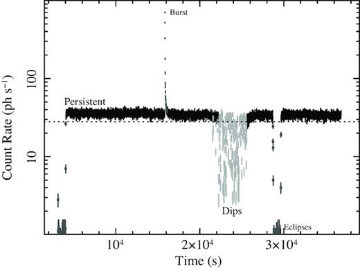
0.5–10 keV XMM–Newton light curve of MXB 1659-298 performed on 2015 September 26. The EPIC-pn exposure starts just before the eclipsed period (shown with dark grey squares). During the observation a clear burst is observed (shown with dark grey colours) as well as intense dipping activity (light grey colours). The black points show the persistent emission. The dotted line indicates the lower bound we use to identify persistent flux, with intervals dipping below this being selected as dips. Time bis of 10 s are used.
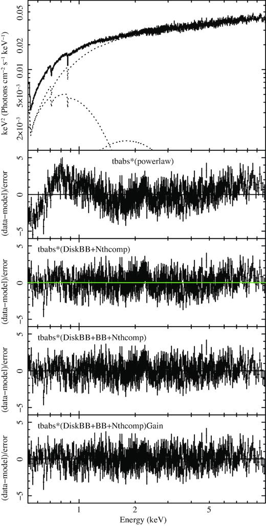
(Top panel) XMM–Newton EPIC-pn hard state spectrum fitted by the best-fitting model (disc blackbody plus blackbody and a dominant Comptonization components absorbed by neutral material). No signs of ionized absorption is present. (Centre top panel) Residuals once the data are fitted with an absorbed power law. (Centre panel) Residuals after fitting with an absorbed disc blackbody plus Comptonization model. (Centre bottom panel) Residuals after the addition of a blackbody component. (Bottom panel) Residuals after the consideration of a gain offset in the response files.
Best-fitting parameters of the XMM–Newton EPIC-pn hard state spectrum. A variety of spectral components, described in the text, are employed. Model H1 (tbabs(powerlaw)) is composed by a powerlaw absorbed by neutral material (tbabs). Model H2 (tbabs(diskbb + nthcomp)) considers the emission from a disc blackbody plus a thermal Comptonization component. Model H3 additionally considers the emission from a blackbody component (bbody: tbabs(diskbb+bbody + nthcomp)). Model H3gain applies a fit to the offset of the gain (with fixed slope) of the response matrices (gain ∗ tbabs(nthcomp+diskbb + bbody)). The following symbols mean: † Fixed parameter; ∣ In eV units; ⋄ Units of 10−2. Other symbols as in Table 1. Error bars indicate 90 per cent confidence, unless stated otherwise.
| Hard state -XMM–Newton | |||||
|---|---|---|---|---|---|
| Model | H1 | H2 | H3 | H3gain | |
| NH | ⋆ | 0.242 ± 0.02 | 0.31 ± 0.01 | 0.33 ± 0.02 | 0.33 ± 0.01 |
| Γ | 1.82 ± 0.05 | 1.810 ± 0.004 | 1.76 ± 0.02 | 1.74 ± 0.02 | |
| NPL | ⋄ | 2.66 ± 0.02 | |||
| kTe | ♭ | 17† | 17† | 17† | |
| Nnth | ⋄ | 2.58 ± 0.04 | 2.4 ± 0.1 | 2.4 ± 0.1 | |
| kTDBB | ♭ | 0.18 ± 0.01 | 0.18 ± 0.01 | 0.17 ± 0.01 | |
| NDBB | ‡ | 1900 ± 600 | 2400 ± 1200 | 3600 ± 1200 | |
| kTBB | ♭ | 0.45 ± 0.05 | 0.42 ± 0.07 | ||
| NBB | ‡ | 9 ± 5 | |$10^{+10}_{-4}$| | ||
| Gainoff | ∣ | 12 ± 3 | |||
| χ2/dof | 2351.8/1782 | 1844.5/1780 | 1820.9/1778 | 1784.8/1777 | |
Therefore, we added a disc blackbody component (diskbb) and substituted the power-law emission with a Comptonization component (nthcomp) absorbed by neutral material. We assumed a temperature of kTe = 17 keV for the Comptonising electrons. This temperature corresponds to the best-fitting value of the fit of the NuSTAR data, accumulated 2 d after the XMM–Newton observation (see Degenaar et al. in preparation). This model well reproduced the data (χ2 = 1844.5 for 1780 dof). The spectrum was dominated by the Comptonization component with Γ ∼ 1.8 and a cold (kTDBB = 0.19 ± 0.01 keV) disc blackbody component, with a large inner disc radius (rDBB ∼ 150 − 200 km) required by the data.
The further addition of a blackbody emission component slightly improved the fit (χ2 = 1820.9 for 1778 dof, with associated F-test probability 1 × 10⁻⁵). The best-fitting blackbody component was hotter (kTBB = 0.45 ± 0.05 keV) than the disc blackbody one (however colder than what is typically observed during the soft state) and produced by a small area with a radius of 9 km.
We noted a significant excess occurring at 2.2 keV, where the effective area experiences a drop due to the Au M edge. To determine the nature of such excess, we modified3 the gain in the response files until reaching the best fit. We observed a significant improvement of the fit (Δχ2 = 36.1 for 1 dof) with a gain offset of gainoff = 12 ± 3 eV. Such offset is smaller than the uncertainty on the calibration of the EPIC energy scale (see XMM-SOC-CAL-TN-0018). This suggested that such residual is instrumental and it will not be discussed further.4
Based on this best-fitting hard state model and the constraints from Swift-UVOT and NuSTAR (see Degenaar et al. in preparation) data, we reconstructed the ‘bona-fide’ hard state SED (black line, Fig. 3). The observed and un-obscured 0.1–100 keV flux are F0.1–100 = 2.9 × 10⁻¹⁰ and 3.9 × 10⁻¹⁰ erg cm−2 s−1, respectively. The disc blackbody, blackbody, and Comptonization components carry 15 per cent, 1 per cent, and 84 per cent of the un-obscured 0.1–100 keV flux.
No absorption line due to ionized iron appeared in the data. Indeed, we added a narrow (σ = 1 eV) absorption line with a Gaussian profile at the energy of the Fe xxv and Fe xxvi transitions and we obtained upper limits to their equivalent width of |${\rm EW_{Fe\, {\small XXV}}}\gt -10$| eV and |${\rm EW_{Fe\, {\small XXVI}}}\gt -13$| eV, respectively. The addition of a discline with the same profile as observed during the soft state (αd = −2.6) did not improve the fit, with an upper limit on the line equivalent width of EW < 80 eV.
No ionized emission or absorption line are detected in the RGS spectra, with upper limits of 4–8 eV on the Ly α transitions of the most abundant elements. We note, however, that such upper limits do not exclude that soft X-ray lines as observed during the soft state are present in the hard state.
9 DISCUSSION
We studied the evolution of the X-ray emission of MXB 1659-298, throughout the states, during its most recent outburst, We observed that a three-component continuum model (disc blackbody and Comptonization in addition to thermal emission from, e.g. the boundary layer) provided an adequate description of the data in both spectral states. The observed trends of the best-fitting parameters (i.e. lower disc temperatures, larger disc inner radii, and larger Comptonization fractions in the hard state) are in line with what is typically observed in accreting BH and-or other atoll sources (Lin et al. 2007; Dunn et al. 2010; Muñoz-Darias et al. 2014; Armas-Padilla et al. 2018).
The normalization of the disc blackbody component suggests that the accretion disc extends to radii comparable to the NS radius during the soft state, while it might be truncated during the hard state. In line with this, we observed broad residuals in the Fe K band, in the soft state. Such residuals are well reproduced by a relativistic disc line model with a standard line equivalent width (EW ∼ 250 eV), with a disc emissivity αd ∼ −2.6, off an highly inclined accretion disc (i = 75°) extending to few gravitational radii. Such broad feature appears less prominent during the XMM–Newton and NuSTAR hard state observations.
The persistent source emission is absorbed by a moderate column density of lowly ionized material that appears to vary from the soft (NH ∼ 0.21 ± 0.01 × 1022 cm−2) to the hard state (NH ∼ 0.33 ± 0.01 × 1022 cm−2). The observed variation is of the same order of magnitude of the one observed by Cackett et al. (2013) (i.e. from NH ∼ 0.2 ± 0.01 × 1022 cm−2 to NH ∼ 0.47 ± 0.13 × 1022 cm−2) during quiescence. Despite the origin of such variation is uncertain, it is clear than during outbursts dipping X-ray binaries can display variations of the column density of neutral absorption, by orders of magnitude (White & Mason 1985; Frank et al. 1987; Ponti et al. 2016). Therefore, despite we analysed only the persistent emission, the observed variation (of 40 per cent) is not surprising. Indeed, the observed fast variation suggests that at least the variable part of the column density of absorbing material is local to the source. If so, such material can potentially change its physical conditions (e.g. ionization, location), producing the observed variation. Additionally, we note that part of such difference could be driven by the distorting effects of dust scattering (e.g. induced by combination of the energy dependence of the dust scattering cross-section and the different spectral extraction regions; Trümper & Schönfelder 1973; Predehl & Schmitt 1995; Jin et al. 2017, 2018). Therefore, we caution the reader from deriving conclusions from this difference.5
9.1 Ionized absorber–state connection
MXB 1659-298 shows clear evidence for highly ionized (Fe K) absorption during the soft state that disappears (at least the Fe xxv and Fe xxvi lines) during the hard state. This similar behaviour is shared also by two of the best monitored atoll sources (Ponti et al. 2014, 2015, 2017) and it is ubiquitous in accreting BH binaries (Ponti et al. 2012).6 We note that, in BH systems, the observed wind–state connection has been occasionally ascribed to a variation of the geometry of the wind, or a variation of the magnetic field configuration, or a variation of the launching mechanism, etc. (Ueda et al. 2010; Miller et al. 2012; Neilsen & Homan 2012).
9.2 Stability of the disc atmosphere
As discussed in Section 6.4, the best-fitting ionized absorber parameters (log (ξ/erg cm s−1) = 3.76; log (NH/cm−2) = 23.48) correspond to a thermally stable solution during the soft state (Fig. 7). Given the properties of the disc atmosphere observed during the soft state, we can predict its behaviour during the hard state, under the reasonable assumption that the variations of the absorber are solely due to the different illuminating SED. Indeed, as a consequence of the variation of the SED, the ionization parameter is expected to vary following ξ = L/(nR2), if the density (n) and location (R) of the absorber remain unchanged (or that they both vary keeping nR2 constant). Indeed, in such a situation, the ionization parameter of the atmosphere would change in response to the variations of the source luminosity (L) following the relation: ξ = L/(nR2). Hence, we can estimate the expected ionization parameter during the hard state as: ξh = (ξsLh)/Ls (where Ls, Lh, ξs, and ξh are the soft and hard luminosities in the 0.1–100 keV energy band and ionization parameters, respectively), corresponding to log (ξh) ∼ 3.30 (see Fig. 7). Therefore, during the hard state the ionization parameter is lower than during the soft state. Indeed, despite the shape of the SED is harder, the lower hard state total luminosity implies lower ionization. Clearly, the hard state spectrum rules out the presence of an absorber with log (ξh/erg cm s−1) = 3.30 and log (NH/cm−2) = 23.48. This implies that the ionized absorber must have changed (i.e. nR2 or both) as a result of the variation of the SED. Indeed, we note that the estimated hard state parameters of the ionized absorbers fall on to an unstable branch of the thermal photo-ionization stability curve (Fig. 7). Therefore, most likely the absorber will migrate away from such unstable equilibrium, possibly towards a stable higher and/or lower ionization parameter (see Bianchi et al. 2017 for more details). We note that such behaviour is common to the classical hard (and hard-intermediate) state SED of BH LMXB. Therefore, this mechanism could be responsible for the observed ionized absorber–state connection.
9.3 Distance to the ionized absorber
The constraints on the ionized absorber density obtained in Section 6.1 from the Fe xxii doublet ratio can be used to estimate its distance from the irradiating X-ray source (R). Indeed, using the equation: R2 = L/nξ, we derived R < 1.5 × 1010 cm, for a source luminosity L ∼ 1.3 × 1037 erg s−1 and plasma ionization parameter log (ξ/erg cm s−1) ∼ 3.76, as observed during the soft state. Such distance corresponds to R ≤ 7 × 10⁴ rg and it is a significant fraction of the accretion disc size.
Assuming the outer disc radius (RD) to be 80 per cent of the primary’s Roche lobe radius (RL1), calculated by the approximate formula: RD = 0.8a × (0.46q−2/3)/[0.6q−2/3 + log(1 + q−1/3)], where q is the mass ratio m2/m1 between the masses of the primary and companion star in Solar masses ( Eggleton 1983) and a is the binary separation which can be conveniently expressed in the form: |$a=3.5\times 10^{10} (1+q)^{1/3} m_1^{1/3} P_{\rm orb}^{2/3}$| cm, where Porb is the orbital period in days (King et al. 1996), we computed the outer disc radius (for Porb = 7.11611 h, m1 = 1.4 and m2 = 0.6 M⊙; Ponti et al. 2018) to be RD = 6.2 × 1010 cm or 3.0 × 10⁵ rg. Therefore, the ionized plasma sits well inside the disc.
We also note that the plasma is located inside the Compton radius too. To estimate the latter, we first computed the Compton temperature (TC) by integrating the observed soft state SED and obtaining: TC = 1.57 × 10⁷ K. We then derived the Compton radius (RC) and the critical luminosity (Lcr) from the formulae: RC = (1018 × m1)/TC cm and |$L_{\rm cr}=0.03 L_{\rm Edd} / \sqrt{T_{\rm C}/10^8}$|, where LEdd is the Eddington luminosity (Begelman et al. 1983). The Compton radius resulted to be RC = 8.9 × 1010 cm and Lcr = 1.5 × 1037 erg s−1. We note that both the ionized plasma sits well inside the Compton radius (R < 0.17 × RC) and the soft state luminosity (L ∼ 0.87 × Lcr) is comparable if not smaller than the critical luminosity, therefore hampering the generation of a thermally driven wind. For these reasons, no thermal wind can be generated in MXB 1659-2987 and the absorber can be at rest, forming an accretion disc atmosphere.
9.4 Single or multilayer absorber and other approximations
The best-fitting model suggests that a single layer absorber with high column density and ionization parameter can reproduce the bulk of the absorption features in the average spectrum. At first, this appears rather surprising. Indeed, the large array of different transitions with significantly different ionization potential might carry information of a radial stratification of the ionization of the absorber, or be the consequence of significant variations over time of the plasma parameters. However, before properly addressing these very interesting scenarios, a detailed understanding of secondary effects impacting the expected results need to be fully carried out. Indeed, several of the strongest absorption lines are saturated (Ponti et al. in preparation), the ionized absorber is likely variable, the line broadening might be different from the value assumed in this work (vturb = 500 km s−1). We therefore leave such questions for future investigations.
10 CONCLUSIONS
We studied the evolution of the X-ray emission of the accreting NS LMXB MXB 1659-298, comparing the soft and hard accretion states. During the soft state, we detected 60 absorption lines (of which 21 at more than 3σ), that is about one order of magnitude more lines compared to previous works (six lines were detected by Sidoli et al. 2001; Díaz Trigo et al. 2006). This allows us to place tighter constraints on the physical properties of the absorbing plasma (log (ξ/erg cm s−1) ∼ 3.8, log (NH/cm−2) ∼ 23.5), to demonstrate that both the low-energy transitions and Fe K lines are at rest, without the requirement to invoke a mildly outflowing disc atmosphere. The repeated detection of a high-ionization absorber during the soft states in two different outbursts (Sidoli et al. 2001; Díaz Trigo et al. 2006; this work) suggests the persistent presence of such component during the soft state. The new data show that the high-ionization absorption (traced by the Fe xxv and Fe xxvi lines) significantly weakens/disappears during the hard state, indicating a physical change of the absorber (disc atmosphere) between the two states. This is likely a consequence of a photo-ionization thermal instability that drives the Fe K absorber to new equilibria consistent with fully or lowly ionized plasma (Bianchi et al. 2017). Thanks to the tentative detection of one of the lines of the Fe xxii doublet, we also constrained the density of the absorber (ne > 1013 cm−3).
Comparison with similar works
While this work was refereed, a similar paper has been accepted (Sharma et al. 2018) and another has been submitted and posted on arXiv (Iaria et al. 2018). Sharma et al. (2018) finds very similar results to the ones presented here. Different components are, instead, investigated by Iaria et al. However, we refrain from performing a detailed comparison, because that work is still in the refereeing process.
ACKNOWLEDGEMENTS
The authors wish to thank Norbert Schartel and Fiona Harrison for approving the XMM–Newton and NuSTAR DDT observations of MXB 1659-298. GP acknowledges financial support from the Bundesministerium für Wirtschaft und Technologie/Deutsches Zentrum für Luft- und Raumfahrt (BMWI/DLR, FKZ 50 OR 1812, FKZ 50 OR 1715 and FKZ 50 OR 1604) and the Max Planck Society. SB acknowledges financial support from the Italian Space Agency under grants ASI-INAF I/037/12/0 and 2017-14-H.O. BDM acknowledges support from the Polish National Science Center grant Polonez 2016/21/P/ST9/04025 and from the European Union’s Horizon 2020 research and innovation programme under the Marie Sklodowska-Curie grant agreement No 798726. ND is supported by a Vidi grant from the Netherlands Organization for Scientific research (NWO).
Footnotes
The Chandra HETG frame time does not allow to constrain the spectral state through timing.
We also tried fixing the energy of this transition to that expected if the line experienced the same shift as the λ = 11.920 line (Section 6.2), which did not change our result.
We performed this by employing the gain model to the response files. The gain command shifts the energies on which the response matrix is defined as well as the effective area in such a way that Enew = E/sl − gainoff (where E and Enew are the original and shifted energies). We searched for the best-fitting offset in the gain, however we kept the slope fixed to the default value (sl = 1).
Please note that we did not use the gain model any further in this work.
In theory, by characterizing the shape and the variability of the dust scattering halo, it is possible to correct the spectrum of the source, therefore to verify the reality of the column density variation (see for example the case of AX J1745.6-2901; Jin et al. 2017, 2018). Despite we recently developed such spectral corrections for various extracting regions of modern X-ray telescopes, unfortunately these are not applicable to first-order grating data, because of the complexity of the source extraction in dispersed spectra; Jin et al. 2017, 2018).
Exceptions to this trend have been reported during the hard state outburst of V404 Cyg (King et al. 2015) and in some Z-sources (Homan et al. 2016). The latter class of sources are characterised by more complex behaviours and state classification as well as larger luminosities, compared to atoll NS.
Although this does not apply to magnetic winds.
